www.ocean-sci.net/8/885/2012/ doi:10.5194/os-8-885-2012
© Author(s) 2012. CC Attribution 3.0 License.
Ocean Science
Towards high resolution mapping of 3-D mesoscale dynamics from
observations
B. Buongiorno Nardelli1,2, S. Guinehut3, A. Pascual4, Y. Drillet5, S. Ruiz4, and S. Mulet3
1Istituto di Scienze dell’Atmosfera e del Clima, Roma, Italy 2Istituto per l’Ambiente Marino Costiero, Napoli, Italy
3CLS-Space Oceanography Division, Ramonville Saint-Agne, France 4IMEDEA(CSIC-UIB), Esporles, Spain
5Mercator Oc´ean, Ramonville Saint-Agne, France
Correspondence to:B. Buongiorno Nardelli ([email protected]) Received: 1 March 2012 – Published in Ocean Sci. Discuss.: 14 March 2012
Revised: 31 July 2012 – Accepted: 19 September 2012 – Published: 19 October 2012
Abstract. The MyOcean R&D project MESCLA
(MEsoSCaLe dynamical Analysis through combined model, satellite and in situ data) was devoted to the high resolution 3-D retrieval of tracer and velocity fields in the oceans, based on the combination of in situ and satellite observations and quasi-geostrophic dynamical models. The retrieval techniques were also tested and compared with the output of a primitive equation model, with particular attention to the accuracy of the vertical velocity field as estimated through the Qvector formulation of the omega equation. The project focused on a test case, covering the region where the Gulf Stream separates from the US East Coast. This work demonstrated that innovative methods for the high resolution mapping of 3-D mesoscale dynamics from observations can be used to build the next generations of operational observation-based products.
1 Introduction
Ocean science and operational oceanography are based on the analysis of the space and time distribution of the pa-rameters that characterize the state of the sea under obser-vation. In principle, these state variables could be estimated directly from measurements, at least for the physical compo-nent of the system, usually including velocity, pressure, tem-perature and salinity (density). The system evolution could then be forecasted through the fundamental laws of oceanic physics, provided the external forcings are also known
(un-less a fully coupled ocean–atmosphere model is considered, in which case the state variables include part of the forcings). In practice, the determination of the distribution of the ocean state variables is restrained by sampling, instrumental and re-source limitations, and their forecasting is complicated by the non-linear nature of the equations that drive the system, gen-erally requiring numerical solution, and by the huge number of degrees of freedom involved in corresponding models. All these elements make the combination and analysis of the few available observations a challenge for physical oceanogra-phers, especially if the phenomena of interest are ubiquitous in the global oceans and involve relatively small space and time scales, such as mesoscale processes.
Conversely, a purely observation-based approach, aiming to retrieve the three-dimensional (3-D) mesoscale dynam-ics from a statistical and/or empirical combination of in situ and satellite observations, has received limited recognition until now. This is partly related to the limits of present observation-based products, namely to their relatively low resolution, and to the difficulties in providing any indirect estimate of the ocean currents going beyond the simple geostrophic velocities (e.g. as usually obtained from satel-lite altimetry or dynamic heights). Moreover, especially for model validation purposes, there is a general tendency to look at each measured parameter separately (i.e. through univariate approaches), instead of considering the combina-tions of available observacombina-tions as incomplete realizacombina-tions of the system state. Conversely, our experience of the way the oceans behave indicates that the effective degrees of freedom in the system are significantly less than the number of vari-ables involved (i.e. covariance/autocorrelation reduces the effective number of independent data), so that multivariate reduced-space analyses can provide a more efficient descrip-tion of the system state than univariate approaches.
In fact, even if different multivariate techniques have been proposed until now to retrieve 3-D fields of temperature and salinity from combined observations, only a few of these have been translated into operational products (e.g. Fox et al., 2002; Guinehut et al., 2004). One of these products, named ARMOR3D, has been included in the GMES My-Ocean project catalogue as a “core” product (see also Guine-hut et al., 2012), but its spatial resolution can be presently classified only as “eddy permitting”, not exceeding 1 / 3◦.
The development of higher resolution observation-based 3-D fields might thus contribute to a more efficient analysis of observations and model validation through more advanced comparisons than those based on climatologic fields or sparse observations of temperature, salinity or velocities.
In this context, the MyOcean project (through its first open call for research and development) funded a small re-search initiative (MESCLA – MEsoSCaLe dynamical Analy-sis through combined model, satellite and in situ data, 2010– 2012) devoted to the high resolution 3-D retrieval and anal-ysis of tracer fields, horizontal and vertical velocities in the oceans based on the combination of in situ and satellite ob-servations and simplified diagnostic models, and on their comparison with primitive equation model output. MESCLA rationale lies in the fundamental role played by the mesoscale in modulating the ocean circulation and the fluxes of heat, freshwater and biogeochemical tracers between the surface and the deeper layers.
In fact, in order to correctly retrieve the vertical veloci-ties associated with mesoscale features, one should be able to resolve very small scales, i.e. down to less than 10 km (for a complete review on the topic, see Klein and Lapeyre, 2009). As said, present 3-D observation-based systems are far enough from being able to correctly reproduce the global variability at these scales (Willis et al., 2003; Roemmich
and Gilson, 2009; Von Schuckmann et al., 2009; Guinehut et al., 2004, 2012; Larnicol et al., 2006). Moreover, while the vertical component of ocean currents can be diagnosed in primitive equation numerical models by solving the conti-nuity equation, the same technique is not applicable to direct observations. This is due, on one hand, to the few current measurements available, and, on the other hand, to the high error that would result from the computation of the diver-gence from measured horizontal velocities, which may in-clude significant instrumental errors. It is also clearly impos-sible to use the continuity equation to estimate the vertical velocities from dynamic heights (computed from tempera-ture and salinity profiles), as the geostrophic velocities are non-divergent by definition. On the other hand, simplified di-agnostic models can be applied to retrieve the vertical veloc-ity field from both 2-D and/or 3-D estimates of geostrophic currents and density fields (e.g. Tintor´e et al., 1991; Allen and Smeed, 1996; Buongiorno Nardelli et al., 2001; Pascual et al., 2004; Klein et al., 2009; Isern-Fontanet et al., 2008; Ruiz et al., 2009).
In this framework, the first step in our work consisted of improving the existing MyOcean observation-based products (ARMOR3D, Guinehut et al., 2012) and in the development and testing of new high resolution horizontal interpolation and vertical extrapolation techniques (Buongiorno Nardelli, 2012; Buongiorno Nardelli et al., 2006; Buongiorno Nardelli and Santoleri, 2004, 2005), analysing the scales they are ef-fectively resolving. As a second step, a quasi-geostrophic (QG) diagnostic numerical model (theQvector formulation of the omega equation) has been used to estimate the verti-cal velocities (Pascual et al., 2004; Ruiz et al., 2009). The omega equation was applied to different MyOcean products (both model and observation-based) in order to quantify the differences/limitations in the diagnostic tools used and the impact of the spatial resolution on the retrieved velocity. The results of these two steps are the subject of the present paper. It is worth noting that this work represents the first attempt to apply purely observation-based 3-D retrieval techniques at high resolution (also resolving mesoscale quasi-geostrophic dynamics) to obtain data that could be produced routinely within an operational system (namely from near real-time, freely available data, and potentially with global coverage). However, given the lack of independent (direct) measure-ments of the vertical velocities, a full validation of the new products is clearly not possible. Consequently, the approach followed here relies on the comparison between all the dif-ferent products, concentrating on a test case.
mesoscale activity associated with its flow on the vertical and cross-front exchanges (e.g. Bower, 1989; Bower and Rossby, 1989; Lindstrom et al., 1997; Joyce et al., 2009; Thomas and Joyce, 2010). It is also one of the few areas where direct mea-surements of the vertical exchanges associated with frontal meanders and mesoscale instabilities have been collected and analysed (Bower and Rossby, 1989).
Our test case focused on a specific day, 17 October 2007, when three large and well developed Gulf Stream meanders were observed between 65◦W and 50◦W. The core of the current is well identified by the comparison of the surface ab-solute dynamic topography (ADT) field with corresponding SST (sea surface temperature) and SSS (sea surface salin-ity) patterns, shown in Fig. 1. Upstream is a thin warm water tongue which develops into a steep meandering thermal and salinity front between 38◦N and 42◦N. The strongest
gradi-ents are observed at the first meander, around 62◦W/41◦N.
To summarize, after presenting the dataset used (Sects. 2 and 3), this paper will focus on:
– the strategies adopted to increase the effective res-olution of the observation-based products (Sect. 4), namely:
– the integration of different high resolution Sea Surface Temperature level 4 products (SST L4, i.e. interpolated data) in the ARMOR3D processing (Sect. 4.1);
– the integration of the new high resolution Sea Surface Salinity (SSS L4) product (Buongiorno Nardelli, 2012) in the ARMOR3D processing (Sect. 4.1);
– the implementation of additional extrapolation method-ologies to obtain high resolution 3-D re-analyses based on the high resolution Sea Surface Salinity product, on one selected high resolution SST L4 product and stan-dard altimeter products (Sect. 4.2);
– the comparison of the various 3-D reconstructed fields, mainly focusing on the spatial scales that they are effec-tively able to resolve (Sect. 4.3);
– the diagnostic model used to retrieve the quasi-geostrophic vertical velocity field from the improved observation-based density and geostrophic velocity fields and its validation by comparison with the My-Ocean Mercator Oc´ean 1 / 4◦ and 1 / 12◦ resolution
model vertical velocities (Sects. 5.1 and 5.2);
– the impact of the effective product resolution on the estimation of the vertical velocity field from the 3-D observation-based products (Sect. 5.3) and an example of the dynamical interpretation of the vertical veloc-ity field concentrating on a specific mesoscale feature (frontal meander).
Fig. 1. (a)SST (ODYSSEA L4),(b)SSS (MESCLA HR) and(c)
SSH (AVISO) over the Gulf Stream area for the 17 October 2007.
2 Observations
In this study, two 3-DT /S retrieval techniques are consid-ered: ARMOR3D (Guinehut at al., 2012) and the multivari-ate EOF reconstruction (mEOF-r) (Buongiorno Nardelli and Santoleri, 2005). Both methods require, on one hand, a his-torical in situ dataset to estimate the correlations between the parameters of interest (namely, temperature, salinity and steric height) or to identify their main statistical or empirical modes of variability, and, on the other hand, surface measure-ments of at least some of these parameters to be able to ex-trapolate their vertical profiles. In the following, the datasets used for this work are briefly described.
2.1 In situ data
Coriolis/Argo for more recent data (http://www.coriolis.eu. org), and from the EN3 dataset for the historical data (Ingleby and Huddleston, 2007; http://www.metoffice.gov.uk/hadobs/ en3/). Similarly, the dataset used to test the mEOF-r vertical extrapolation techniques consists of the quality controlledT
andSprofiles measured by Argo and CTD sensors and dis-tributed by the MyOcean In Situ Thematic Assembly Cen-tre (more precisely, these are the profiles used by Coriolis In Situ Analysis System (ISAS) to produce their global temper-ature and salinity 3-D fields). The same dataset served also to develop the MESCLA high resolution SSS product (Buon-giorno Nardelli, 2012). These observations are pre-processed according to Argo recommendations for data quality control (Wong et al., 2012).
2.2 Surface data
2.2.1 SSS
The Sea Surface Salinity L4 data used as input to the 3-D reconstructions (section 4) has been developed in the frame-work of the MESCLA project (Buongiorno Nardelli, 2012). Its space–time resolution is 1 / 10◦, daily. The method used to retrieve this high resolution SSS field is based on an optimal interpolation (OI) algorithm that interpolates in situ salin-ity observations including satellite high-pass filtered SST in the determination of the weights used to interpolate SSS ob-servations (using 1 / 10◦ODYSSEA SST L4 as input). SSS
is represented as a function of space, time and SST (it is thus defined in a four-dimensional space), and a “general-ized” distance is used to define a new covariance model that thus includes a thermal decorrelation term. In practice, this covariance function associates a higher weight to the SSS observations that lie on the isothermal of the interpolation point with respect to observations taken at the same temporal and spatial separation but characterized by different SST val-ues. As satellite SST coverage and resolution is significantly higher with respect to in situ SSS observations, this method improves the interpolated field resolution not just in terms of grid spacing, but also in terms of the space–time features that are effectively retrieved. The covariance function parameters (i.e. spatial, temporal and thermal decorrelation scales) and the noise to signal ratio have been determined empirically, as fully described in Buongiorno Nardelli (2012). Hereafter, this SSS product will be called MESCLA HR SSS.
2.2.2 SLA/ADT
The altimeter Sea Level Anomalies (SLA) and Abso-lute Dynamic Topography (ADT) gridded data used for the 3-D retrieval are those produced and disseminated by the SSALTO/DUACS centre and represent the MyOcean Sea Level Thematic Assembly Centre intermediate product (AVISO, 2012). They are obtained as daily combined maps from all processed altimeters (Jason-1, Jason-2 and Envisat
for the DT products used in our study) with a 1 / 3◦horizontal
resolution.
2.2.3 SST
Different satellite SST datasets have been used for the differ-ent phases of the work, each characterized by differdiffer-ent nom-inal and effective resolution (as summarized in Table 1 and discussed in Sect. 4.3). In fact, as discussed by Reynolds and Chelton (2010), the true resolution of a L4 product is given by a combination of the grid spacing and of the analysis pro-cedures and configurations applied (e.g. weighting functions and background fields). As a consequence, while combined ARMOR3D product is based on the Reynolds Optimally In-terpolated L4 SST, at 1 / 4◦, corresponding to MyOcean V1 product (Larnicol et al., 2006; Guinehut et al., 2012), the higher resolution tests on ARMOR3D system have been per-formed on the ODYSSEA L4 data produced by Ifremer in the framework of the MERSEA project and maintained as part of MyOcean (Autret and Pioll´e, 2007), and on the Operational SST and Sea Ice Analysis system (OSTIA, see Donlon et al., 2011) also distributed as part of the MyOcean Sea Surface Temperature Thematic Assembly Centre. ODYSSEA pro-vides daily SST estimates on a 1 / 10◦ grid for the Global Ocean, based on both infrared and microwave measurements, while OSTIA L4 is available on a 1 / 20◦horizontal grid and includes also in situ SST measurements.
3 Model data
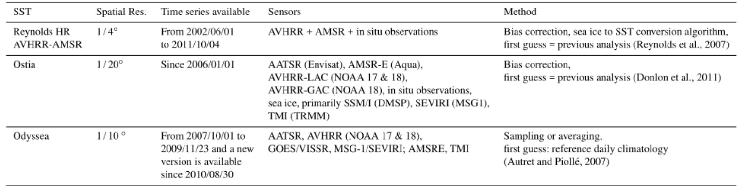
Table 1.Description of the L4 SST products used.
SST Spatial Res. Time series available Sensors Method
Reynolds HR 1 / 4◦ From 2002/06/01 AVHRR + AMSR + in situ observations Bias correction, sea ice to SST conversion algorithm,
AVHRR-AMSR to 2011/10/04 first guess = previous analysis (Reynolds et al., 2007)
Ostia 1 / 20◦ Since 2006/01/01 AATSR (Envisat), AMSR-E (Aqua), Bias correction,
AVHRR-LAC (NOAA 17 & 18), first guess = previous analysis (Donlon et al., 2011)
AVHRR-GAC (NOAA 18), in situ observations, sea ice, primarily SSM/I (DMSP), SEVIRI (MSG1), TMI (TRMM)
Odyssea 1 / 10◦ From 2007/10/01 to AATSR, AVHRR (NOAA 17 & 18), Sampling or averaging,
2009/11/23 and a new GOES/VISSR, MSG-1/SEVIRI; AMSRE, TMI first guess: reference daily climatology
version is available (Autret and Pioll´e, 2007)
since 2010/08/30
of instability of the water column. All these options are clas-sical and used in the global ocean model as mentioned in Barnier et al. (2006). The atmospheric forcing for the real time production is based on daily averages of the atmospheric variables or flux provided by the ECMWF real time forecast-ing system. The assimilation scheme (Tranchant et al., 2008) used in both configurations is based on the singular evolutive extended Kalman (SEEK) filter which allows assimilation of the sea level along-track satellite observations delivered by the MyOcean Sea Level Thematic Assembly Centre, the temperature and salinity profiles from the MyOcean In Situ Thematic Assembly Centre and the RTG (Real-Time-Global) sea surface temperature (http://polar.ncep.noaa.gov/sst/oper/ Welcome.html). The model outputs used in this study are based on the “best analysis”, which is performed every week with a one week delay in time to assimilate the most of ob-servations over a one week assimilation window. This sys-tem was the global forecasting syssys-tem operated during the V0 phase of MyOcean. The vertical velocity which is used as “reference” in this study to analyse the limits of the quasi-geostrophic omega equation is computed by an upward inte-gration of the horizontal divergence from the bottom (Madec, 2008) which is the standard way to compute the vertical ve-locities in the NEMO model in the case of a free surface con-dition.
4 3-D reconstruction
Several dynamic, variational, statistical and empirical tech-niques have been developed in the past to retrieve 3-D fields from a combination of in situ and satellite data (e.g. Carnes et al., 1994; Gavart and De Mey, 1997; Pascual and Gomis, 2003; Meinen and Watts, 2000; Watts et al., 2001; Mitchell et al., 2004). In fact, many of these methods are technically similar to some assimilation schemes (optimal interpolation-like), with the difference that the first guess used, i.e. the background analysis, is given by an average over the obser-vations instead of a numerical model forecast. The error as-sociated with this analysis thus represents the actual system variability. In essence, most statistical methods are based on
the analysis of covariance relative to a set of in situ data pro-files and on the identification of the principal modes charac-terizing the latter. However, the accuracy of each technique depends on the choice of the variables characterizing the state of the system, as well as on the number of degrees of free-dom absorbed by each method (e.g. Buongiorno Nardelli and Santoleri, 2004).
Univariate techniques such as single EOF (empirical or-thogonal function) reconstruction analyze the principal com-ponents of each parameter along the water column and hy-pothesize a relationship between the amplitude of such com-ponents and a (not necessarily linear) combination of sur-face parameters (Carnes et al., 1994). Simpler methods, as the one used within ARMOR3D, assume a direct correla-tion between surface and deep values (Guinehut et al., 2012). The new methods considered within MESCLA are based on multivariate approaches (multivariate EOF reconstruction, mEOF-r). These methods analyze the steric height, temper-ature and/or salinity covariance and reconstruct the vertical profiles via a combination of a limited number of modes. Fol-lowing an idea first proposed by Pascual and Gomis (2003), they include an approximation of the geopotential stream function (the steric height profile) in the status vector, thus more directly correlating physical–chemical parameter vari-ability to dynamics. The application of these methods already yielded promising results, also compared to empirical meth-ods such as the computation of the gravest empirical modes (Buongiorno Nardelli and Santoleri, 2005).
4.1 Increasing ARMOR3D spatial resolution
The MyOcean combined ARMOR3D product is computed every week (Wednesday fields) on a 1 / 3◦Mercator horizon-tal grid, which corresponds to the altimeter SLA grid and from the surface down to 1500 m depth on 24 vertical lev-els. ARMOR3D method, thoroughly described in Guinehut et al. (2012), improves a climatological first guess using two main steps. At first, synthetic temperature (T) profiles are estimated by extrapolating altimeter and SST data through a multiple linear regression method and covariances computed from historical data. For synthetic salinity (S) profiles, the method uses only altimeter data. The multiple/simple linear regression methods are expressed as:
T (x, y, z, t )=α(x, y, z, t )·SLA′(x, y, t )
+β(x, y, z, t )·SST′(x, y, t )+Tclim(x, y, z, t )
and
S(x, y, z, t )=γ (x, y, z, t )·SLA′(x, y, t )
+Sclim(x, y, z, t ),
where SLA′ and SST′ denote anomalies from the ARIVO
monthly climatology (Gaillard and Charraudeau, 2008),
TclimandSclimdenote the ARIVO monthly fields, andα,β andγ are the regression coefficients of the SLA and SST onto temperature and of SLA onto salinity, respectively. They vary with depth, time and geographical location and are ex-pressed as covariances between the variables (only thez vari-able is indicated here for clarity):
α(z)=
SST′,SST′·
SLA′, T′(z)−
SLA′,SST′·
SST′, T′(z)
SLA′,SLA′·
SST′,SST′−
SLA′,SST′2 ,
β(z)=
SLA′,SLA′·
SST′, T′(z)−
SLA′,SST′·
SLA′, T′(z)
SLA′,SLA′·
SST′,SST′−
SLA′,SST′2 ,
and
γ (z)=
S′(z),SLA′
SLA′,SLA′.
Successively, the synthetic profiles (hereafter referred to as synthetic ARMOR3Dfields) are combined with in situ tem-perature and salinity profiles using an optimal interpolation method (Bretherton et al., 1976) to create the combined AR-MOR3D product. The current paper focuses on the synthetic ARMOR3D fields.
As a preliminary step, ARMOR3D performs some crucial processing of altimeter data, being able to extract the steric contribution to the sea level variations consistent with the first 1500 m depth (filtering out the eustatic component and the deep steric contribution). This pre-processing is based on regression coefficients deduced from an altimeter/in situ comparison study (Guinehut et al., 2006; Dhomps et al., 2011).
In the present work, the three SST products described in Sect. 2.2.3 have been used to test the impact of SST reso-lution on the syntheticT field estimation (step one of the method). Additionally, the use of MESCLA HR SSS fields has also been tested for the reconstruction of the synthetic salinity. While the synthetic ARMOR3D salinity fields is ob-tained with a simple linear regression to altimeter SLA, the method has been thus modified to a multiple linear regression method (as for temperature) to include also the information from SSS. The salinity field is now calculated from the fol-lowing equation:
S(x, y, z, t )=λ(x, y, z, t )·SLA′(x, y, t )
+θ (x, y, z, t )·SSS′(x, y, t )+Sclim(x, y, z, t ),
with again the regression coefficients expressed as:
λ(z)=
SSS′,SSS′
·
SLA′, S′
(z)
−
SLA′,SSS′
·
SSS′, S′
(z)
SLA′,SLA′
·
SSS′,SSS′
−
SLA′,SSS′2 ,
and
θ (z)=
SLA′,SLA′·SSS′, S′(z)−SLA′,SSS′·SLA′, S′(z)
SLA′,SLA′
·
SSS′,SSS′
−
SLA′,SSS′2 .
All tests required us to interpolate the altimeter SLA onto each SST grid (i.e. interpolating the original data at 1 / 4◦, 1 / 10◦and 1 / 20◦, respectively). Actually, this interpolation has to be performed with particular care in order not to in-troduce a spurious signal. After having tested different meth-ods (simple bilinear interpolation, Akima spline), a classical spline method has been chosen.
4.2 mEOF-reconstruction
4.2.1 Method
The multivariate EOF reconstruction (mEOF-r) technique is based on the analysis salinity, temperature and steric height profiles through a multivariate EOF decomposition and on the availability of corresponding surface values (Buongiorno Nardelli and Santoleri, 2005).
Here, we will briefly recall how mEOF-r works. A sin-gle 3m×n multivariate observation matrix X is obtained from the three original sets of data, each of m×n dimen-sions, wherenis the number of measurements (stations) and
X=
T (0, r1) T (0, r2) . . . T (0, rn)
..
. ... . . . ...
T (zm, r1) T (zm, r2) . . . T (zm, rn)
S(0, r1) S(0, r2) . . . S(0, rn)
..
. ... . . . ...
S(zm, r1) S(zm, r2) . . . S(zm, rn)
SH(0, r1) SH(0, r2) . . . SH(0, rn)
..
. ... . . . ...
SH(zm, r1)SH(zm, r2) . . .SH(zm, rn)
To compute the multivariate EOF, the singular value decom-position of this new matrix of data is performed. In that way, “multi-coupled” modes are identified, each containing the three patterns corresponding to the parameters considered.
T (z, r),S(z, r)and SH(z, r)can thus be expanded in terms of
these three series of patterns. The same coefficient/amplitude (ak)is found for all parameters,Lk,Mk andNk being the
modes:
T (z, r)=
n
X
k=1
ak(r)Lk(z)
S(z, r)=
n
X
k=1
ak(r)Mk(z)
SH(z, r)=
n
X
k=1
ak(r)Nk(z).
If these expansions are limited to the first three modes, the vertical profiles can be estimated from the surface values (z=0) of the three parameters solving the system fora1,a2 anda3and substituting them in the truncated expansions:
a1(r)L1(0)+a2(r)L2(0)+a3(r)L3(0)=T (0, r)
a1(r)M1(0)+a2(r)M2(0)+a3(r)M3(0)=S(0, r)
a1(r)N1(0)+a2(r)N2(0)+a3(r)N3(0)=SH(0, r)
.
Of course, it is also possible to truncate the expansions to the second mode (or to the first one), which actually means that only two (one) surface parameters are sufficient to retrieve the whole profiles. Similarly, the whole analysis can be per-formed directly on two sets of parameters at a time.
The mEOF-r method requires a training dataset of T,
S and SH profiles to extract the main vertical modes of (co)variability. This training dataset might be selected dif-ferently at each grid point on the basis of different criteria: fixing a space and/or time search radius (e.g. 1000 km, week, month, or year), or keeping only the nearestnprofiles, etc. Depending on this choice, one may end up with different reconstruction models (i.e. different mEOFs) for each grid point or with a single set of modes. After some preliminary hindcast tests (not shown), it was decided to select all the profiles collected in the domain within a monthly window.
Given the sparse, even though regular, distribution of data in the trainingset, this was found to be the simplest but also most reliable way to estimate EOFs.
Similarly to the pre-processing performed by ARMOR3D, in order to retrieve the 3-D vertical fields from surface data, a preliminary step is to estimate/extract the surface steric heights from satellite altimeter data. Actually, there is no way to evaluate the deeper baroclinic and the barotropic contribu-tions from altimeter data and surface measurements alone. As a simple approximation, this estimation is reduced here to an adjustment of the ADT to minimize the differences between the steric height computed from simultaneous (or quasi-simultaneous) in situ profiles and co-located ADT es-timates (through a simple regression). In contrast to Guine-hut et al. (2012), who compute spatially varying climato-logical regression coefficients between co-located dynamic height anomaly computed from Argo T /S profiles and sea level anomaly (SLA) altimeter data, this adjustment has been performed here considering weekly matchups and a single regression. The adjusted ADT will be called in the follow-ing surface steric height (SSH). The in situT /Sprofiles de-scribed in Sect. 2.1 were re-interpolated at 10 dbar resolu-tion down to 1000 dbar, and steric height profiles were ob-tained taking 1000 dbar as reference pressure level. These data have been used as training dataset, while the same al-timeter ADT/SLA data, ODYSSEA SST L4 and MESCLA HR SSS L4 data used for the tests on ARMOR3D (Sect. 2.2) were used as surface input for the mEOF-r technique.
4.2.2 Hindcast evaluation of the mEOF-r performance in the Gulf Stream area
The hindcast validation was applied to the mEOF-r con-figurations listed below:
1. mEOF-r(T-S-SH): The mEOFs are computed from T,
Sand SH profiles, and corresponding synthetic profiles are obtained using SST, SSS and SSH as input data (the amplitude of the first 3 modes is retrieved).
2. mEOF-r(T-S-SH)SST-SSH: The mEOF are computed fromT,Sand SH profiles, and corresponding synthetic profiles are obtained using only SST and SSH as input data (the amplitude of the first 2 modes is retrieved). 3. mEOF-r(T-S-SH)SSS-SSH: The mEOF are computed
fromT,Sand SH profiles, and corresponding synthetic profiles are obtained using only SSS and SSH as input data (the amplitude of the first 2 modes is retrieved). 4. mEOF-r(T-SH): The mEOF are computed fromT and
SH profiles only, and corresponding synthetic profiles are obtained using SST and SSH as input data (the am-plitude of the first 2 modes is retrieved).
5. mEOF-r(S-SH): The mEOF are computed from S and SH profiles only, and corresponding synthetic profiles are obtained using SSS and SSH as input data (the am-plitude of the first 2 modes is retrieved).
Mean bias error (MBE) and standard deviation error (STDE) profiles for both temperature and salinity are shown in Fig. 2a and b, respectively. It is interesting to observe that the syn-thetic mEOF-r MBE is generally quite small. The mEOF-r provides the smallest STDE errors when only two modes are considered, both in the trivariate formulation and in the bi-variate one.
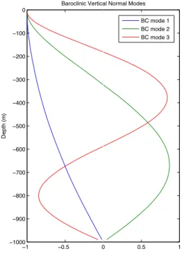
A simple explanation for this may be found looking at the mEOF modes (Fig. 3) and corresponding explained covari-ance percentage, and by comparing them with the dynami-cal modes that can be inferred from the mean stratification profileN2(Brunt–V¨ais¨al¨a frequency), as computed from the training dataset. In fact, the first mEOF mode explains an extremely high percentage of the variance (almost 99 %). If we look at the corresponding SH profile, it displays a quite smooth shape, increasing from zero at the reference level to a maximum at surface. This first mode closely reminds the first baroclinic mode that can be estimated from the linearized quasi-geostrophic vorticity equation, (e.g. Cushman-Roisin, 1994):
∂ ∂t
"
∇29+ ∂
∂z f02
N2
∂9 ∂z
!#
+β∂9
∂z =0.
This equation, written here for the stream function9, can be solved searching a solution of the kind:
9(x, y, z, t )=8(z)ei(kl+ly+ωt ).
The corresponding eigenvalue problem for the vertical com-ponent8(z)can be easily integrated numerically. In our es-timates, free surface boundary condition and a null stream function at the bottom were assumed. Due to this zero stream function assumption, the solution only provides baroclinic modes (Fig. 4). This analysis thus confirms that instabilities associated with the first baroclinic mode can be considered the predominant source of variability in the study area.
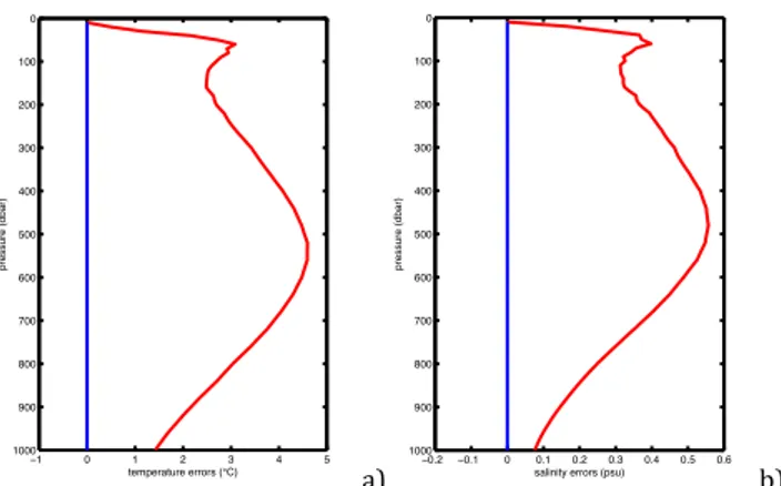
Conversely, only about 0.3 % of the variance is explained by the second mEOF mode. However, some important in-formation is still contained in the second mode. In fact, we also ran a single mode mEOF(T-S-SH) reconstruction (both for temperature and salinity) which gave much worse results than the mEOF-r in the two mode configurations (see Fig. 5). Actually,T andSpatterns in the first mEOF mode have the same sign, meaning that the surface anomalies with respect to the mean profile driven by this mode reflect down to the deep layers. On the contrary, the second mode basically accounts for the presence ofT andSanomalies only in the upper lay-ers, which might be related to the presence/absence of waters of coastal/riverine origin. More investigations will be needed to better understand which process drives the variability of this second mode. Meanwhile, it is clear that the third mode is related to conditions that apply to an extremely low num-ber of profiles. Adding it to the reconstruction, in fact, leads to the typical errors associated with model over-fitting. Only the best performing techniques, as evaluated with the previ-ous hindcast validation, have been applied to the SST, SSS and adjusted ADT maps for our study in the Gulf Stream area.
Considering the results of the tests presented in this section, the selected techniques are the mEOF-r(T-S -SH)SST-SSHand mEOF-r(T-S-SH)SSS-SSH.
4.3 Synthetic ARMOR3D and mEOF-r comparison
The newT andSsynthetic fields described in Sects. 4.1 and 4.2 have been compared: four are based on the ARMOR3D algorithm (three using only Reynolds L4, OSTIA L4 and ODYSSEA L4 SST as input, and one using ODYSSEA L4 SST and MESCLA HR SSS), and one is based on mEOF-R (using ODYSSEA L4 SST and MESCLA HmEOF-R SSS as in-put). The choice of using only ODYSSEA L4 in combination with MESCLA HR SSS for the highest resolution tests was driven, on one hand, by the fact that ODYSSEA is among the highest resolution Global SST L4 available and quality con-trolled operationally (see also Dash et al., 2010; Maturi et al., 2010) and, on the other hand, by the fact that it is the same product used to retrieve the high resolution SSS by Buon-giorno Nardelli (2012).
a) b) c) d)
Fig. 2a.Hindcast temperature mean bias errors (blue) and standard deviation errors (red) for different configurations of the mEOF-r technique
(see text for the details):(a)mEOF-r(T-S-SH),(b)mEOF-r(T-S-SH)SST-SSH,(c)mEOF-r(T-S-SH)SSS-SSHand(d)mEOF-r(T-SH).
a) b) c) d)
Fig. 2b.Hindcast salinity mean bias errors (blue) and standard deviation errors (red) for different configurations of the mEOF-r technique
(see text for the details):(a)mEOF-r(T-S-SHH),(b)mEOF-r(T-S-SH)SST-SSH,(c)mEOF-r(T-S-SH)SSS-SSHand(d)mEOF-r(S-SH).
a) b) c)
−0.1 −0.05 0 0.05 0.1 0
100 200 300 400 500 600 700 800 900 1000
pressure (dbar)
SH mEOF modes mode 1 mode 2 mode 3
−0.3−0.25−0.2−0.15−0.1−0.05 0 0.05 0.1 0
100
200
300
400
500
600
700
800
900
1000
pressure (dbar)
S mEOF modes
mode 1 mode 2 mode 3
−0.2−0.15−0.1−0.05 0 0.05 0.1 0.15 0.2 0
100
200
300
400
500
600
700
800
900
1000
pressure (dbar)
T mEOF modes mode 1 mode 2 mode 3
Fig. 3.First three trivariate (T-S-SH) mEOF modes for the Gulf
Stream area computed from Argo profiles (see text):(a)steric height
component,(b)salinity component and(c)temperature component.
euphotic layer in the Gulf Stream area (Oschlies and Garc¸on, 1998).
The analysis has been performed both qualitatively, i.e. looking at spatial gradients and at the way the different features are resolved/projected at depth, and quantitatively, by estimating and comparing the zonal power spectra, de-fined similarly to Reynolds and Chelton (2010), for each of the products. To compute the spatial spectra at each lat-itude reducing the spectral leaking, a Blackman–Harris win-dowing has been applied prior before computing the fast Fourier transform. Moreover, as the windowing attenuates the overall signal power, the spectra have been scaled with
−1 −0.5 0 0.5 1
−1000
−900
−800
−700
−600
−500
−400 −300
−200
−100 0
Depth (m)
Baroclinic Vertical Normal Modes
BC mode 1 BC mode 2 BC mode 3
Fig. 4.Quasi-geostrophic normal modes computed from the mean
a) b)
−1 0 1 2 3 4 5
0
100
200
300
400
500
600
700
800
900
1000
pressure (dbar)
temperature errors (°C) HINDCAST mEOF−R
−0.2 −0.1 0 0.1 0.2 0.3 0.4 0.5 0.6 0
100
200
300
400
500
600
700
800
900
1000
pressure (dbar)
salinity errors (psu)
HINDCAST mEOF−R
Fig. 5.Hindcast temperature(a)and salinity(b)mean bias errors (blue) and standard deviation errors (red) when using only the first
mode in the mEOF-r trivariate reconstructions:(a)mEOF-r(T-S
-SH)SST-SSH,(b)mEOF-r(T-S-SH)SSS-SSH.
corresponding coherent power gains to make them compara-ble (Harris, 1978). The spectra obtained for each latitudinal band have been finally averaged in a single spectrum for each product.
Starting from the analysis of the temperature fields at the surface, Ostia SST has the lowest energy levels at all spa-tial frequencies (namely the lowest variance), and displays a ‘red spectrum’ behaviour until reaching an almost flat re-sponse at approximately 1 / 4◦ resolution, though its nomi-nal resolution is the highest among the products considered (1 / 20◦) (Fig. 8). This is coherent with the smooth
appear-ance of the SST field as evidenced in Fig. 7. Conversely, Odyssea SST and Reynolds SST display much higher power (more than one order of magnitude) at frequencies higher than 10−1(deg−1) and up to their Nyquist frequency (i.e. at characteristic lengths between approximately 1000 km and 25 km/50 km, respectively), even if both of them also reach an almost flat plateau at scales smaller than 1 / 4◦(though if keeping a higher energy content than Ostia). Odyssea SST very clearly displays the highest energy in the spatial range between 100 km and 25 km, and the smallest spatial features: the Gulf Stream core is visible as a thin warm tongue off-shore Cape Hatteras and several small scale features are ob-served along the main flow. Even if some of these might be considered quite “noisy”, most of them are clearly related to mesoscale features (e.g. the small cold core cyclonic eddy centered at 40◦N 53◦W).
The deep (100 m) synthetic temperature fields generally reflect the spatial characteristics of the surface input data, but the ARMOR3D and mEOF-r also have a different impact on the way the surface scales are projected in the deep fields. In particular, ARMOR3D synthetic field displays smoother structures than those visible in the corresponding mEOF-r field, even when using Odyssea SST as input. The corre-sponding power spectrum gets closer to the Ostia/Reynolds
ARMOR3D spectrum, while mEOF-r spectrum at 100 m dis-plays basically the same features as the corresponding SST, except for a slightly higher energy at the scales smaller than 1 / 4◦.
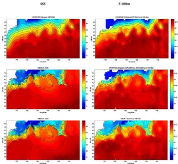
Concerning the salinity field, it has to be stressed that MESCLA HR-SSS and the ARMOR3D SSS fields are very different, as the latter is computed by combining a clima-tological first guess and the covariance between altimeter SLA and salinity (Fig. 9). More in detail, the MESCLA HR-SSS field shows a very sharp gradient and several small scale meanders all along the front of the Gulf Stream, with much fresher SSS than those present in the ARMOR3D field, which appears quite uniform and smooth. Corresponding SSS spectra display very different energy content below ap-proximately 300 km, down to the Nyquist spatial frequency. Both the mEOF-r and the ARMOR3D salinity reconstruction methods propagate the sharp gradient and the small scale fea-tures retrieved by MESCLA HR SSS down to 100 m, while the standard ARMOR3D field displays a much smoother pat-tern. Similar to what was found for the synthetic temperature fields, ARMOR3D vertical projection, however, significantly reduces the energy in the spatial frequency range below 10−1 (deg−1)(Fig. 10). Again, mEOF-r keeps basically the same energy down to 100 m, even with a slight increase at spa-tial scales below 10−1(deg−1), and a slight decrease at the longer wavelengths. The higher energy level at scales below 1 / 3◦ (where a plateau is again present) might anyway be considered as an indication of a too noisy reconstruction.
A preliminary evaluation of the vertical accuracy of the synthetic mEOF-r and ARMOR3D products has also been roughly performed via a weekly matchup comparison, which means that the in situ profiles collected in a temporal range of±3 days (weekly matchups) have been taken aside as an independent test dataset, and have been compared with the co-located profiles obtained with the different reconstruc-tion methods. The matchup comparison has the advantage of starting from fully independent surface input data, but the number of in situ profiles available within this weekly win-dow was too low to provide a significant estimate (actually, only 13 matchups were found). In fact, all error profiles esti-mated from the high resolution surface input produced equiv-alent results (within a 1 sigma confidence level, estimated through bootstrapping). The estimated MBE and STDE are shown in Fig. 6. However, a longer test period should be used to get a real validation, and the estimated difference can pos-sibly also be affected by the temporal variability at scales shorter than 3 days, which might not be negligible in rapidly evolving frontal areas.
5 QG Vertical velocity estimation
a) b)
Fig. 6.Weekly comparison of temperature and salinity profiles from
mEOF-r and and synthetic ARMOR3D using Odyssea SST(a)and
MESCLA SSS(b).
Fig. 7.SST (left panels) and temperature at 100 m (right panels) from the four reconstruction methods selected (from top to bottom): ARMOR3D using Reynolds L4 SST as input, ARMOR3D using OSTIA L4 SST as input, ARMOR3D using ODYSSEA L4 SST as
input, and mEOF-r(T-S-SH)SST-SSH.
than horizontal ones, and consequently they are not eas-ily measured through direct observations (e.g. Klein and Lapeyre, 2009; Frajka-Williams et al., 2011). Various in-direct methodologies have thus been proposed to estimate vertical velocity from observed density and geostrophic
ve-
a) b)
10−1
100
101
10−8
10−6
10−4
10−2
100
102
spatial frequency (deg−1)
Power Spectral Density
SST Zonal Spectra
Synthetic Armor3D OSTIA Synthetic Armor3D Odyssea Synthetic Armor3D Reynolds
mEOF−r
10−1
100
101 10−8
10−6 10−4 10−2 100 102
spatial frequency (deg−1)
Power Spectral Density
T (100m) Zonal Spectra
Synthetic Armor3D OSTIA Synthetic Armor3D Odyssea Synthetic Armor3D Reynolds mEOF−r
Fig. 8.Zonal wavenumber spectra computed from the reconstructed
temperature fields at the surface(a)and at 100 m depth(b).
Fig. 9.SSS (left panels) and salinity at 100 m (right panels) from the three reconstruction methods selected (from top to bottom): ARMOR3D using ODYSSEA L4 SST as input, ARMOR3D using
ODYSSEA L4 SST and MESCLA SSS as input, and mEOF-r(T-S
-SH)SSS-SSH.
locity fields. Though more complicated techniques such as the semi-geostrophic omega equation (Vi´udez and Dritchel, 2004) have been proposed, the most used technique is based on the solution of the quasi-geostrophic (QG) omega equa-tion (e.g. Tintor´e et al., 1991; Buongiorno Nardelli et al., 2001; Pascual et al., 2004; Ruiz et al., 2009), which has al-ready been shown to give reasonable estimates of the vertical velocities compared to primitive equation models (Pinot et al., 1996).
5.1 Qvector formulation of the omega equation
a) b)
10−1 100 101
10−8 10−6 10−4 10−2 100 102
spatial frequency (deg−1)
Power Spectral Density
SSS Zonal Spectra
Synthetic Armor3D Synthetic Armor3D SSS mEOF−r
10−1 100 101
10−8
10−6
10−4
10−2
100
102
spatial frequency (deg−1)
Power Spectral Density
S (100m) Zonal Spectra Synthetic Armor3D Synthetic Armor3D SSS mEOF−r
Fig. 10. Zonal wavenumber spectra computed from the
recon-structed salinity fields at the surface(a)and at 100 m depth(b).
et al., 2004; Ruiz et al., 2009) was adapted to the specific products considered.
Actually, the omega equation requires as input both the geostrophic field and the density stratification. The geostrophic currents have been estimated referencing the thermal wind estimates to the absolute surface altimeter ve-locities (when applied to observation-based products, see also Mulet et al., 2012). Two reference levels for dynamic height computation are considered for models: the surface and 1000 m depth. The code is derived from the QG vorticity and thermodynamic equation (Hoskins et al., 1978):
∇2N2w+f2∂
2w
∂z2 =2∇ ·Q
and
Q=
f
∂V
∂x ∂U
∂z +
∂V ∂y
∂V ∂z
−f
∂U
∂x ∂U
∂z +
∂U ∂y
∂V ∂z
,
where (U, V) are the geostrophic velocity components,N is the Brunt–V¨ais¨al¨a frequency andf the Coriolis parameter. In this implementation, N only depends on depth. Differ-ent boundary conditions have been tested (i.e. Dirichelet and Neumann conditions), however, given the elliptic nature of the omega equation, no significant differences were found a few grid points away from the boundaries in the two cases.
5.2 Comparison of the MyOcean model PE and QG
vertical velocities
To evaluate the accuracy of the quasi-geostrophic approxima-tion, the QG vertical velocities (qgw) obtained by applying the omega equation were compared to the Mercator Oc´ean model output based on primitive equation solutions. The im-pact of the resolution has been assessed through two tests: comparing the QG vertical velocity obtained from the origi-nal model fields at 1 / 4◦and 1 / 12◦resolution and compar-ing the QG velocities estimated after subsamplcompar-ing the 1 / 12◦ model fields at 1 / 4◦. The sensitivity to the choice of the reference level on the geostrophic and ageostrophic (vertical component) velocities has also been investigated.
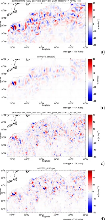
a)
b)
c)
d)
Fig. 11.Vertical velocity fields at 110 m as obtained from
primi-tive equation(a, c)and quasi-geostrophic omega equation(b, d)for
PSY3 1 / 4◦(a, b)and PSY2 1 / 12◦(c, d)Mercator models.
a) b) c)
Fig. 12.Scatter plot between vertical velocity fields at 110 m as obtained from primitive equation and quasi-geostrophic omega equation for
(a)PSY3 (1 / 4◦) Mercator model,(b)PSY2 (1 / 12◦) Mercator model interpolated onto a 1 / 4◦regular grid, and(c)PSY2 (1 / 12◦) Mercator
model.
between PE (Pearson coefficient) and QG vertical velocity patterns shows a reasonable agreement in both model simu-lations, even if model QG vertical velocity values underes-timate the PE velocities at low resolution. These differences can be better quantified looking at the scatter plot and com-puting correlation coefficients, as displayed in Fig. 12 (sim-ilar results were also found for deeper layers, not shown). In fact, QG velocities displayed maximum upward and downward values of the order of 40–60 m day−1 and 10– 15 m day−1 in the high resolution and low resolution tests, with correlation with PE reaching almost 0.8 and 0.7, respec-tively. The test of re-interpolating the PSY2 data (using bilin-ear interpolation) on the 1 / 4◦grid showed that bothwfields (QG and PE) are dramatically reduced by the interpolation, so that the final results are similar to what was obtained with PSY3 (Fig. 12).
The results thus indicate that resolution is a key factor in the estimate of the vertical component of the ageostrophic velocity through the quasi-geostrophic omega (compared to PE estimates). If sufficient resolution is kept, velocities are more correctly reproduced even in the quasi-geostrophic ap-proximation, and even though the patterns in the QG solution may be slightly smoother, the estimated values compare rea-sonably well. In the following, the QG method will thus be applied to the observation-based synthetic 3-D products, pro-viding a fully observational estimate of the vertical velocities for the test case.
5.3 Vertical velocities estimates from observation-based 3-D products
As expected, the quasi-geostrophic vertical velocities ob-tained from the synthetic fields increase significantly when increasing the grid resolution. A qualitative comparison of theqgwretrieved by applying the omega equation to the syn-thetic ARMOR3D products and mEOF-r fields is thus illus-trated in Fig. 13. The lowest velocities were estimated from the synthetic ARMOR3D using the Reynolds L4 SST (peak
qgw∼32 m day−1, horizontal velocities peak∼1.5 m s−1).
On the other hand, the synthetic ARMOR3D qgw com-puted from OSTIA, namely at the highest nominal resolu-tion, do not display the highest average and peak veloci-ties. This is not surprising considering the effective reso-lution of the tracer fields is lower (see Sect. 4.3). How-ever, coherent with the findings of the Sect. 5.2, they dis-play higher values than those obtained from Reynolds (peak
qgw∼52 m day−1, peak horizontal velocities∼1.7 m s−1). Slightly higher values were computed from synthetic AR-MOR3D using Odyssea SST as input, with peak qgw
values of ∼54 m day−1 and peak horizontal velocities of ∼1.7 m s−1. The most intense velocities, however, were
Synthetic ARMOR3D – Reynolds ¼°
a) Synthetic ARMOR3D – Ostia 1/20°
b) Synthetic ARMOR3D – Odyssea 1/10°
c) Synthetic ARMOR3D – Odyssea 1/10° + MESCLA SSS
d) mEOF‐r – Odyssea 1/10° + MESCLA SSS
e)
Fig. 13.QG vertical velocity fields at 100 m as retrieved from the temperature
and salinity fields reconstructed through the selected methods:(a)ARMOR3D using
Reynolds L4 SST as input,(b)ARMOR3D using OSTIA L4 SST as input,(c)
AR-MOR3D using ODYSSEA L4 SST as input,(d)ARMOR3D using ODYSSEA L4 SST
and MESCLA SSS as input, and(e)mEOF-r(T-S-SH)SSS-SSHfor the salinity field and
mEOF-r(T-S-SH)SST-SSHfor the temperature.
Synthetic ARMOR3D – Reynolds ¼°
a)
Synthetic ARMOR3D – Ostia 1/20°
b)
Synthetic ARMOR3D – Odyssea 1/10°
c)
Synthetic ARMOR3D – Odyssea 1/10° + MESCLA SSS
d)
mEOF‐r – Odyssea 1/10° + MESCLA SSS
e)
Fig. 14.Zoom of the QG vertical velocity fields at 100 m as retrieved from the
tem-perature and salinity fields reconstructed through the selected methods:(a)ARMOR3D
using Reynolds L4 SST as input,(b)ARMOR3D using OSTIA L4 SST as input,(c)
ARMOR3D using ODYSSEA L4 SST as input,(d)ARMOR3D using ODYSSEA L4
SST and MESCLA SSS as input, and(e)mEOF-r(T-S-SH)SSS-SSHfor the salinity
field and mEOF-r(T-S-SH)SST-SSHfor the temperature. SSH isolines are
technique used, all the synthetic QG estimates gave the same upwelling/downwelling patterns, even if the strongest veloc-ities were retrieved from mEOF-r fields.
6 Conclusions
Within the MyOcean R&D project MESCLA, a step towards a more efficient combination and more complex analysis of existing observations has been made. MESCLA tested in-novative methods for the high resolution mapping of 3-D mesoscale dynamics from a combination of in situ and satel-lite data (as described in Sect. 4), developing new products that might be used as prototypes to gradually build the next generation of operational observation-based products. In or-der to demonstrate the new techniques’ potentials, ent estimates of the vertical velocities derived from differ-ent 3-D synthetic fields through a quasi-geostrophic diag-nostic model have been compared (Sect. 5). Resolution con-firmed to be an important factor for the retrieval of the cur-rents. However, even within the limits of a simplified dynam-ical framework, and knowing that most of the analysis could not necessarily go beyond a simple qualitative comparison (vertical velocities cannot be measured directly at sea), re-alistic estimates of the vertical field could be retrieved, at least as compared to those diagnosed through primitive equa-tion numerical models. The ocean observaequa-tion-based prod-ucts tested within MESCLA might thus open a wide range of possible applications for both operational oceanography and ocean climate monitoring studies.
Acknowledgements. This work was carried out in the framework of the MESCLA (MEsoSCaLe dynamical Analysis) project,
funded within the MyOcean Call for R&D Proposals (2010–
2012, Mercator Ocean Ref. PB-LC 10-103). MyOcean project (development and pre-operational validation of GMES Marine Core Services (2009–2012) has been funded within the call EU FP7-SPACE-2007-1 (Grant Agreement nr. 218812).
Edited by: P.-Y. Le Traon
References
Allen, J. T. and Smeed, D. A.: Potential vorticity and vertical ve-locity at the Iceland-Færœs front, J. Phys. Oceanogr., 26, 2611– 2634, 1996.
Autret, E. and Pioll´e, J. F.: Implementation of a global SST analysis, MERSEA-WP02-IFR-STR-001-1A report, 2007.
AVISO: Ssalto/Duacs userHandbook: (M)SLAand(M)ADT near-real time and delayed time products, SALP-MU-P-EA-21065-CLS, Edn. 3.0, 68 pp., 2012.
Barnier, B., Madec, G., Penduff, T., Molines, J. M., Treguier, A. M., Le Sommer, J., Bekmann, A., Biastoch, A., Boning, C., Dengg, J., Derval, C., Durand, E., Gulev, S., Remy, E., Talandier, C., Theeten, S., Maltrud, M., McClean, J., and De Cuevas, B.: Impact of partial steps and momentum advection schemes in
a global ocean circulation model at eddy-permitting resolution, Ocean Dynam., 56, 543–567, 2006.
Bower, A. S.: Potential Vorticity Balances and Horizontal Diver-gence along Particle Trajectories in Gulf Stream Meanders East of Cape Hatteras, J. Phys. Oceanogr., 19, 1669–1681, 1989. Bower, A. S. and Rossby, T.: Evidence of cross-frontal exchange
processes in the Gulf Stream based on isopycnal RAFOS float data, J. Phys. Oceanogr., 19, 1177–1190, 1989.
Bretherton, F. P., Davis, R. E., and Fandry, C. B.: A technique for objective analysis and design of oceanographic experiments ap-plied to MODE-73, Deep-Sea Res. Pt. I, 23, 559–582, 1976. Buongiorno Nardelli, B.: A novel approach to the high resolution
interpolation of in situ Sea Surface Salinity, J. Atmos. Ocean. Tech., 29, 867–879, doi:10.1175/JTECH-D-11-00099.1, 2012. Buongiorno Nardelli, B. and Santoleri, R.: Reconstructing synthetic
profiles from surface data, J. Atmos. Ocean. Tech., 21, 693–703, 2004.
Buongiorno Nardelli, B. and Santoleri, R.: Methods for the recon-struction of vertical profiles from surface data: multivariate anal-yses, residual GEM and variable temporal signals in the North Pacific Ocean, J. Atmos. Ocean. Tech., 22, 1763–1782, 2005. Buongiorno Nardelli, B., Sparnocchia, S., and Santoleri, R.: Small
mesoscale features at a meandering upper ocean front in the western Ionian Sea (Mediterranean Sea): vertical motion and po-tential vorticity analysis, J. Phys. Oceanogr., 31, 8, 2227–2250, 2001.
Buongiorno Nardelli, B., Cavalieri, O., Rio, M.-H., and Santoleri, R.: Subsurface geostrophic velocities inference from altimeter data: application to the Sicily Channel (Mediterranean Sea), J. Geophys. Res., 111, C04007, doi:10.1029/2005JC003191, 2006. Carnes, M. R., Teague, W. J., and Mitchell, J. L.: Inference of sub-surface thermohaline structure from fields measurable by satel-lite, J. Atmos. Ocean. Tech., 11, 551–566, 1994.
Cushman-Roisin, B.: Introduction to Geophysical Fluid Dynamics, Prentice Hall, 1994.
Dash, P., Ignatov, A., Kihai, Y., and Sapper, J.: The SST Qual-ity Monitor (SQUAM), J. Atmos. Ocean. Tech., 27, 1899–1917, doi:10.1175/2010JTECHO756.1, 2010.
Dhomps, A.-L., Guinehut, S., Le Traon, P.-Y., and Larnicol, G.: A global comparison of Argo and satellite altimetry observations, Ocean Sci., 7, 175–183, doi:10.5194/os-7-175-2011, 2011. Dombrowsky, E., Bertino, L., Brassington, G. B., Chassignet, E.
P., Davidson, F., Hurlburt, H. E., Kamachi, M., Lee, T., Martin, M. J., Mei, S., and Tonani, M.: GODAE systems in operation, Oceanography, 22, 80–95, doi:10.5670/oceanog.2009.68, 2009. Donlon, C. J., Martin, M., Stark, J. D., Roberts-Jones, J., Fiedler, E.,
and Wimmer, W.: The Operational Sea Surface Temperature and Sea Ice analysis (OSTIA), Remote Sens. Environ., 116, 140–158, doi:10.1016/j.rse.2010.10.017, 2011.
Fox, D. N., Teague, W. J., Barron, C. N., Carnes, M. R., and Lee, C. M.: The modular ocean data assimilation system (MODAS), J. Atmos. Ocean. Tech., 19, 240–252, 2002.
Frajka-Williams, E., Eriksen, C. C., Rhines, P. B., and
Harcourt, R. R.: Determining Vertical Water Velocities from Seaglider, J. Atmos. Ocean. Tech., 28, 1641–1656, doi:10.1175/2011JTECHO830.1, 2011.
Gavart, M. and De Mey, P.: Isopycnal EOFs in the Azores Current region: A statistical tool for dynamical analysis and data assimi-lation, J. Phys. Ocean., 27, 2146–2157, 1997.
Guinehut, S., Le Traon, P. Y., Larnicol, G., and Philipps, S.: Com-bining Argo and remote-sensing data to estimate the ocean three-dimensional temperature fields – a first approach based on simu-lated observations, J. Mar. Sys., 46, 85–98, 2004.
Guinehut, S., Le Traon, P.-Y., and Larnicol, G.: What can we learn from Global Altimetry/Hydrography comparisons?, Geo-phys. Res. Lett, 33, L10604, doi:10.1029/2005GL025551, 2006. Guinehut, S., Dhomps, A.-L., Larnicol, G., and Le Traon, P.-Y.: High resolution 3-D temperature and salinity fields derived from in situ and satellite observations, Ocean Sci., 8, 845–857, doi:10.5194/os-8-845-2012, 2012.
Harris, F. J.: On the use of Windows for Harmonic Analysis with the Discrete Fourier Transform, P. IEEE, 66, 51–83, 1978. Hoskins, B. J., Draghici, I., and Davies, H. C.: A new look at the
omega-equation, Q. J. Roy. Meteorol. Soc., 104, 31–38, 1978. Ingleby, B. and Huddleston, M.: Quality control of ocean
tempera-ture and salinity profiles – historical and real-time data, J. Mar. Sys., 65, 158–175, doi:10.1016/j.jmarsys.2005.11.019, 2007. Isern-Fontanet, J., Lapeyre, G., Klein, P., Chapron, B., and Hecht,
M. W.: Three-dimensional reconstruction of oceanic mesoscale currents from surface information, J. Geophys. Res., 113, C09005, doi:10.1029/2007JC004692, 2008.
Joyce, T. M., Thomas, L. N., and Bahr, F.: Wintertime observations of Subtropical ModeWater formation within the Gulf Stream, Geophys. Res. Lett., 36, L02607, doi:10.1029/2008GL035918, 2009.
Klein, P. and Lapeyre, G.: The oceanic vertical pump induced by mesoscale eddies, Annu. Rev. Mar. Sci., 351–375, 2009. Klein, P., Isern-Fontanet, J., Lapeyre, G., Roullet, G., Danioux,
E., Chapron, B., Le Gentil, S., and Sasaki, H.: Diagnosis of vertical velocities in the upper ocean from high resolu-tion sea surface height, Geophys. Res. Lett., 36, L12603, doi:10.1029/2009GL038359, 2009.
Larnicol, G., Guinehut, S., Rio, M.-H., Drevillon, M., Faugere, Y., and Nicolas, G.: The Global Observed Ocean Products of the French Mercator project, Proceedings of 15 Years of progress in Radar Altimetry Symposium, ESA Special Publication, SP-614, 2006.
Lellouche, J.-M., Le Galloudec, O., Dr´evillon, M., R´egnier, C., Greiner, E., Garric, G., Ferry, N., Desportes, C., Testut, C.-E., Bricaud, C., Bourdall´e-Badie, R., Tranchant, B., Benkiran, M., Drillet, Y., Daudin, A., and De Nicola, C.: Evaluation of real time and future global monitoring and forecasting systems at Merca-tor Oc´ean, Ocean Sci. Discuss., 9, 1123–1185, doi:10.5194/osd-9-1123-2012, 2012.
Lindstrom, S. S., Qian, X., and Watts, D. R.: Vertical motion in the Gulf Stream and its relation to meanders, J. Geophys. Res., 102, 8485–8503, 1997.
Madec, G.: “NEMO ocean engine”, Note du Pole de mod´elisation, Institut Pierre-Simon Laplace (IPSL), France, No 27 ISSN No 1288-1619, 2008.
Maturi, E., Harris, A., and Sapper, J.: A New Ultra High Resolution Sea Surface Temperature Analyses from GOES-R and NPOESS-VIIRS, 90th AMS Annual Meeting, 6th Annual Symposium on Future National Operational Environmental Satellite Systems-NPOESS and GOES-R, 17–21 January 2010, Atlanta, Georgia,
2010.
Meinen, C. S. and Watts, D. R.: Vertical structure and transport on a transect across the North Atlantic Current near 42 degrees N: time series and mean, J. Geophys. Res., 105, 21869–21891, 2000.
Mitchell, D. A., Wimbush, M., Watts, D. R., and Teague, W. J.: The Residual GEM technique and its application to the Southwestern Japan/East Sea, J. Atmos. Ocean. Tech., 21, 1895–1909, 2004. Mulet, S., Rio, M.-H., Mignot, A., Guinehut, S., and Morrow, R.:
A new estimate of the global 3D geostrophic ocean circulation based on satellite data and in situ measurements, Deep Sea Res. Pt. II, 77, 70–81, doi:10.1016/j.dsr2.2012.04.012, 2012. Oschlies, A. and Garcon, V.: Eddy-induced enhancement of primary
production in a model of the North Atlantic Ocean, Nature, 394, 266–269, 1998.
Pascual, A. and Gomis, D.: Use of Surface Data to Estimate Geostrophic Transport, J. Atmos. Ocean. Tech., 20, 912–926, 2003.
Pascual, A., Gomis, D., Haney, R. H., and Ruiz, S.: A quasi-geostrophic analysis of a meander in the Palam´os Canyon: verti-cal velocity, geopotential tendency and a relocation technique, J. Phys. Oceanogr., 34, 2274–2287, 2004.
Pinot, J.-M., Tintor´e, J., and Wang, D.-P.: A study of the omega equation for diagnosing vertical motions at ocean fronts, J. Mar. Res., 54, 239–259, 1996.
Reynolds, R. W. and Chelton, D. B.: Comparisons of daily sea sur-face temperature analyses for 2007–08, J. Climate, 23, 3545– 3562, 2010.
Reynolds, R. W., Smith, T. M., Liu, C., Chelton, D. B., Casey, K. S., and Schlax, M. G.: Daily high-resolution blended analyses for sea surface temperature, J. Climate, 20, 5473–5496, 2007. Roemmich, D. and Gilson, J.: The 2004–2008 mean and annual
cy-cle of temperature, salinity and steric height in the global ocean from the Argo program, Prog. Oceanogr., 82, 81–100, 2009. Ruiz, S., Pascual, A., Garau, B., Pujol, I., and Tintor´e, J.: Vertical
motion in the upper ocean from glider and altimetry data, Geo-phys. Res. Lett., 36, L14607, doi:10.1029/2009GL038569, 2009. Stammer, D., K¨ohl, A., Awaji, T., Balmaseda, M., Behringer, D., Carton, J., Ferry, N., Fischer, A., Fukumori, I., Giese, B., Haines, K., Harrison, E., Heimbach, P., Kamachi, M., Keppenne, C., Lee, T., Masina, S., Menemenlis, D., Ponte, R., Remy, E., Rienecker, M., Rosati, A., Schr¨eoter, J., Smith, D., Weaver, A., Wunsch, C., and Xue, Y.: Ocean Information Provided through Ensemble Ocean Syntheses, in: Proceedings of OceanObs’09: Sustained Ocean Observations and Information for Society, edited by: Hall, J., Harrison, D. E., and Stammer, D., Vol. 2, Venice, Italy, 21–25 September 2009, ESA Publication WPP-306, 2010.
Thomas, L. N. and Joyce, T. M.: Subduction on the Northern and Southern Flanks of the Gulf Stream, J. Phys. Oceanogr., 40, 429– 438, doi:10.1175/2009JPO4187.1, 2010.
Tintor´e, J., Gomis, D., Alonso, S., and Parrilla, G.: Mesoscale
dynamics and vertical motion in the Alboran Sea,
J. Phys. Oceanogr., 21, 811–823, doi:
10.1175/1520-0485(1991)021<0811:MDAVMI>2.0.CO;2, 1991.
Vi´udez, A. and Dritschel, D. G.: Potential Vorticity and the Quasigeostrophic and Semi30 geostrophic MesoscaleVertical Velocity, J. Phys. Oceanogr., 34, 865–887,
doi:10.1175/1520-0485(2004)034<0865:PVATQA>2.0.CO;2, 2004.
Von Schuckmann, K., Gaillard, F., and Le Traon, P.-Y.: Global hy-drographic variability patterns during 2003–2008, J. Geophys. Res., 114, C09007, doi:10.1029/2008JC005237, 2009.
Watts, D. R., Sun, C., and Rintoul, S.: A Two-Dimensional Gravest Empirical Mode Determined from Hydrographic Observations in the Subantarctic Front, J. Phys. Oceanogr., 31, 2186–2209, 2001.
Wong, A., Keeley, R., Carval, T., and the Argo Data Manage-ment Team: Argo quality control manual, V2.6, available at: http://www.argodatamgt.org/content/download/341/2650/file/ argo-quality-control-manual-V2.6.pdf, 2012.