The role of horizontal model resolution in assessing the transport of CO in a middle latitude cyclone using WRF-Chem

(1)

ACPD

13, 14871–14925, 2013

Transport of CO in a middle latitude

cyclone

C. A. Klich and H. E. Fu-elberg

Title Page

Abstract Introduction

Conclusions References

Tables Figures

◭ ◮

Back Close

Full Screen / Esc

Printer-friendly Version Interactive Discussion

Discussion

P

a

per

|

Dis

cussion

P

a

per

|

Discussion

P

a

per

|

Discussio

n

P

a

per

Atmos. Chem. Phys. Discuss., 13, 14871–14925, 2013 www.atmos-chem-phys-discuss.net/13/14871/2013/ doi:10.5194/acpd-13-14871-2013

Atmospheric Chemistry and Physics

Open Access

Discussions

Geoscientiic Geoscientiic

This discussion paper is/has been under review for the journal Atmospheric Chemistry and Physics (ACP). Please refer to the corresponding final paper in ACP if available.

The role of horizontal model resolution in

assessing the transport of CO in a middle

latitude cyclone using WRF-Chem

C. A. Klich and H. E. Fuelberg

Department of Earth, Ocean and Atmospheric Science, Florida State University, Tallahassee, FL 32306-4520, USA

Received: 21 April 2013 – Accepted: 6 May 2013 – Published: 5 June 2013

Correspondence to: H. E. Fuelberg (hfuelberg@fsu.edu)

(2)

ACPD

13, 14871–14925, 2013

cyclone

Title Page

Tables Figures

◭ ◮

Back Close

Full Screen / Esc

Discussion

P

a

per

|

Dis

cussion

P

a

per

|

Discussion

P

a

per

|

Discussio

n

P

a

per

|

Abstract

We use the Weather Research and Forecasting with Chemistry (WRF-Chem) online chemical transport model to simulate a middle latitude cyclone in East Asia at three different horizontal resolutions (45, 15, and 5 km grid spacing). The cyclone contains a typical warm conveyor belt (WCB) with an embedded squall line that passes through an

5

area having large surface concentrations (>_{400 ppbv) of carbon monoxide (CO). Model}

output from WRF-Chem is used to compare differences between the large-scale CO vertical transport by the WCB (the 45 km simulation) with the smaller-scale transport due to its convection (the 5 km simulation). Forward trajectories are calculated from WRF-Chem output using HYSPLIT. At 45 km grid spacing, the WCB exhibits gradual

10

ascent, lofting surface CO to 6–7 km. Upon reaching the warm front, the WCB and associated CO ascend more rapidly and later turn eastward over the Pacific Ocean. Convective transport at 5 km resolution with explicitly resolved convection occurs much more rapidly, with surface CO lofted to altitudes greater than 10 km in 1 h or less. We also compute CO vertical mass fluxes to compare differences in transport due to the

15

different grid spacings. Upward CO flux exceeds 110 000 t h−1_{in the domain with}

ex-plicit convection when the squall line is at peak intensity, while fluxes from the two coarser resolutions are an order of magnitude smaller. Specific areas of interest within the 5 km domain are defined to compare the magnitude of convective transport to that within the entire 5 km region. Although convection encompasses only a small portion

20

of the 5 km domain, it is responsible for∼40 % of the upward CO transport. We also

examine the vertical transport due to a short wave trough and its associated area of convection, not related to the cyclone, that lofts CO to the upper troposphere. Results indicate that fine-scale resolution with explicitly resolved convection is important when assessing the vertical transport of surface emissions in areas of deep convection.

(3)

ACPD

13, 14871–14925, 2013

cyclone

Title Page

Tables Figures

◭ ◮

Back Close

Full Screen / Esc

Discussion

P

a

per

|

Dis

cussion

P

a

per

|

Discussion

P

a

per

|

Discussio

n

P

a

per

1 Introduction

Anthropogenic emissions are transported at atmospheric scales ranging from turbu-lence to global phenomena. Where and how these emissions are transported can have major impacts on air quality (e.g., Ellingsen et al., 2008) and can a_ffect radiative forc-ing and other physical and dynamical processes that impact Earth’s climate (e.g., Park

5

et al., 2001). Accurately modeling pollution transport is crucial to understanding atmo-spheric chemistry and its e_ffects on the environment.

Surface-based pollutants are transported most efficiently when they are lofted to the middle or upper troposphere where wind speeds generally are stronger than near the surface. Three primary mechanisms can loft pollutants from the boundary layer

10

to the free troposphere: 1) airstreams such as the warm conveyor belt (WCB) that are associated with middle latitude cyclones (Bey et al., 2001; Cooper et al., 2002; Hannan et al., 2003; Kiley and Fuelberg, 2006), 2) orographic lifting (Henne et al., 2004; Chen et al., 2009; Ding et al., 2009), and 3) deep convection (Lawrence et al., 2003; Liu et al., 2003; Hess, 2005; Halland et al., 2009; Zhao et al., 2009). Although all three transport

15

mechanisms are important, middle latitude cyclones and deep convection are the most variable and difficult to simulate accurately using meteorological or chemical transport models (CTMs).

Although middle latitude cyclones and their associated WCBs can occur virtually anywhere in the middle and polar latitudes (Stohl et al., 2002), distinct maxima are

20

located off the east coasts of North America and Asia (Stohl, 2001; Eckhardt et al., 2004). The long-range synoptic scale WCB-related transport of atmospheric pollutants has been studied across both the Pacific Ocean (e.g., Jaffe et al., 1999; Yienger et al., 2000; Bey et al., 2001; Carmichael et al., 2003; Heald et al., 2003; Jacob et al., 2003; Liu et al., 2003; Cooper et al., 2004) and Atlantic Ocean (Stohl and Trickl, 1999; Cooper

25

(4)

ACPD

13, 14871–14925, 2013

cyclone

Title Page

Tables Figures

◭ ◮

Back Close

Full Screen / Esc

Discussion

P

a

per

|

Dis

cussion

P

a

per

|

Discussion

P

a

per

|

Discussio

n

P

a

per

|

to the western United States (US) has been shown to increase local surface ozone concentrations (Jacob et al., 1999; Fiore et al., 2002; Jaffe et al., 2004; Oltmans et al., 2008; Zhang et al., 2008; Reidmiller et al., 2009; Lin et al., 2012). Asian emissions sometimes extend as far as Europe (Stohl et al., 2007; Fiedler et al., 2009).

A great deal of transport modeling has been done using global CTMs whose typical

5

grid spacing is approximately 2◦ _latitude

×2.5◦ longitude (Park et al., 2001; Liu et al.,

2003; Liang et al., 2004; Li et al., 2005). However, such coarse grid resolution can pro-duce deficiencies in the results. Large spatial gradients of tracer concentrations result from complex interactions between emissions, meteorological conditions, and nonlin-ear atmospheric chemistry (Constantinescu et al., 2008; Srivastava et al. 2001a, b).

10

Coarse grids artificially di_ffuse these large gradients, and coupled with highly nonlinear chemistry, may adversely affect the predicted pollutant concentrations. Furthermore, coarse resolution models excessively diffuse the concentrations of atmospheric pollu-tants, thereby underestimating their amounts in the upper troposphere (Heald et al., 2003; Lin et al., 2010).

15

In terms of resolving specific meteorological phenomena, coarse resolution mod-els capture large-scale transport processes such as the WCBs (Harrold, 1973) that originate in the warm sector of a cyclone and ascend ahead of the surface cold front (Carlson, 1980). These cyclones and their WCBs are thought to be the dominant form of synoptic scale transport in the middle latitudes (Harrold, 1973), and the primary

20

mechanism for rapidly exporting air pollution from Asia to North America (Cooper et al., 2002, 2004; Stohl et al., 2002)

Conversely, the meteorological conditions that influence the development of deep convection, such as mixing depth, local thermodynamic variability, and wind velocity are best resolved by models having much higher resolution than CTMs (Lin et al.,

25

(5)

ACPD

13, 14871–14925, 2013

cyclone

Title Page

Tables Figures

◭ ◮

Back Close

Full Screen / Esc

Discussion

P

a

per

|

Dis

cussion

P

a

per

|

Discussion

P

a

per

|

Discussio

n

P

a

per

the explicit resolution of convection requires a horizontal grid spacing less than∼5 km.

Lackmann (2011) recently recommended a grid spacing less than 4 km to achieve ex-plicit convective resolution. This recommendation is supported by recent studies such as Baldauf et al. (2011) and Weisman et al. (2008). We will use the term “explicit reso-lution” with the understanding that even a 4–5 km grid spacing is insu_fficient to resolve

5

all details of convection; cloud resolving models with grid spacings of a few meters are needed for that purpose.

Since convection is not ”explicitly” simulated in coarse resolution models, it must be parameterized using various cumulus parameterization schemes. There is uncertainty and subjectivity in selecting the best cumulus parameterization for a specific study.

10

However, the important point is that no parameterization scheme will provide the de-tailed representation provided by higher resolution models in which parameterization is not employed. Each scheme varies in its assumptions and methodology and may pro-duce considerably di_fferent results (Doherty et al., 2005; Taylor, 2011). Furthermore, it is not advisable to “turn off” convective parameterization and attempt to simulate

15

convection explicitly at coarse resolution because results have revealed slow forming, large convective storms that are not observed in nature (Weisman et al., 1997; Sato et al., 2008).

Many middle latitude cyclones have deep convection embedded in their WCBs. This embedded convection enhances the overall WCB transport, and may even exceed the

20

synoptic scale component in weaker cyclones (Purvis et al., 2003; Kiley and Fuelberg, 2006). During periods of summertime deep convection, as much as 50 % of pollutants in the boundary layer is transported to the free troposphere by thunderstorms (Thomp-son et al., 1994). Convection with strong updrafts can loft surface emissions to the tropopause (∼9–15 km altitude) as quickly as 30 min (Thompson et al., 1997).

Val-25

(6)

ACPD

13, 14871–14925, 2013

cyclone

Title Page

Tables Figures

◭ ◮

Back Close

Full Screen / Esc

Discussion

P

a

per

|

Dis

cussion

P

a

per

|

Discussion

P

a

per

|

Discussio

n

P

a

per

|

Few studies have quantified the differences in atmospheric chemical simulations that result from using relatively high versus lower resolution models. Lin et al. (2010) compared results from two high-resolution regional atmospheric chemistry models: the global Model for Ozone and Related Tracers (MOZART v2) (Horowitz et al., 2003) run at 1.9◦

×1.9◦ grid spacing, with the Weather Research and Forecasting with

Chem-5

istry (WRF-Chem) model (Grell et al., 2005) and the Community Multiscale Air Quality model (CMAQ) (Byun and Schere, 2006) run at 36×36 km grid spacing. Deep

con-vection was parameterized in both models. Results showed that the vertical lifting and outflow of Asian pollution were enhanced in the regional models throughout their study period. Nonetheless, 36 km grid spacing still is too coarse to resolve most aspects of

10

deep convection. Therefore, it is important to investigate vertical transport using even higher resolution models. A model grid spacing of 12 km produced the best agreement between simulated and measured concentrations of O3 and O3 precursors in Mexico City (Tie et al., 2010), with poorer performance at both larger and smaller spacing. Chock et al. (2002) concluded that coarse resolution leads to faulty representations

15

of ozone and nitrogen oxide chemistry. Similarly, simulated concentrations of particu-lates over central Europe agreed best with observations when the model grid spacing was 7 km instead of 28 km (Wolke et al., 2012). Using a high resolution (hundreds of meters) regional scale two-dimensional (2-D) model, Halland et al. (2009) found that a single squall line during its 8 h lifetime could transport as much as 96 metric tons (t_{) of} 20

CO upward and 67t_{downward at 300 hPa.}

This study focuses on the transport of CO within a middle latitude cyclone containing deep convection. We employ the WRF-Chem model run at horizontal grid spacings of 45, 15, and 5 km. Unlike Halland et al. (2009), we employ three-dimensional (3-D) sim-ulations to capture the full scope of convective transport. We compare transport based

25

(7)

ACPD

13, 14871–14925, 2013

cyclone

Title Page

Tables Figures

◭ ◮

Back Close

Full Screen / Esc

Discussion

P

a

per

|

Dis

cussion

P

a

per

|

Discussion

P

a

per

|

Discussio

n

P

a

per

Section 3 presents a synoptic overview, Sect. 4 the results, and Sect. 5 the summary and conclusions.

2 Data and methodology 2.1 Study domain

Our study domain encompassed a typical middle latitude cyclone in East Asia (Figs. 1–

5

2). A detailed synoptic overview is provided in Sect. 3. The simulations began at 00:00 UTC 22 May 2008 and ended five days later at 00:00 UTC 27 May, spanning the entire life cycle of the cyclone. Output from the first 12 h of the runs is not used in the discussions that follow to allow sufficient time for model spinup.

Model simulations were made using three nested domains (Fig. 1). The outer domain

10

(D1) covered most of eastern Asia with a horizontal grid spacing of 45 km. This rela-tively coarse spacing simulated large scale features of the cyclone such as its WCB. An embedded nested domain (D2) had a grid spacing of 15 km, and the innermost nested domain (D3) had a 5 km spacing that provided explicit resolution of deep con-vection embedded within the WCB. The wave cyclone was completely contained within

15

D2 during its life cycle (Fig. 2), and all important meteorological features were located far from the boundaries of D1 to reduce undesirable boundary effects (Warner et al., 1997). All three domains contained 50 sigma levels, most tightly packed in the bound-ary layer and near the tropopause.

2.2 Model specifics

20

(8)

ACPD

13, 14871–14925, 2013

cyclone

Title Page

Tables Figures

◭ ◮

Back Close

Full Screen / Esc

Discussion

P

a

per

|

Dis

cussion

P

a

per

|

Discussion

P

a

per

|

Discussio

n

P

a

per

|

is included near the model top of 50 hPa to prevent gravity waves from reflecting offthe upper boundary.

Meteorological initial and boundary conditions were obtained from the National Cen-ters for Environmental Protection (NCEP) final analysis on a 1◦

×1◦ grid at 26

pres-sure levels (http://dss.ucar.edu/datasets/ds083.2/). The boundary conditions were

up-5

dated every 6 h. Four-dimensional data assimilation (nudging) was used at 6 h inter-vals on the outer two domains. The recommended nudging coefficient (0.0003 s−1_,

Gilliam and Pleim, 2010) helped the simulations represent real-world conditions with-out being overly constrained. Other model settings and parameterizations are given in Table 1. An especially important choice was the Grell-3D cumulus parameterization

10

(ARW WRF User’s Guide, 2012) that is an updated version of the earlier Grell-Devenyi scheme (Grell and Devenyi, 2002). This parameterization, used only in D1 and D2, allows coarsely resolved subsidence to be spread to neighboring columns. Without this scheme, the downward motion between convective clouds is not well represented (Tzella and Legras, 2011). No cumulus parameterization was used in the 5 km domain,

15

i.e., the convection was explicitly resolved to the extent possible at 5 km grid spacing. WRF-Chem contains several options for simulating chemical interactions. We used the Regional Atmospheric Chemistry Mechanism (RACM) for gas phase chemistry that is based on the older Regional Acid Deposition Model, version 2 (RADM2, Stockwell et al., 1997). Although RACM simulates over 100 chemical species and their reactions, we

20

focus on CO due to its long residence time of approximately 1–2 months (e.g., Novelli et al., 1998). The Georgia Tech/Goddard Global Ozone Chemistry Aerosol Radiation and Transport (GOCART) aerosol parameterization (Chin et al., 2000) was used. GOCART is a bulk aerosol scheme that does not contain specific information about particle size or concentration, but instead calculates changes in total aerosol mass.

25

(9)

nest-ACPD

13, 14871–14925, 2013

cyclone

Title Page

Tables Figures

◭ ◮

Back Close

Full Screen / Esc

Discussion

P

a

per

|

Dis

cussion

P

a

per

|

Discussion

P

a

per

|

Discussio

n

P

a

per

ing, and the other only D1. These three simulations permitted an examination of the WCB, its convection, and the relationship between the two at both coarse and fine resolutions.

The Hybrid Single Particle Lagrangian Integrated Trajectory Model (HYSPLIT; Draxler and Hess, 1998; and http://ready.arl.noaa.gov/HYSPLIT.php) was used as a

5

complement to WRF-Chem to describe the different modes of transport over time. Us-ing the WRF-Chem simulations as input, HYSPLIT allowed us to create forward and backward trajectories at any starting location from any of the three simulations.

2.3 Emissions data

Several sets of emissions data were used to model the transport of CO. WRF-Chem

10

was initialized with chemical data from 4 (Emmons et al., 2010). MOZART-4 also was used to update WRF-Chem’s lateral boundary conditions at 6 h intervals. The archived data have a horizontal resolution of 1.9◦

×2.5◦ with 56 vertical levels.

Initial conditions also included biomass burning emissions from the Fire INventory from NCAR (FINN, Wiedinmyer et al., 2011). Anthropogenic source emissions were from

15

the Reanalysis of the TROpospheric dataset (RETRO, http://retro.enes.org). RETRO is a dataset of chemical composition at a resolution of 0.5◦

×0.5◦ that is mapped onto

the WRF-Chem grid using a program created by the Brazilian Centro de Previs ˜ao de Tempo e Estudos Clim ´aticos (CPTEC). Biogenic emissions were imported into WRF-Chem using the Model of Emissions of Gases and Aerosols from Nature (MEGAN,

20

Guenther et al., 2006). MEGAN is a high-resolution (∼1 km2) dataset that includes leaf

(10)

ACPD

13, 14871–14925, 2013

cyclone

Title Page

Tables Figures

◭ ◮

Back Close

Full Screen / Esc

Discussion

P

a

per

|

Dis

cussion

P

a

per

|

Discussion

P

a

per

|

Discussio

n

P

a

per

|

3 Case study

3.1 Synoptic overview

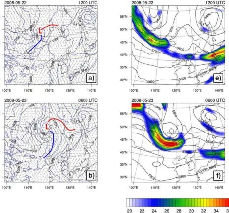
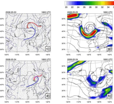
Our case study period (00:00 UTC 22 May–00:00 UTC 27 May 2008) focused on a typ-ical middle latitude cyclone over eastern Asia with a well defined WCB and associated deep convection (Fig. 2). The northeast part of D2 also included a separate

dissipat-5

ing low pressure system over the Sea of Okhotsk. The southwest parts of D1 and D2 encompassed the high terrain of the Himalayas. This section presents an overview of the synoptic, mesoscale, and surface CO characteristics during the life cycle of the major cyclone based on the WRF-Chem simulations. Later paragraphs will show that the simulations agree closely with observed conditions.

10

The surface low formed in eastern Mongolia near 12:00 UTC 22 May (Fig. 2a). It then moved slowly eastward into northeast China by 06:00 UTC 23 May (Fig. 2b), reaching its lowest central pressure of 992 hPa. After 12:00 UTC 23 May, the cyclone slowly weakened (Fig. 2c), and during the next 24 to 36 h (Fig. 2d) it gradually moved south-eastward along the border of northeast China and Russia while continuing to dissipate.

15

The frontal structure of the cyclone was typical. We manually located the warm, cold, and occluded fronts (Fig. 2a–d) using standard meteorological parameters from WRF-Chem. The surface cold front was characterized by a well defined wind shift from southwesterly ahead of the front to northwesterly behind, a strong gradient of dewpoint and temperature, and a low pressure trough. The cold front slowly moved eastward

20

with its parent low, eventually reaching the coast of northeast China (Fig. 2c). The warm front was less defined than the cold front. It moved little as the low slowly drifted eastward, and the system became occluded by 00:00 UTC 24 May (Fig. 2d).

Conditions at 500 hPa also were typical of middle latitude cyclones. A short wave trough deepened to form a closed low by 06:00 UTC 23 May (Fig. 2e–f) as wind speeds

25

increased to 40 m s−1 _{(Fig. 2f). Enhanced synoptic scale ascent southeast of the low}

(11)

ACPD

13, 14871–14925, 2013

cyclone

Title Page

Tables Figures

◭ ◮

Back Close

Full Screen / Esc

Discussion

P

a

per

|

Dis

cussion

P

a

per

|

Discussion

P

a

per

|

Discussio

n

P

a

per

intensified to create a well defined westerly jet stream. The low and associated jet weakened by 18:00 UTC 24 May (Fig. 2h).

The 500 hPa pressure level exhibited a second feature of interest (Fig. 2e–h). A short wave trough separate from the middle latitude cyclone began to develop over northeast China at 00:00 UTC 23 May with a wind maximum between 30◦_–35◦_{N and 115}◦_–120◦_E. 5

The trough slowly moved eastward, gradually increasing in strength. It approached the Pacific Coast by 18:00 UTC 23 May (Fig. 2g), and by 07:00 UTC 24 May winds east of the trough exceeded 25 m s−1 _{near southern Japan (Fig. 2h). The deep convection}

associated with the trough, as well as its flow patterns that produced CO transport are discussed in Sect. 4.

10

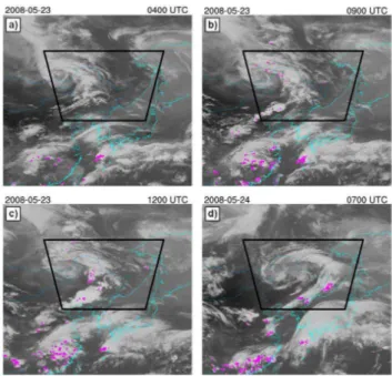
Our simulations closely represent the natural atmosphere. Observed infrared im-agery (Fig. 3) from the Multifunctional Transport Satellite (MTSAT-1R) is consistent with the simulations in Fig. 2. The cyclone exhibited a classic comma shaped cloud pattern. As the system intensified and eventually became occluded (Fig. 3b-d), the band of clouds ahead of the cold front became better defined, signifying the location of

15

the WCB described in Sect. 4. Similarly close agreements were found between other observed and simulated parameters, e.g., locations of the cyclone, its central pressure, and associated fronts (not shown).

3.2 Mesoscale features

Two major areas of deep convection occurred during the study period: a squall line

20

ahead of the surface cold front, and a multi-cellular complex over southeast China near the southern boundary of D1 (Fig. 3). The squall line ahead of the cold front formed near 02:00 UTC 23 May and dissipated just after 12:00 UTC 23 May. Although much of this modeled convection dissipated overnight (local time=UTC+8 h), some remnants of the squall line continued. Thunderstorm clusters re-generated ahead of the cold front

25

(12)

ACPD

13, 14871–14925, 2013

cyclone

Title Page

Tables Figures

◭ ◮

Back Close

Full Screen / Esc

Discussion

P

a

per

|

Dis

cussion

P

a

per

|

Discussion

P

a

per

|

Discussio

n

P

a

per

|

Lightning occurs when there is a deep layer of mixed phase hydrometeors, generally signifying tall clouds with vigorous updrafts. We used data from the World Wide Light-ning Location Network (WWLLN) to locate lightLight-ning flashes during the time of most intense convection. WWLLN has a detection efficiency of approximately 20 % in our study region (Rodger et al., 2009) and a location accuracy of 5–10 km (Rodger et al.,

5

2004). Despite this limited detection, previous studies have successfully used the data to locate deep convection (e.g., Abarca et al., 2010). WWLLN-derived lightning flashes were summed over 1 h periods between a half hour before and half hour after each satellite image and superimposed on the images (pink dots in Fig. 3). There was no lightning early in the morning of 23 May (Fig. 3a); however, high cloud tops and

light-10

ning developed within a few hours (Fig. 3b). The convection and its associated lightning continued for several hours (Fig. 3c) and dissipated late on 23 May. Less intense, dis-organized convection was simulated northwest of the surface low in the far northwest part of D3, consistent with the satellite imagery (Fig. 3b–c).

Comparisons of Figs. 3–4 reveal that locations of the WRF-Chem simulated deep

15

convection agree closely with those observed by satellite, again confirming the quality of the simulations. The squall line within D3 (Fig. 4) was located ahead of the surface cold front and exhibited simulated reflectivities exceeding 55 dBZ (Fig. 4b–c) when the maximum number of lightning flashes was observed (Fig. 3b–c). The line propagated from near the border of China and Mongolia to the border of China and Russia, a

20

distance of approximately 700 km. Strong updrafts and downdrafts accompanying the squall line produced vertical transport of boundary layer pollution that is described in Sect. 4.

The second major area of deep convection, multi-cell storms in southeast China just south of 30◦_{N, began near 04:00 UTC 23 May (Fig. 3a) and persisted through} 25

(13)

ACPD

13, 14871–14925, 2013

cyclone

Title Page

Tables Figures

◭ ◮

Back Close

Full Screen / Esc

Discussion

P

a

per

|

Dis

cussion

P

a

per

|

Discussion

P

a

per

|

Discussio

n

P

a

per

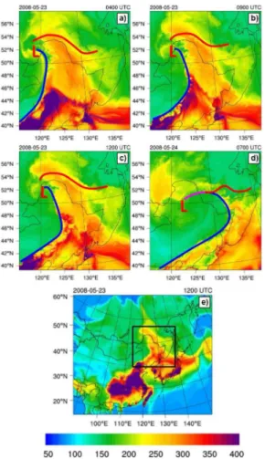
3.3 Surface CO

Eastern Asia contains some of the world’s greatest anthropogenic surface emissions (Richter et al., 2005; Ohara et al., 2007; Zhang et al., 2007, 2009). The greatest CO during our period (>_{400 ppbv) was located in domain D1, just south of D3 in eastern}

China (Fig. 5e). Some of the enhanced CO was advected into D3 by southerly winds

5

(Fig. 2), producing concentrations that exceed 400 ppbv over the extreme southern part of that smaller domain (Fig. 5a). The cyclonic flow transported CO northward, wrapping around the center of the low (Fig. 5a–c) after occlusion (Fig. 5d). The cold front was marked by a strong horizontal CO gradient (Fig. 5b–c), with air behind the front containing as much as 250 ppbv less CO than ahead. The horizontal gradient of

10

surface CO concentration across the warm front was not as great as with the cold front. The convection in southeast China within D1 (Fig. 3) occurred where CO concentra-tions exceeded 400 ppbv over a wide area (Fig. 5e). Since this area was located in the domain having 45 km grid spacing, the convection was parameterized, and Section 4 will show that its vertical transport of surface CO is relatively weak compared to that of

15

the explicitly resolved convection in D3.

The squall line in D3 influenced surface concentrations of CO (Fig. 5). Since con-vection rapidly lofts polluted boundary layer air to the free troposphere, surface CO beneath strong updrafts often is smaller than in surrounding areas. Additionally, down-drafts typically transport relatively small values of CO from the mid troposphere to the

20

surface. The effects of these convective scale vertical motions are apparent in Fig. 5b (40◦_{N, 120}◦_{E) and Fig. 5c (44}◦_{N, 125}◦_{E) as isolated areas of surface CO as small as}

150 ppbv, compared to surrounding environmental values exceeding 300 ppbv. When WRF-Chem was run at grid spacings greater than the 5 km in D3 (not shown), the fine-scale variations in CO concentration are not evident. Thus, high resolution models

25

(14)

ACPD

13, 14871–14925, 2013

cyclone

Title Page

Tables Figures

◭ ◮

Back Close

Full Screen / Esc

Discussion

P

a

per

|

Dis

cussion

P

a

per

|

Discussion

P

a

per

|

Discussio

n

P

a

per

|

4 Results

4.1 Parameterized convection at 45 km resolution

Simulations performed using only outer domain D1 (45 km resolution, Fig. 1) reveal synoptic scale aspects of the WCB and its transport of CO. We used WRF-Chem output from this single-domain simulation to calculate forward trajectories using HYSPLIT.

5

Areas of southwesterly surface winds far south of the parent low and just in advance of the cold front were considered the initiation area of the WCB, i.e., between 40◦_N–46◦_N

and 117◦_–126◦_{E (Fig. 6a). Trajectories were launched at each model grid point (45 km}

spacing) at 500 m above ground level. The trajectories were initialized at 06:00 UTC 23 May and continued for 48 h or until they left the model domain (Fig. 6a,c), the period

10

when the middle latitude cyclone and associated WCB were best developed (Fig. 5b). From this large number of trajectories, we isolated those representing the WCB by using criteria from Eckhardt et al. (2004). They required 48 h trajectories to travel eastward a distance exceeding 10◦_{longitude, northward at least 5}◦ _{latitude, and}

verti-cally at least 60 % of the average tropopause height at the ending latitude. The typical

15

tropopause height in our simulation region was 11–12 km, yielding a 48 h ascent crite-rion of at least 6.5 km. Applying these criteria isolated approximately 100 trajectories that represented the WCB (Fig. 6a,c).

The WCB derived from the 45 km grid spacing exhibits gradual ascent from the boundary layer to the free troposphere (Fig. 6c). It remains in the boundary layer ahead

20

of the cold front for the first 6 h (Fig. 6c) and then begins to ascend through the tropo-sphere, rising∼3 km. When it reaches the warm front near the border of eastern China

and southeast Russia (Fig. 6a), the ascent becomes more rapid, approximately 3 km during the next 6 h period. Once reaching the middle troposphere, the WCB turns more easterly (Fig. 6a). Maximum altitudes never exceed∼8 km (Fig. 6c).

25

The starting trajectory locations are in an area of enhanced CO (>_{400 ppbv, Fig. 5).}

(15)

ACPD

13, 14871–14925, 2013

cyclone

Title Page

Tables Figures

◭ ◮

Back Close

Full Screen / Esc

Discussion

P

a

per

|

Dis

cussion

P

a

per

|

Discussion

P

a

per

|

Discussio

n

P

a

per

period of maximum ascent (03:00 UTC 24 May to 12:00 UTC 24 May) reveals values of

∼300 ppbv gradually being lofted to 6–8 km.

Plan views of CO at an altitude of 5 km (Fig. 8) also reveal the evolution of the WCB related plume. As the WCB reaches the warm front between 12:00 UTC and 18:00 UTC 24 May (Fig. 2d), it begins to transport CO eastward (teal colored arrows in Fig. 8b–d).

5

This transport is evident by an area of enhanced CO exceeding 275 ppbv in southeast Russia. Enhanced CO also wraps around the center of the low in northeast China, probably due to splitting of the WCB into clockwise and counterclockwise components. A portion of the CO plume then begins to advect eastward over the Sea of Okhotsk and eventually over the Pacific Ocean (Fig. 8c–d).

10

Cross sections perpendicular to the trajectories in Fig. 6 were prepared at selected times. Before 24 May (Fig. 9a), most of the CO along axis A–B in Fig. 6a is confined to the boundary layer. However, as the middle latitude cyclone and accompanying cold front move eastward, the WCB becomes much more e_fficient at transporting CO aloft. Just 16 h later (Fig. 9b), a large amount of CO has been transported from the

bound-15

ary layer to 7–8 km. The enhanced CO remains near this altitude while transported eastward (Fig. 8). As the WCB-related CO plume moves farther east over the Pacific Ocean, it becomes diffuse both vertically (cross section C–D in Fig. 9c) and horizontally (Fig. 8c).

The CO pattern at 5 km (Fig. 8) exhibits another notable feature that is unrelated to

20

the WCB. Synoptic scale ascent in the middle troposphere over southeast China due to the short wave trough (Fig. 2e–f) produces widespread, persistent deep convection east of the trough line beginning near 04:00 UTC 23 May. This ascent causes surface based CO to be transported into the middle troposphere south of 35◦_{N, producing}

a northeast to southwest band of enhanced CO (red arrows in Fig. 8). Trajectories

25

were launched at 500 m between 23◦_–30◦_{N and 105}◦_–120◦_{E at 00:00 UTC 23 May,}

(16)

ACPD

13, 14871–14925, 2013

cyclone

Title Page

Tables Figures

◭ ◮

Back Close

Full Screen / Esc

Discussion

P

a

per

|

Dis

cussion

P

a

per

|

Discussion

P

a

per

|

Discussio

n

P

a

per

|

were used here, although this feature is not part of the WCB or middle latitude cyclone. Approximately 50 trajectories matched the criteria.

Since the grid spacing of D1 only allows convection to be parameterized, the as-sociated vertical motions develop slowly and remain relatively weak (Weisman et al., 1997; Sato et al., 2008). Thus, the trajectories exhibit little ascent at 04:00 UTC 23 May

5

when the storms first begin (Figs. 3a, 10b). Although the trajectories are in the area of developing convection for∼3 h, they remain near the surface until ∼12:00 UTC before

starting to ascend into the free troposphere. This delay is due to the very weak vertical motion near the surface (∼0.5 cm s−1 at 06:00 UTC 23 May). At 18:00 UTC (Fig. 10b)

vertical motion at 2 km increases to∼15 cm s−1, and by 00:00 UTC 24 May, when the

10

parcels are just o_ffshore, vertical motion is near 30 cm s−1_{. The trajectories continue to}

ascend offshore (Fig. 10) by 03:00 UTC. At 06:00 UTC (Fig. 10b), the ascent weakens, and the parcels begin a more horizontal motion toward the southeast. Their altitudes range from 4–11 km. The increasing vertical motion gradually lofts CO to 5 km along a line stretching from north of Taiwan to Japan (see red arrows in Fig. 8). Similar evolution

15

of CO is evident in the upper troposphere (not shown).

Our second set of simulations employed a horizontal grid spacing of 15 km (D2 in Fig. 1). Convection is still parameterized at this resolution, and although the grid spac-ing is one-third that of D1, mesoscale circulations in the real atmosphere still are poorly resolved. Abbreviated results from D2 will be given at the end of the following section.

20

We next focus on results from D3.

4.2 Explicit convection at 5 km resolution

The explicitly resolved squall line within D3 at 5 km grid spacing (Fig. 1) is associated with much stronger vertical motions than in D1, allowing parcels to quickly reach high altitudes. Forward trajectories were launched at 5 km grid spacing within D3. Their area

25

of release was the same as for D1 (40◦_–46◦_{N, 117}◦_–126◦_{E; Fig. 6). The trajectories}

(17)

ACPD

13, 14871–14925, 2013

cyclone

Title Page

Tables Figures

◭ ◮

Back Close

Full Screen / Esc

Discussion

P

a

per

|

Dis

cussion

P

a

per

|

Discussion

P

a

per

|

Discussio

n

P

a

per

the D3 domain well before 48 h. When a trajectory left D3, it was continued into D2 using the WRF-Chem wind data at 15 km spacing. A similar procedure was followed for trajectories leaving D2 and entering D1.

The vertical criterion used to isolate WCB-related trajectories in D1 is not appropriate here because Eckhardt et al. (2004) did not use the small grid spacing that enables

5

explicit convective resolution. Therefore, although we used the same horizontal criteria as in D1, we chose a height criterion of 10 km instead of the previously used 6.5 km. Over 2000 trajectories met both the horizontal displacement and 10 km height criteria (Fig. 6b–d).

There are major differences between trajectories launched from D1 and D3.

Trajec-10

tories from D3 ascend rapidly as the squall line strengthens near 06:00 UTC 23 May (Fig. 6d). Some reach an altitude of 10–13 km in only 1 h due to the strong vertical motions simulated by the explicitly resolved convection. The 13 km ascent over 1 h corresponds to an average vertical velocity of∼3.6 m s−1. Although 1–2 orders of

mag-nitude greater than observed for the 45 km based trajectories (Fig. 6c), the simulated

15

vertical motions nonetheless are small compared to those occurring in mature thunder-storms in nature (e.g., Markowski and Richardson, 2010). Even finer scale horizontal resolution would be needed to better simulate observed updraft speeds. The higher altitudes and greater range of the 5 km trajectory altitudes (∼6–13 km) compared to

the 45 km trajectories is consistent with the results of Lin et al. (2010) who examined

20

model results at 36 km and 1.9◦ _{lat/long grid spacing The rapid ascent continues for}

6–10 h as individual trajectories encounter the simulated convective regions. The ver-tical transport weakens between 18:00 UTC 23 May and 03:00 UTC 24 May (Fig. 6d) as the squall line dissipates but the coastal convection has not yet begun. The coastal convection begins near 03:00 UTC 24 May, as does renewed rapid ascent. Once the

25

(18)

ACPD

13, 14871–14925, 2013

cyclone

Title Page

Tables Figures

◭ ◮

Back Close

Full Screen / Esc

Discussion

P

a

per

|

Dis

cussion

P

a

per

|

Discussion

P

a

per

|

Discussio

n

P

a

per

|

of storm tops, and therefore a broader range of horizontal wind directions and speeds (not shown). Since wind speeds in the upper troposphere are much faster than at lower altitudes, the pollutants quickly are advected eastward. Few trajectories from D1 reach the edge of the domain within 48 h; however, a majority of D3 trajectories do so.

Most of the D3 trajectories begin near an area of CO exceeding 400 ppbv (Fig. 5).

5

The combination of strong vertical motion and large CO concentrations leads to strong vertical transport of CO. The simulated squall line exhibits a long, linear structure and passes between 120◦_{E and 130}◦_{E (Fig. 4a–c) between 07:00 UTC and 12:00 UTC.}

A time sequence of east to west cross sections of CO through this region along 47◦_N

(Fig. 11) shows the evolution of the convective transport. Before the squall line develops

10

(Fig. 11a), there is little vertical transport, with most of the CO confined to the boundary layer. An hour later as the convection forms (Fig. 11b), CO already has been lofted to

∼11 km in a narrow region that corresponds to a convective “cell” as simulated at 5 km

resolution. By 09:00 UTC (Fig. 11c), when the squall line is longest and near peak in-tensity, a large amount of CO is being transported from the boundary layer to 12 km. As

15

the air reaches the tropopause near 11 km altitude, the CO spreads horizontally, both eastward and westward. This spreading is consistent with the structure of squall lines observed in nature (e.g., Markowski and Richardson, 2010). The squall line continues to propagate eastward between 10:00 UTC and 11:00 UTC 23 May (Fig. 11d-e), lofting additional CO into the upper troposphere. By 12:00 UTC (Fig. 11f), the squall line

be-20

gins to exit the region of the cross section but continues to develop further south (not shown).

Cross sections of CO along the axis of the squall line at 09:00 UTC 23 May re-veal the cellular nature of the simulated convection (Fig. 12). Since the squall line is bow shaped at this time, two cross sections were prepared, along I–J and J–L (axes

25

(19)

por-ACPD

13, 14871–14925, 2013

cyclone

Title Page

Tables Figures

◭ ◮

Back Close

Full Screen / Esc

Discussion

P

a

per

|

Dis

cussion

P

a

per

|

Discussion

P

a

per

|

Discussio

n

P

a

per

tion of the squall line exhibits regions of strong upward CO transport (Fig. 12a) that are surrounded by regions of diminished transport where the convection either is weaker or completely absent. The greatest vertical transport is located on the right side of cross section I–J, in the central portion of the squall line, where CO values reaching 350 ppbv have been lofted above 10 km. The northern, older section of the squall line

5

(axis J–K in Fig. 12b) also has transported large amounts of CO upward, but the upper tropospheric CO concentrations are somewhat weaker, and the vertical plumes less defined, especially in the right half of the cross section. This is evidence of the weak-ening convection, and the transport of CO downwind of the squall line and away from the axis of the cross section.

10

The upward CO transport continues as the squall line passes through its life cycle. This quasi-continuous transport produces a large area of enhanced CO in the upper troposphere (10 km, Fig. 13) that originated near the surface. When the squall line first was forming (04:00 UTC 23 May, Fig. 13a), relatively weak values of CO are evident at 10 km. However, at 09:00 UTC 23 May (Fig. 13b), CO at 10 km has increased greatly

15

in the areas of convection. By 12:00 UTC (Fig. 13c), even more CO has been lofted to 10 km, and the area of enhanced CO has grown quite large, with embedded values exceeding 275 ppbv. The shape of the enhanced CO feature is similar to that of the squall line that produced it during the previous several hours (Fig. 4a–c). The two-way nesting of the three-domain WRF-Chem simulation (Fig. 1) allows the convectively

20

transported CO at 10 km to be advected downwind, out of D3 and into D1 (not shown), passing over the Sea of Okhotsk and Pacific Ocean.

The day after the squall line saw the development of multi-cell storms along the frontal boundary (Figs. 3d, 4d). Although the multi-cells produce distinct areas of con-vective lofting to 12 km (Fig. 12c), the CO pattern at that altitude is not as continuous

25

(20)

ACPD

13, 14871–14925, 2013

cyclone

Title Page

Tables Figures

◭ ◮

Back Close

Full Screen / Esc

Discussion

P

a

per

|

Dis

cussion

P

a

per

|

Discussion

P

a

per

|

Discussio

n

P

a

per

|

4.3 Vertical fluxes of CO

To quantify the vertical transport of CO due to our differing model resolutions, we puted vertical CO mass fluxes for several altitudes and areas. CO mass flux was com-puted following the technique of Halland et al. (2009) that is given by

M₌MC×ω×A×t

1000 (1)

5

whereM _{is the total CO mass transported in metric tons (}t_{) per time increment,} _MC

is the mass concentration of CO (kg m−3_), _ω _{is vertical velocity,} _A _{is the area of the}

model grid box, andt _{is the time increment (hourly in our simulations). Using output}

from WRF-Chem,MCcan be calculated using the ideal gas law:

MC₌PL×M×C

R_×T (2)

10

whereP_L _{is the pressure level of the flux computation,} M _{is the molecular weight of}

CO,C_{is the model-derived CO concentration,} R _{is the universal gas constant, and}T

is the model-derived temperature.

To compare fluxes from the three different WRF-Chem simulations (45, 15, 5 km), we computed areal sums within D3. That is, grid point values within the area of D3 were

15

added, and we “zoomed in” on D1 and D2 to encompass only the D3 model domain. Although D1 and D2 contained fewer grid points than D3 itself, all three areas were the same (∼4,106,200 km2). We computed CO mass flux at 500 hPa at hourly intervals

over a 36 h period, starting at 00:00 UTC 23 May. The 500 hPa pressure level often is near the altitude of maximum atmospheric vertical motions.

20

D3 produces substantially greater upward and downward CO flux than D1 or D2 even before the convection begins. At 00:00 UTC 23 May (Fig. 14) upward values are

∼50 000th−1. Downward flux is−40 000th−1, creating a net flux of∼10 000th−1. The

(21)

ACPD

13, 14871–14925, 2013

cyclone

Title Page

Tables Figures

◭ ◮

Back Close

Full Screen / Esc

Discussion

P

a

per

|

Dis

cussion

P

a

per

|

Discussion

P

a

per

|

Discussio

n

P

a

per

near 03:00 UTC (Fig. 14), causing a rapid increase in both upward and downward CO flux. The squall line itself begins to form shortly after 07:00 UTC. Between 09:00 UTC and 10:00 UTC, when the squall line reaches peak intensity, the total area upward mass flux of CO exceeds 105 000t_h−1_{, with a maximum grid point value of 460}_t_h−1_.

Values of total area downward mass flux are−75,000th−1, creating a net upward flux

5

of∼30,000th−1, with a minimum grid point value only−73 th−1. The updrafts at 5 km

resolution are more localized and intense than the downdrafts, and CO concentrations in the middle troposphere generally are weaker than those near the surface. Thus, the upward and downward fluxes do not balance each other and some of the CO remains at 500 hPa, thereby increasing the local concentration. As the squall line begins to

dis-10

sipate after 12:00 UTC 23 May (Fig. 14), the 5 km data exhibit a gradual decrease in upward, downward, and net CO vertical flux. Later, as the low pressure system and associated cold front approach the Pacific Coast, the weaker multi-cellular convection ahead of the cold front begins at 03:00 UTC 24 May. This produces a secondary in-crease in the three types of mass flux, with peaks near 06:00 UTC. While not as great

15

as the squall line related fluxes, upward values exceed 85 000t_h−1_{and downward flux}

exceeds −65,000th−1, producing a net vertical flux of ∼20 000th−1. Finally, as the

convection slowly begins to dissipate after 06:00 UTC, the mass fluxes decrease. There are important differences (Fig. 14) between the CO vertical fluxes from D3 and those from D1 and D2. D3 exhibits two distinct peaks at times of maximum convection;

20

however, D1 and D2 exhibit much weaker peaks. Since convection is parameterized in these two coarser resolution simulations, their convectively induced vertical motions are much weaker than those explicitly resolved in D3.

The vertical fluxes from D1 and D2 exhibit little difference in magnitude (Fig. 14), with values separated by only a few thousand tons per hour. This small difference

indi-25

(22)

re-ACPD

13, 14871–14925, 2013

cyclone

Title Page

Tables Figures

◭ ◮

Back Close

Full Screen / Esc

Discussion

P

a

per

|

Dis

cussion

P

a

per

|

Discussion

P

a

per

|

Discussio

n

P

a

per

|

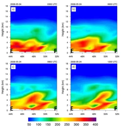
solving convection in global models may not be feasible, but including it in regional studies over areas of deep convection appears crucial.

Profiles of CO vertical mass flux at 09:00 UTC 23 May (Fig. 15) reveal that the con-trasts seen at 500 hPa (Fig. 14) occur throughout the troposphere. The profile was com-puted over the same area (D3) as Fig. 14, but at the time of peak squall line intensity.

5

Although the greatest vertical velocities are in the middle troposphere, the largest CO fluxes are near the surface, due to the much greater CO concentrations in the bound-ary layer. The 5 km simulation produces the greatest upward, downward, and net CO vertical transport at all levels. D1 and D2 again exhibit little difference in their fluxes. Maximum upward fluxes based on D1 and D2 resolution are located somewhat higher

10

in the atmosphere than those from D3 resolution, and their values are approximately an order of magnitude smaller than from D3. All three resolutions produce maximum downward flux in the lower troposphere (∼800 hPa).

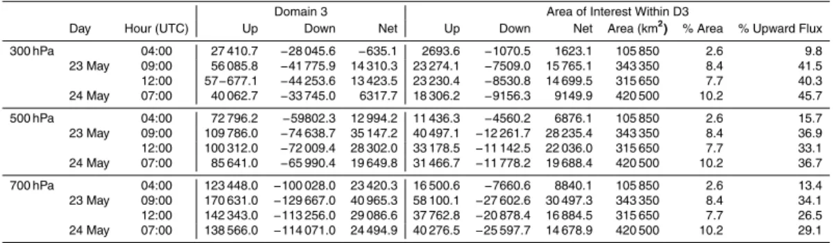
We examined the vertical transport in greater detail between 04:00 UTC 23 May and 07:00 UTC 24 May (Table 2). Each hour we defined an area of interest (AOI) in the 5 km

15

domain (D3, Fig. 4) based on simulated radar reflectivity. There was some subjectivity in defining the AOIs. They encompassed the main convective areas of the squall line each hour, including all regions of updrafts and downdrafts. The northern extent of each AOI was located where the convection began to have a more west-to-east than north-to-south orientation. The southern boundary of each AOI extended to the southern end

20

of the continuous squall line. In the example at 09:00 UTC (Fig. 4b), the convection in the far southern portion of the box was not considered part of the squall line, but within the next 1–2 h, it merged with the convection to the north and was considered part of the line (Fig. 4b–c). Due to these criteria, the sizes of the AOIs vary considerably during the life cycle of the squall line. The area of each AOI is given in Table 2. We also

25

defined an AOI over the multi-cell coastal convection that occurred near 07:00 UTC 24 May (Fig. 4d). We then computed CO vertical fluxes within each AOI.

(23)

ACPD

13, 14871–14925, 2013

cyclone

Title Page

Tables Figures

◭ ◮

Back Close

Full Screen / Esc

Discussion

P

a

per

|

Dis

cussion

P

a

per

|

Discussion

P

a

per

|

Discussio

n

P

a

per

the AOIs. As the squall line begins to form at 04:00 UTC, the area of the AOI is only 2.6 % of the area of the total D3 region. However, the upward transport due to the squall line AOI is 13.4 % of the total at 700 hPa, 15.7 % at 500 hPa, and 9.8 % at 300 hPa. This difference becomes even greater as the squall line develops further. At 09:00 UTC when the squall line is near peak intensity and area coverage, the area of the AOI is

5

approximately 8.4 % of D3, but the transport within the AOI compared to D3’s total is 34.1 % at 700 hPa, 36.9 % at 500 hPa, and 41.5 % at 300 hPa (Table 2). Magnitudes are similar at 12:00 UTC, when the area of the AOI is 7.7 % that of D3.

At the time of multi-cell convection at 07:00 UTC 24 May, the AOI comprises 10.2 % of the total domain (Table 2). However, at 300 hPa, the mass flux of CO is approximately

10

45.7 % the value of the entire domain, the greatest percentage of any altitude or time. Corresponding percentages at 500 and 700 hPa are 36.7 % and 29.1 %, respectively. Even though the convection is weaker than the squall line of the previous day, it still lofts a large amount of CO into the upper troposphere.

5 Summary and conclusions

15

The horizontal and vertical transport of atmospheric pollutants depends greatly on syn-optic scale airstreams such as warm conveyor belts within middle latitude cyclones, mesoscale deep convection that is embedded within them, as well as any deep convec-tion that is located elsewhere. Chemical transport models (CTMs) with a horizontal grid spacing of tens to a few hundred kilometers usually faithfully simulate synoptic-scale

20

meteorological systems. However, they cannot resolve details of convective systems because their relatively coarse grid spacing requires that the convection be parameter-ized at the resolution of the model. As a result, many facets of the convection are not faithfully represented, including the strong mesoscale vertical motions that can rapidly transport surface based pollutants high into the atmosphere. Grid spacing less than

25

(24)

ACPD

13, 14871–14925, 2013

cyclone

Title Page

Tables Figures

◭ ◮

Back Close

Full Screen / Esc

Discussion

P

a

per

|

Dis

cussion

P

a

per

|

Discussion

P

a

per

|

Discussio

n

P

a

per

|

This study used the WRF-Chem CTM to simulate a middle latitude cyclone on 23– 24 May 2008 that contained a typical WCB with an embedded squall line, as well as deep convection located away from the cyclone. Simulations were made over three domains (grid spacings of 45, 15, and 5 km) to examine CO transport at the differing resolutions. The model domains were centered over eastern Asia (Fig. 1), completely

5

encompassing the middle latitude cyclone, its associated frontal systems, and flow patterns aloft. Convective parameterization was used in the outer two domains, while convection was explicitly resolved in the innermost domain.

The simulated middle latitude cyclone began near 12:00 UTC 22 May and lasted several days (Fig. 2a–d). A WCB was located ahead of the surface cold front with

10

an embedded squall line on 23 May, followed by multi-cellular convection on 24 May (Fig. 4). Locations of these simulated features agreed closely with satellite imagery and WWLLN lightning data (Fig. 3), thereby supporting the validity of the simulations. The cyclone’s cold front and associated deep convection passed through an area of surface CO concentrations exceeding 400 ppbv (Fig. 5), producing vertical transport

15

into the free troposphere where horizontal wind speeds are stronger than near the surface.

Forward trajectories based on the WRF-Chem simulations were calculated using the HYSPLIT model. Comparisons were made between the coarse resolution (D1, 45 km) and finer resolution (D3, 5 km) simulations. Trajectories were launched at 06:00 UTC 23

20

May at 500 m above ground and run for 48 h or until they left model domain D1. These trajectories simulated the WCB, with gradual ascent occurring between the surface to 6–7 km altitude (Fig. 6a, c). Trajectories also were launched at a grid spacing of 5 km (domain D3) encompassing the simulated squall line ahead of the cold from. These trajectories vividly revealed the strong convective transport embedded within

25

the WCB. Rapid ascent to heights>_{10 km occurred within 1 h of convective initiation}

(25)

ACPD

13, 14871–14925, 2013

cyclone

Title Page

Tables Figures

◭ ◮

Back Close

Full Screen / Esc

Discussion

P

a

per

|

Dis

cussion

P

a

per

|

Discussion

P

a

per

|

Discussio

n

P

a

per

The WCB at 45 km grid spacing lofted CO values exceeding 275 ppbv from the boundary layer to altitudes of 6–7 km (Fig. 7). The lofted CO plume passed over the cyclone’s warm front and then was transported eastward toward the Pacific Ocean. Conversely, CO transported by the much stronger explicitly resolved convection was rapidly lifted to 10 km. The plume spread horizontally upon reaching the tropopause

5

(Figs. 11–13).

The vertical transport of CO by the squall line on 23 May was much greater than by the multi-cell convection that reformed ahead of the cold front on 24 May. Cross sec-tions of CO parallel and perpendicular to the squall line illustrated the large magnitude of the transport. Along the squall line, CO was transported to altitudes of 10–12 km

10

(Fig. 12a–b). The multi-cell convection along the coast on 24 May (Fig. 12c) lofted CO to 10–12 km, but the areas of upward transport were more isolated, and surface CO concentrations were smaller. Although these weaker and more separated areas of as-cent still transported CO upward and then spread it horizontally, the magnitude of the transport was not as great.

15

An area of deep convection over southeast China, unrelated to the WCB, also lofted CO to altitudes exceeding 10 km (Fig. 10). However, this transport occurred relatively slowly because the convection was located in the coarse domain where it was parame-terized. Transport to the upper troposphere occurred because the convection persisted for 36 h over the same area (Fig. 3), allowing the convective parameterization to

pro-20

duce long lasting but weaker ascent.

CO vertical mass fluxes were computed at several altitudes over the area encom-passed by D3, using WRF-Chem data at each of the three resolutions. Results showed that the simulation at 5 km grid spacing produced substantially greater upward, down-ward, and net CO flux when compared to fluxes based on the output from the coarser

25

D1 and D2 simulations (Fig. 14). Values of upward flux based on the 5 km grid spacing and explicit convection were as large as 50 000t_h−1_{just before convection began and}

exceeded 110 000t_h−1_{during peak intensity of the squall line. Conversely, upward flux}

(26)

ACPD

13, 14871–14925, 2013

cyclone

Title Page

Tables Figures

◭ ◮

Back Close

Full Screen / Esc

Discussion

P

a

per

|

Dis

cussion

P

a

per

|

Discussion

P

a

per

|

Discussio

n

P

a

per

|

There were similar differences in magnitudes for the downward and net fluxes during the periods of convection. During a lull in the convection, magnitudes of net fluxes from the three domains were more similar. These resolution differences were evident at all altitudes examined (Fig. 15). The maximum net flux from the 5 km data occurred at a higher altitude than observed with the D1 or D2 data. However, all three resolutions

5

yielded maximum upward flux near the surface, due to large CO values in the boundary layer.

We further examined the importance of convective transport by defining specific ar-eas of interest (AOIs) within the 5 km domain (Fig. 4). These AOIs encompassed the simulated squall line and the multi-cell storms that formed later. When the squall line

10

was most intense (09:00 UTC 23 May), the area of the AOI comprised only 8.4 % of the total D3 domain, but was responsible for 36.9 % of the vertical transport within the domain at 500 hPa (Table 2). Similar contrasting magnitudes were found at other altitudes and times. During the multi-cellular coastal convection on 24 May, the AOI comprised the greatest percentage of the total domain (10.2 %) and contained 45.7 %

15

of the transport within the domain. Although the convection was multi-cellular, and less intense than the squall line of the previous day, it continuously passed over the same area, lofting large amounts of CO into the atmosphere.

These WRF-Chem simulations reveal major differences in vertical CO transport be-tween parameterized and explicitly resolved convection. Simply decreasing the

reso-20

lution from 45 km to 15 km did not produce major differences in vertical CO transport because parameterization is required at both resolutions. However, the transport was greatly enhanced by increasing the resolution to 5 km which permitted explicit resolu-tion of the convecresolu-tion. Parameterized convecresolu-tion produces weak ascent that is hoped to represent conditions at the coarse resolution of the model. However, this

convec-25

(27)

ACPD

13, 14871–14925, 2013

cyclone

Title Page

Tables Figures

◭ ◮

Back Close

Full Screen / Esc

Discussion

P

a

per

|

Dis

cussion

P

a

per

|

Discussion

P

a

per

|

Discussio

n

P

a

per

Computing requirements may prohibit the use of high resolution simulations with explicit convection over large or global domains. However, limited area, high resolution domains could be embedded within a coarse domain to encompass areas of deep convection (Wang et al., 2004), and they could move with the convection to better simulate the rapid vertical transport that occurs there. Alternatively, one could apply

5

an adaptive mesh refinement (AMR) (e.g., Constantinescu et al., 2008) in which the grid adapts dynamically during the simulation, changing the grid resolution at certain intervals (regriding frequency), with the purpose of controlling the numerical spatial discretization error.

Although our findings are for a single case study, we hypothesize that they are

appli-10

cable to many middle latitude cyclones that contain deep convection, and also to areas of convection not associated with wave cyclones. The results demonstrate the impor-tance of explicitly resolving convection and why it should be used whenever possible. Additional studies must be performed for cyclones and convection of varying strengths and area coverage and in other areas of the globe to better understand convective

15

transport and its influence on atmospheric chemistry.

Acknowledgements. We appreciate the assistance of Steven Peckham in running WRF-Chem. Personnel at Florida State University’s High Performance Computing center assisted in com-piling WRF-Chem and several other programs. Louisa Emmons at NCAR provided the data from MOZART, and Robert Holzworth of the University of Washington provided the WWLLN 20

data. This research was sponsored by the NASA Tropospheric Chemistry Program under Grant NNX0AH72G.

References

Abarca, S. F., Corbosiero, K. L., and Galarneau Jr., T. J.: An evaluation of the Worldwide Light-ning Location Network (WWLLN) using the National LightLight-ning Detection Network (NLDN) as 25