ACPD
11, 26521–26570, 2011Isotopes in winter storm precipitation
S. Pfahl et al.
Title Page
Abstract Introduction
Conclusions References
Tables Figures
◭ ◮
◭ ◮
Back Close
Full Screen / Esc
Printer-friendly Version Interactive Discussion
Discussion
P
a
per
|
Dis
cussion
P
a
per
|
Discussion
P
a
per
|
Discussio
n
P
a
per
|
Atmos. Chem. Phys. Discuss., 11, 26521–26570, 2011 www.atmos-chem-phys-discuss.net/11/26521/2011/ doi:10.5194/acpd-11-26521-2011
© Author(s) 2011. CC Attribution 3.0 License.
Atmospheric Chemistry and Physics Discussions
This discussion paper is/has been under review for the journal Atmospheric Chemistry and Physics (ACP). Please refer to the corresponding final paper in ACP if available.
The isotopic composition of precipitation
from a winter storm – a case study with
the limited-area model COSMO
iso
S. Pfahl1, H. Wernli1, and K. Yoshimura2
1
Institute for Atmospheric and Climate Science, ETH Zurich, 8092 Zurich, Switzerland
2
Atmosphere and Ocean Research Institute, University of Tokyo, Tokyo, Japan
Received: 19 August 2011 – Accepted: 20 September 2011 – Published: 22 September 2011 Correspondence to: S. Pfahl ([email protected])
ACPD
11, 26521–26570, 2011Isotopes in winter storm precipitation
S. Pfahl et al.
Title Page
Abstract Introduction
Conclusions References
Tables Figures
◭ ◮
◭ ◮
Back Close
Full Screen / Esc
Printer-friendly Version Interactive Discussion
Discussion
P
a
per
|
Dis
cussion
P
a
per
|
Discussion
P
a
per
|
Discussio
n
P
a
per
|
Abstract
Stable water isotopes are valuable tracers of the atmospheric water cycle, and poten-tially provide useful information also on weather-related processes. In order to further explore this potential, the water isotopes H182 O and HDO are incorporated into the limited-area model COSMO. In a first case study, the new COSMOiso model is used
5
for simulating a winter storm event in January 1986 over the eastern United States as-sociated with intense frontal precipitation. The modelled isotope ratios in precipitation and water vapour are compared to spatially distributedδ18O observations. COSMOiso very accurately reproduces the statistical distribution ofδ18O in precipitation, and also the synoptic-scale spatial pattern and temporal evolution agree well with the
measure-10
ments. Perpendicular to the front that triggers most of the rainfall during the event, the model simulates a gradient in the isotopic composition of the precipitation, with highδ18O values in the warm air and lower values in the cold sector behind the front. This spatial pattern is created through an interplay of large scale air mass advection, removal of heavy isotopes by precipitation at the front and microphysical interactions
15
between rain drops and water vapour beneath the cloud base. This investigation il-lustrates the usefulness of high resolution, event-based model simulations for under-standing the complex processes that cause synoptic-scale variability of the isotopic composition of atmospheric waters. In future research, this will be particularly bene-ficial in combination with laser spectrometric isotope observations with high temporal
20
resolution.
1 Introduction
Stable water isotopes are useful tracers of processes in the global water cycle and are widely applied for, e.g., hydrological and paleo-climatological studies (Gat, 1996). For instance, isotope data from ice cores can be used as a proxy for reconstructing
25
ACPD
11, 26521–26570, 2011Isotopes in winter storm precipitation
S. Pfahl et al.
Title Page
Abstract Introduction
Conclusions References
Tables Figures
◭ ◮
◭ ◮
Back Close
Full Screen / Esc
Printer-friendly Version Interactive Discussion
Discussion
P
a
per
|
Dis
cussion
P
a
per
|
Discussion
P
a
per
|
Discussio
n
P
a
per
|
time scales, the isotopic composition of atmospheric waters and precipitation is sub-ject to strong variability (e.g., Rindsberger et al., 1990; Wen et al., 2010) and potentially provides valuable information on moisture sources, water transport and cloud micro-physics (Lawrence et al., 1982; Smith, 1992; Gedzelman and Arnold, 1994; Pfahl and Wernli, 2008). However, this potential has not yet been fully explored, mostly owing to
5
the complexity of the involved dynamical and microphysical processes and the sparsity of isotope observations with high temporal resolution. More recently, more such data have become available based on new spectrometric measurement techniques, both from in-situ and remote sensing observations (e.g., Sturm and Knohl, 2010; Wen et al., 2010; Schneider et al., 2010). In order to improve our understanding of the
mecha-10
nisms driving isotope variations in these measurements, but also in other observations on longer time scales, numerical models are commonly applied. The most compre-hensive way of simulating all important processes is to incorporate water isotopes into general circulation models (GCMs) of the atmosphere (e.g., Joussaume et al., 1984; Hoffmann et al., 1998; Yoshimura et al., 2008; Risi et al., 2010b). Global models, due
15
to their relatively coarse spatial resolution, are less well suited for exploring synoptic-scale isotopic variability, associated e.g. with the passage of frontal or convective sys-tems. Therefore, isotope physics have also been implemented in limited-area mod-els. Sturm et al. (2005) incorporated water isotopes into the regional climate model REMO, which was subsequently used for investigations on long, climatological time
20
scales (e.g., Sturm et al., 2007). Smith et al. (2006) and Blossey et al. (2010) used cloud resolving models for simulating idealised tropical circulations, focusing on iso-tope variations in the tropical tropopause layer. Yoshimura et al. (2010) simulated the isotopic content of precipitation from an atmospheric river event at the US west coast with the model IsoRSM and compared the results from this case study to observations
25
ACPD
11, 26521–26570, 2011Isotopes in winter storm precipitation
S. Pfahl et al.
Title Page
Abstract Introduction
Conclusions References
Tables Figures
◭ ◮
◭ ◮
Back Close
Full Screen / Esc
Printer-friendly Version Interactive Discussion
Discussion
P
a
per
|
Dis
cussion
P
a
per
|
Discussion
P
a
per
|
Discussio
n
P
a
per
|
In this study, the stable water isotopes H182 O and HDO are incorporated into the non-hydrostatic COSMO model (Steppeler et al., 2003), a limited-area weather forecast and climate model that is operationally used at several European weather services and thus continuously improved with respect to its numerics and physical parameterisations. In order to test this new isotope-enabled model, hindcast simulations of a winter storm
5
event are performed. Such a setup, in which the regional model is run over a few days, driven by reanalysis data and an isotope GCM, has the advantage that the simulated meteorological and water isotope fields can be directly evaluated by comparing with measurements in an event-based manner (cf. Yoshimura et al., 2010).
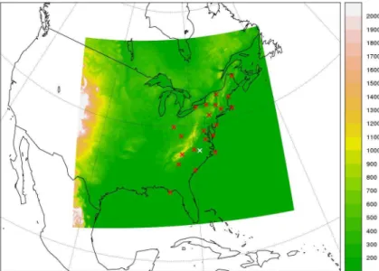
One of the very few cases for which spatially distributed isotope measurements were
10
performed with a high temporal resolution is a winter storm that hit the eastern United States in January 1986. Gedzelman and Lawrence (1990) (in the following referred to as GL90) collected the precipitation at more than 20 stations (see Fig. 1) between 06:00 UTC 18 January 1986 and 06:00 UTC 21 January 1986 with mostly three-hourly, at some stations six-hourly time resolution. Theδ18O content of this precipitation was
15
then analysed in a mass spectrometer. Moreover,δ18O samples were obtained from water vapour at Raleigh-Durham, North Carolina (abbreviated RDU, see again Fig. 1) and from several snow cores from West Virginia (see GL90 for a map of the locations). No analysis of deuterium was performed. GL90 investigated these isotope data using meteorological charts, satellite data and simple, one dimensional model calculations.
20
They found that the height of precipitation formation, the convective or stratiform char-acter of the precipitation and interactions between rain and water vapour beneath the cloud base were important for determining the isotope ratios.
In the present study, on the one hand the data gathered by GL90 are used for evaluat-ing the new regional isotope model. On the other hand, the results from the simulation
25
ACPD
11, 26521–26570, 2011Isotopes in winter storm precipitation
S. Pfahl et al.
Title Page
Abstract Introduction
Conclusions References
Tables Figures
◭ ◮
◭ ◮
Back Close
Full Screen / Esc
Printer-friendly Version Interactive Discussion
Discussion
P
a
per
|
Dis
cussion
P
a
per
|
Discussion
P
a
per
|
Discussio
n
P
a
per
|
mechanisms and, by this, further explore the potential of water isotopes as tracers of weather-related processes.
In Sect. 2, the new regional water isotope model will be introduced and some details on isotope parameterisations will be given. Furthermore, the simulation setup used in this study will be described. In Sect. 3.1 results of the simulation will be presented
5
and compared to observations by GL90. Processes related to isotopic variations in the simulated precipitation will be investigated in more detail in Sect. 3.2. Section 3.3 will then briefly discuss the temperature effect in the model. Finally, Sect. 4 will summarise the most important findings and outline opportunities for future research.
2 Model description
10
2.1 COSMO
The COSMO model (Steppeler et al., 2003) is a non-hydrostatic limited-area model, which is used for operational weather forecasting at several European weather ser-vices, including the German and Swiss weather service. It is based on the primitive fluid-dynamical equations and can be used for simulations with horizontal resolutions
15
of 50 km down to less than one km. The model includes two separate time integra-tion schemes and several different parameterisations for, e.g., cloud microphysics and moist convection. Operationally, the German weather service uses two model setups, the first one with a horizontal grid spacing of 7 km, including a parameterisation of deep convection, and the second one with a grid spacing of 2.8 km and without
parameteris-20
ing deep convection. In addition to short-range forecasts, the COSMO model can also be used for regional climate simulations (e.g., Jacob et al., 2007).
2.2 Water isotope implementation
In order to extend the COSMO model for simulating stable isotopes in the atmospheric water cycle, an approach is adopted similar to previous implementations of isotopes
ACPD
11, 26521–26570, 2011Isotopes in winter storm precipitation
S. Pfahl et al.
Title Page
Abstract Introduction
Conclusions References
Tables Figures
◭ ◮
◭ ◮
Back Close
Full Screen / Esc
Printer-friendly Version Interactive Discussion
Discussion
P
a
per
|
Dis
cussion
P
a
per
|
Discussion
P
a
per
|
Discussio
n
P
a
per
|
in GCMs and regional models (see again Joussaume et al., 1984; Sturm et al., 2005; Blossey et al., 2010, for examples). A parallel water cycle is introduced that does not affect other model components and is used as a purely diagnostic tool. All prognostic moisture fields, which are simulated by the model in terms of specific humidities, are duplicated twice, representing the specific humidities of H182 O and HDO, respectively.
5
From these prognostic specific humidity fields, the isotope ratios in usualδ-notation can be calculated. The implementation is made for a one-moment microphysical scheme with 5 species, namely water vapour, cloud water, cloud ice, rain and snow (for details, see Doms et al., 2005), leading to 10 additional prognostic variables for the heavy isotopes. These additional moisture fields are affected by the same physical processes
10
as the original humidity, e.g., they are transported by large scale winds and are involved in the formation of clouds and precipitation. Only during phase transitions, they behave differently than the standard light water owing to isotopic fractionation. In the following subsections, some details on the transport and microphysical parameterisations of the heavy isotopes will be given.
15
2.2.1 Transport
There are three major mechanisms in the COSMO model that transport moisture in space: moist convection (which will be treated in Sect. 2.2.4), grid-scale advection and boundary layer turbulence. The latter only affects the vertical transport of water vapour and non-precipitating hydrometeors, i.e., turbulent transport is neglected for rain and
20
snow. For the heavy isotopes, the same flux-gradient parameterisation and the same exchange coefficients as for the light water are used. In this way, all isotopes are transported independently of each other.
For the three-dimensional advection of moisture quantities, the Bott advection scheme (Bott, 1989) with fourth order accuracy is applied in our setup. This scheme is
25
positive definite and mass-conserving1. For the advection of different isotope species it
1
ACPD
11, 26521–26570, 2011Isotopes in winter storm precipitation
S. Pfahl et al.
Title Page
Abstract Introduction
Conclusions References
Tables Figures
◭ ◮
◭ ◮
Back Close
Full Screen / Esc
Printer-friendly Version Interactive Discussion
Discussion
P
a
per
|
Dis
cussion
P
a
per
|
Discussion
P
a
per
|
Discussio
n
P
a
per
|
is most important that no fractionation occurs, i.e., that the ratios between two isotopes do not change during adiabatic and frictionless advection. This cannot be guaranteed if the isotope humidities (or, more generally, two arbitrary tracers) are transported in-dependently of each other (Sch ¨ar and Smolarkiewicz, 1996; Risi et al., 2010b), mostly owing to numerical errors and non-linearities in the advection scheme. Therefore, for
5
the transport of heavy isotopes a modified scheme is implemented that employs iso-tope ratios, instead of specific humidities, for estimating the advective fluxes, similar to the approach of Risi et al. (2010b). Details of this scheme and a one-dimensional test are described in Appendix A.
2.2.2 Surface fluxes
10
Surface fluxes of heavy isotopes over the ocean are parameterised using a Craig-Gordon type model (Craig and Craig-Gordon, 1965). Two options for the non-equilibrium fractionation factor are implemented: The first one, which is commonly applied in many isotope models, parameterises the fractionation factor as a function of wind velocity, following Merlivat and Jouzel (1979). The second one uses a wind-speed independent
15
formulation based on the empirical results of Pfahl and Wernli (2009). The second option is chosen for the reference simulation in the present study. To test the impact of this choice, a simulation using the parameterisation by Merlivat and Jouzel (1979) is also performed. Since the simulatedδ18O fields from this experiment are very similar to the results of the reference simulation, they will not be shown in detail in the following.
20
In order to evaluate the difference between the two parameterisations, observations of deuterium excess would be required, which are not available for the storm investigated here. For the isotopic composition of the ocean, a constant, slightly enriched value of
δ18O=1 ‰ is used, roughly corresponding to average surface waters in the western North Atlantic (LeGrande and Schmidt, 2006). Evapotranspiration from land surfaces is
25
ACPD
11, 26521–26570, 2011Isotopes in winter storm precipitation
S. Pfahl et al.
Title Page
Abstract Introduction
Conclusions References
Tables Figures
◭ ◮
◭ ◮
Back Close
Full Screen / Esc
Printer-friendly Version Interactive Discussion
Discussion
P
a
per
|
Dis
cussion
P
a
per
|
Discussion
P
a
per
|
Discussio
n
P
a
per
|
assumed not to fractionate, similar to most isotope models (e.g., Hoffmann et al., 1998; Yoshimura et al., 2008; Risi et al., 2010b). In future work, water isotopes will also be incorporated into the land surface scheme of the COSMO model, involving a more complete parameterisation of isotope fluxes from land surfaces. Nevertheless, for the present case study these land surface processes are not assumed to be crucial. The
5
isotopic composition of the soil water is adopted from the IsoGSM model (Yoshimura et al., 2008, see also Sect. 2.2.5).
2.2.3 Cloud microphysics
In the microphysical scheme, transfer rates between the different water species during the formation of clouds and precipitation are specified. For example, the transfer rate
10
Sau of cloud waterqc to form rain qr by autoconversion is then part of the tendency equations of the specific humidities:
∂qc
∂t =...−Sau+...
∂qr
∂t =...+Sau+...
(1)
Since a one-moment scheme is used, specific humidities are the only prognostic vari-ables, and information about the sizes of the different particles is only implicitly taken
15
into account. The isotopic composition of the particles is assumed to be independent of their size. For all microphysical interactions that do not involve the vapour phase (e.g., autoconversion of cloud particles to form rain or freezing of liquid water), there is no isotopic fractionation, and the transfer rateshS of the heavy isotopes, following Blossey et al. (2010), are given by
20
hS =
hq s lq
s
ACPD
11, 26521–26570, 2011Isotopes in winter storm precipitation
S. Pfahl et al.
Title Page
Abstract Introduction
Conclusions References
Tables Figures
◭ ◮
◭ ◮
Back Close
Full Screen / Esc
Printer-friendly Version Interactive Discussion
Discussion
P
a
per
|
Dis
cussion
P
a
per
|
Discussion
P
a
per
|
Discussio
n
P
a
per
|
wherehqs andlqs are the specific humidities of heavy and light isotopes, respectively, in the source phase andlS is the transfer rate of the standard light isotope2.
During phase transitions involving water vapour, isotopic fractionation occurs. For its parameterisation, equilibrium fractionation factorsαe with respect to liquid water and
ice are calculated following Majoube (1971) and Merlivat and Nief (1967), respectively.
5
Here, these fractionation factors are defined to give the ratio between the isotopic com-position of vapour and the condensed phase, i.e., they are smaller than 1. Molecular diffusivities from measurements by Merlivat (1978) are applied. In the COSMO model, condensation and evaporation of cloud water are parameterised with the help of a satu-ration adjustment technique, implying thermodynamic equilibrium between vapour and
10
liquid clouds. Also for the heavy isotopes, an equilibrium approach can be adopted, since the equilibration time with respect to small droplets typically is in the order of seconds (see again Blossey et al., 2010). This leads to a diagnostic equation for the isotope ratio in cloud water, as given by Blossey et al. (2010) in their Eq. (B21).
For rain drops, owing to their larger size, the assumption of isotopic equilibrium is
15
not valid, and the mass transfer between the drop and the surrounding vapour has to be modelled in an explicit way. This affects the total moisture budget of the drop only beneath the cloud base, where the rain falls into unsaturated air and starts evaporat-ing. The isotopic content of the rain, however, may also change within the cloud. In COSMO, the transfer rate due to rain evaporation is parameterised by
20
lS
ev=F(lqr)
q⋆l −lqv, (3)
whereql⋆denotes the saturation humidity with respect to liquid water, andqvandqrare
the specific humidities of water vapour and rain, respectively. The functionF depends, in addition to the rain content qr, also on water diffusivity. However, in COSMO this
2
ACPD
11, 26521–26570, 2011Isotopes in winter storm precipitation
S. Pfahl et al.
Title Page
Abstract Introduction
Conclusions References
Tables Figures
◭ ◮
◭ ◮
Back Close
Full Screen / Esc
Printer-friendly Version Interactive Discussion
Discussion
P
a
per
|
Dis
cussion
P
a
per
|
Discussion
P
a
per
|
Discussio
n
P
a
per
|
dependence is not explicitly taken into account, but rather included in a semi-empirical constant. Because of this, the heavy isotopes are not implemented directly via their diffusivities here (this would imply a change also in the standard transfer rate), but a semi-empirical approach is used based on a study by Steward (1975). In future research, it may be tested how this implementation compares with a more theoretical
5
strategy as employed, e.g., by Blossey et al. (2010). Following Steward (1975), the heavy isotope mass exchange ratedhm/dtbetween a rain drop and the surrounding vapour is related to the total mass exchange ratedlm/dtby
dhm
dt =
dlm
dt h
D
lD
!n
αeq⋆l hqr/lqr−hqv ql⋆−lq
v
. (4)
The rightmost fraction contains the humidity gradients of heavy (numerator) and light
10
(denominator) isotopes between drop surface and the surrounding vapour. hD andlD
are the diffusivities of heavy and light isotopes, respectively. Based on the measure-ments by Steward (1975), the exponent n is chosen to be 0.58, independent of the drop size (see also Bony et al., 2008). Combining Eqs. (3) and (4), one obtains the heavy isotope transfer rate for rain evaporation and equilibration with the surrounding
15
vapour:
hS
eveq=F(lqr) hD
lD
!n
αeq⋆l
h
qr
lq r
−hqv
!
. (5)
In the case of rain falling through clouds, there is no evaporation and the transfer rate
l
Sev specified in Eq. (3) vanishes. Nevertheless, Eq. (5) shows that there may be a non-vanishing transfer of heavy isotopes also in this case if rain and vapour are not in
20
isotopic equilibrium.
ACPD
11, 26521–26570, 2011Isotopes in winter storm precipitation
S. Pfahl et al.
Title Page
Abstract Introduction
Conclusions References
Tables Figures
◭ ◮
◭ ◮
Back Close
Full Screen / Esc
Printer-friendly Version Interactive Discussion
Discussion
P
a
per
|
Dis
cussion
P
a
per
|
Discussion
P
a
per
|
Discussio
n
P
a
per
|
the ice particles. During deposition, the water vapour interacts only with the outermost layer of the particles, whose isotopic composition is assumed to be equal to the isotopic composition of the deposition flux. In addition to equilibrium fractionation, kinetic effects occur if the air is super-saturated with respect to ice. This is parameterised using a combined fractionation factor given by Jouzel and Merlivat (1984) in their Eq. (14)
5
(which is equivalent to Eq. (B26) of Blossey et al., 2010). The ratio of the ventilation factors of light and heavy isotopes,lf /hf, which is needed in this equation, is set to 1 for deposition on small ice crystals and to 0.995 for deposition on snow flakes. The latter is a typical value for particles between 0.5 and 1 mm in length (see again Jouzel and Merlivat, 1984). An advantage of the COSMO microphysical scheme compared to
10
other models is that the supersaturation is predicted in a prognostic way. No saturation adjustment is used over ice (in contrast, e.g., to the model of Blossey et al., 2010), and there is no need for prescribing supersaturation as a function of temperature (cf. Jouzel and Merlivat, 1984; Hoffmann et al., 1998; Risi et al., 2010b). The sublimation of ice and snow particles is assumed to occur without isotopic fractionation, and since
15
no information is available about the layering of single particles, the average isotope composition of ice or snow is used for the sublimation flux (see again Bony et al., 2008; Blossey et al., 2010).
2.2.4 Moist convection
For the parameterisation of moist convection, a modified version of the Tiedtke mass
20
flux scheme (Tiedtke, 1989) is applied in the COSMO model (see again Doms et al., 2005, for details). In order to implement heavy isotopes in this parameterisation, the humidity variables are duplicated, as described above. All physical processes during simulated convective up- and downdraft affect the heavy isotopes in a similar way as the standard light humidity. Also the closure assumptions, e.g., the entrainment and
25
ACPD
11, 26521–26570, 2011Isotopes in winter storm precipitation
S. Pfahl et al.
Title Page
Abstract Introduction
Conclusions References
Tables Figures
◭ ◮
◭ ◮
Back Close
Full Screen / Esc
Printer-friendly Version Interactive Discussion
Discussion
P
a
per
|
Dis
cussion
P
a
per
|
Discussion
P
a
per
|
Discussio
n
P
a
per
|
the former, isotope fractionation is parameterised using an equilibrium approach, as described in Sect. 2.2.3. With respect to ice, kinetic fractionation is taken into account following Jouzel and Merlivat (1984). Here, the supersaturation is prescribed as a func-tion of temperature, with the tuning parameterλset to 0.004 (Risi et al., 2010b). In a temperature range between−23 ◦C and 0◦C, clouds are supposed to consist of both
5
liquid and ice particles, and the isotopic composition of the condensate is interpolated between the two phases, assuming a quadratic increase of the liquid water fraction with temperature (note that in this case, the diagnostic relationship for the isotopic compo-sition of cloud water is replaced by a closed system approach, similar to Bony et al., 2008).
10
In the Tiedtke scheme, saturation in the convective downdrafts is assumed to be maintained by evaporation of falling precipitation. The isotopic composition of the evap-orate from liquid precipitation is calculated using a closed model with isotopic equilib-rium (since the relative humidity is always 100%). Beneath the cloud base, in unsatu-rated conditions, the evaporation rate of rain is parameterised following Kessler (1969).
15
For the heavy isotopes, this liquid evaporation rate is scaled according to Eq. (4), again incorporating kinetic effects based on measurements by Steward (1975). No fractiona-tion occurs during the sublimafractiona-tion of solid precipitafractiona-tion (see again Sect. 2.2.3), and in the mixed phase range interpolation is used. The isotopic composition of the precip-itation is obtained from the vertically integrated precipprecip-itation fluxes, as no prognostic
20
information on the rain or snow water content on a specific level is available in the scheme.
2.2.5 Initial and boundary data
Since COSMO is a regional model, boundary data have to be provided for all prognostic variables. In this study, ERA40 reanalyses (Uppala et al., 2005) from the European
25
ACPD
11, 26521–26570, 2011Isotopes in winter storm precipitation
S. Pfahl et al.
Title Page
Abstract Introduction
Conclusions References
Tables Figures
◭ ◮
◭ ◮
Back Close
Full Screen / Esc
Printer-friendly Version Interactive Discussion
Discussion
P
a
per
|
Dis
cussion
P
a
per
|
Discussion
P
a
per
|
Discussio
n
P
a
per
|
the COSMO grid (see Sect. 2.3). After the model initialisation, information from the ERA40 data is only used at and close to the model boundaries, employing a relaxation scheme following Davies (1976). No nudging of the COSMO fields is performed in the interior of the model domain. For the water isotopes, initial and boundary data are taken from a historical isotope GCM simulation by Yoshimura et al. (2008), who
5
employed the IsoGSM global model with the atmospheric circulation constrained to reanalysis data with the help of a nudging technique. Isotope data from other GCM simulations could also be applied in future research. Isotope ratios in water vapour with a spectral resolution of T62 and on 17 vertical levels are obtained from the IsoGSM simulations. The isotope data are transferred to the COSMO model grid in the same
10
way as the ERA40 humidity fields using linear interpolation. Since IsoGSM does not simulate hydrometeors in a prognostic way, boundary data for isotope ratios in cloud water and ice are calculated from the isotope ratios in vapour by assuming isotopic equilibrium with respect to liquid water and ice, respectively. The boundary relaxation of the water isotope data is done based on isotope ratios instead of specific humidities,
15
since this leads to more stable results. For the three-dimensional rain and snow fields, no boundary data are provided by ERA40. A no-flux boundary condition is used for these variables and the corresponding heavy isotopes.
2.3 Simulation setup
In the following, the COSMO model with the water isotope implementation will be
20
named COSMOiso. In this study, the new model, based on COSMO version 4.11, is applied for hindcast simulations with an integration time of 126 h. A horizontal grid spacing of 0.0625◦(in a rotated grid), corresponding to approximately 7 km, and 40 hy-brid vertical levels are used. For the time integration, a third order Runge-Kutta scheme is applied. The model domain covers the eastern United States, parts of Canada and
25
ACPD
11, 26521–26570, 2011Isotopes in winter storm precipitation
S. Pfahl et al.
Title Page
Abstract Introduction
Conclusions References
Tables Figures
◭ ◮
◭ ◮
Back Close
Full Screen / Esc
Printer-friendly Version Interactive Discussion
Discussion
P
a
per
|
Dis
cussion
P
a
per
|
Discussion
P
a
per
|
Discussio
n
P
a
per
|
days of the model integration. During this time, a winter storm developed over the east-ern US and theδ18O content of the precipitation at several stations was measured by GL90 (see Sect. 1).
In addition to the reference simulation with isotope physics parameterised as de-scribed in Sect. 2.2, a sensitivity experiment is performed. In this experiment, isotope
5
fractionation during the interaction of rain and water vapour is switched of, such that no equilibration of the falling rain droplets occurs and the isotope ratio of the vapour evaporating from rain drops is equal to the composition of the rain. In the next section, results from the reference simulation and this sensitivity experiment will be presented.
3 Results and discussion
10
3.1 Model evaluation
3.1.1 Meteorology
In order to be able to reasonably simulate isotopic variations in atmospheric waters in comparison with event-based observations, first of all the meteorological conditions simulated by COSMOiso should be realistic. For the winter storm event modelled here,
15
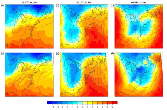
this is checked by comparing COSMOiso results with ERA40 reanalyses. Figure 2 shows the temperature on 850 hPa and the sea level pressure (SLP) from both model and reanalysis at 00:00 UTC on the last three days of the simulation period. A region covering the central part of the model domain is shown, which will be the same for all horizontal maps in the following. At 00:00 UTC 19 January (Fig. 2a), the temperature
20
structure over the US and the western North Atlantic is relatively zonal. Only in the north-west of the displayed region, south of the Great Lakes, colder air masses spread southward, coinciding with a shallow, meridionally extended low pressure anomaly. During the following day, this colder air moves in south-easterly direction, the horizontal temperature gradient becomes more pronounced, and the low pressure system slightly
ACPD
11, 26521–26570, 2011Isotopes in winter storm precipitation
S. Pfahl et al.
Title Page
Abstract Introduction
Conclusions References
Tables Figures
◭ ◮
◭ ◮
Back Close
Full Screen / Esc
Printer-friendly Version Interactive Discussion
Discussion
P
a
per
|
Dis
cussion
P
a
per
|
Discussion
P
a
per
|
Discussio
n
P
a
per
|
intensifies. At 00:00 UTC 20 January (Fig. 2b), it is located over the US east coast, and an elongated front separates the cold air masses over the interior of the continent from the warmer coastal and maritime air. Subsequently, the low pressure system moves north-eastwards and further intensified, reaching central pressure values below 992 hPa. At 00 UTC on the following day, its centre reaches New England and the
5
Canadian border (Fig. 2c). The cold sector of the cyclone at this date covers the north-east of the United States and parts of the western North Atlantic. This synoptic evolution is properly represented by COSMOiso (Fig. 2d–f). The most pronounced differences to the ERA40 data occur after 5 days of the simulation (cf. Fig. 2c,f), when the low pressure anomaly simulated by COSMOiso is stronger than in the reanalysis
10
data. This may be partly due to the much finer spatial resolution. Furthermore, the temperature close to the cyclone centre is underestimated by the model. Apart from this, temperature and SLP differences between the two datasets are mostly minor and restricted to regional scales.
In Figure 3, geopotential height on 500 hPa and precipitation from ERA40 and
15
COSMOiso are shown. Note that the dates differ from those in Fig. 2; here, data at 12:00 UTC 19 January, 00:00 UTC 20 January and 12:00 UTC 20 January are dis-played. Precipitation is accumulated over a six-hourly period comprising the respective dates. The ERA40 precipitation has been obtained from short-term forecasts of the ECMWF model, considering forecast steps from 9 to 15 h. The geopotential height
20
contours in Fig. 3 show a pronounced upper level trough moving in easterly direction, which induces the advection of cold air described above. The formation and intensifi-cation of a cutoffto the west of the surface low is less pronounced in the COSMOiso simulation compared to the ERA40 data. Both the ECMWF model and COSMOiso sim-ulate precipitation over the continent mostly along the cold front of the cylcone and in
25
ACPD
11, 26521–26570, 2011Isotopes in winter storm precipitation
S. Pfahl et al.
Title Page
Abstract Introduction
Conclusions References
Tables Figures
◭ ◮
◭ ◮
Back Close
Full Screen / Esc
Printer-friendly Version Interactive Discussion
Discussion
P
a
per
|
Dis
cussion
P
a
per
|
Discussion
P
a
per
|
Discussio
n
P
a
per
|
more rainfall in the warm sector, especially at 12:00 UTC 19 January. Of course, the spatial variability in the COSMOisofields is much larger, owing to the smaller grid spac-ing. Nevertheless, most of the continental precipitation in COSMOiso is of large-scale character, only in the southern parts close to the coast there are some contributions from the convection scheme. Hence, the influence of this scheme (whose
microphys-5
ical parameterisations are relatively simple, cf. Sect. 2.2.4) on the results is small. In addition, both models simulate a band of more convective precipitation over the ocean (see again Fig. 3), partly associated with the cold front of the cyclone, which will not be investigated in detail here, since no isotope data from this oceanic region are available. All together, Figs. 2 and 3 show that the meteorological conditions during the winter
10
storm in January 1986 are adequately simulated by COSMOiso. In particular, the mod-elled evolution of the temperature field, dominated by the passage of a large frontal system, and the track of the associated cyclone agree well with the ERA40 reanalysis data. With respect to precipitation, differences between the models are larger, also re-lated to the huge impact of the horizontal resolution on the simure-lated spatial structures.
15
When comparing isotope data from COSMOiso with station observations, it should be kept in mind that there is some uncertainty related to the exact timing and intensity of the modelled precipitation at a specific location.
3.1.2 Water isotopes
For evaluating the new COSMOiso model, first the isotope ratios in precipitation from
20
the reference simulation are compared to observations by GL90 using statistical means. Probability density functions (PDFs) of δ18O in precipitation are fitted from both model data (for the analysis period 06:00 UTC 18 January to 06:00 UTC 21 Jan-uary, cf. Sect. 2.3) and measurements using a non-parametric method with Gaussian kernels. Isotope data are not weighted with precipitation intensity, and all three- and
25
ACPD
11, 26521–26570, 2011Isotopes in winter storm precipitation
S. Pfahl et al.
Title Page
Abstract Introduction
Conclusions References
Tables Figures
◭ ◮
◭ ◮
Back Close
Full Screen / Esc
Printer-friendly Version Interactive Discussion
Discussion
P
a
per
|
Dis
cussion
P
a
per
|
Discussion
P
a
per
|
Discussio
n
P
a
per
|
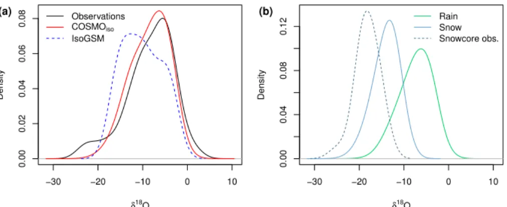
again Fig. 1), taking into account that there is little to no precipitation in the western part of the model domain. The PDFs ofδ18O in total precipitation are shown in Fig. 4a. There is a very good agreement between the COSMOisoresults and the observations. Both PDFs have a maximum close to −6 ‰. The medians of the δ18O distributions from measurement and model data are−7.4 ‰ and−7.9 ‰, respectively, and their
in-5
terquartile ranges are 6.4 ‰ and 6.5 ‰. Only for very low and very highδ18O values, there are some differences between the PDFs. These deviations at the tails of the distributions, which are governed by isotope ratios in snow and very weak rain, might be related to insufficient observational sampling. The PDF from COSMOiso is almost identical if six-hourly instead of three-hourly data are used, indicating that differences
10
in the sampling time hardly influence the results. For comparison, Fig. 4a also shows a PDF ofδ18O in precipitation from IsoGSM, the global model that is used for initialising the isotope ratios in water vapour (see Sect. 2.2.5). Since the large scale circulation of IsoGSM is nudged to reanalysis data (see again Yoshimura et al., 2008), the model, in spite of its coarse spatial resolution, reproduces the large scale features of the frontal
15
precipitation reasonably well (not shown). The PDF of δ18O is fitted based on six-hourly output of precipitation rates, using land data from the same latitude range as for COSMOiso and between 105◦W and 60◦W longitude. As can be seen from the figure,
δ18O values from IsoGSM are in the same range as the observations, but the distri-bution is shifted to lower isotope ratios. The median of the IsoGSM data is−10.4 ‰,
20
and the interquartile range is 7.7 ‰. In Fig. 4b, PDFs ofδ18O in rain and snow from COSMOisoare displayed separately. There is a clear separation between higher values for rain, which constitutes the major part of the precipitation, and lower isotope ratios in snow. Unfortunately, no information on the phase of the precipitation is available from the station observations. Therefore, a PDF is only shown for the snowcore data
gath-25
ACPD
11, 26521–26570, 2011Isotopes in winter storm precipitation
S. Pfahl et al.
Title Page
Abstract Introduction
Conclusions References
Tables Figures
◭ ◮
◭ ◮
Back Close
Full Screen / Esc
Printer-friendly Version Interactive Discussion
Discussion
P
a
per
|
Dis
cussion
P
a
per
|
Discussion
P
a
per
|
Discussio
n
P
a
per
|
These results show that COSMOiso very accurately reproduces the statistical distri-bution ofδ18O in precipitation during the winter storm in January 1986. Compared to a global model with lower spatial resolution, the more detailed representation of the synoptic processes leads to an improvement of theseδ18O statistics. In the following, the spatial and temporal patterns of the water isotopes are compared to the station
5
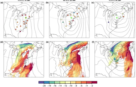
data. Figure 5 showsδ18O in six-hourly precipitation from observations by GL90 and the COSMOiso reference simulation for the three dates previously displayed in Fig. 3. Model data are only shown where the six-hourly precipitation exceeds 0.6 mm. Grey contours indicate the SLP from ERA40 and COSMOiso. At 12:00 UTC 19 January (Fig. 5a, d), δ18O ratios from both observations and model simulation are relatively
10
high, in particular in a band reaching from the south-westerly edge of the precipitation region to the north-east. Lower values were observed at the westernmost station, in agreement with the model. At the two stations south of Lake Ontario, very high isotope ratios were measured. COSMOiso does not simulate any precipitation at the locations of these stations, but also highδ18O at the western shore of the lake. The agreement
15
between model and observations is worse at the south-easterly coastal stations, where modelled precipitation rates are very heterogeneous. The lowestδ18O ratios are simu-lated in the very north, where solid precipitation reaches the ground, as indicated by the red dashed line marking the transition between rain and snow. The overall consistency between COSMOiso and the isotope observations is worse at 00:00 UTC 20 January
20
(Fig. 5b ,e), in particular at the stations close to the Canadian border, where measured values are quite variable and do not resemble the spatial gradient simulated by the model. At the more southerly stations, there is again a better agreement, with higher values at the coast and lower values further inland. COSMOiso does not simulate pre-cipitation as far west as it was observed (in contrast to the ECMWF model, see again
25
ACPD
11, 26521–26570, 2011Isotopes in winter storm precipitation
S. Pfahl et al.
Title Page
Abstract Introduction
Conclusions References
Tables Figures
◭ ◮
◭ ◮
Back Close
Full Screen / Esc
Printer-friendly Version Interactive Discussion
Discussion
P
a
per
|
Dis
cussion
P
a
per
|
Discussion
P
a
per
|
Discussio
n
P
a
per
|
stations, but very good further south. As 12 h earlier, very low values were observed at the station in the west, which lies in the same area as the snowcores (see again GL90) that corroborate the lowδ18O ratios in this region. COSMOisodoes not simulate precipitation there, but also an area of very depleted snow at the southwesterly edge of the main precipitation band.
5
In summary, Fig. 5 shows that the large scale spatial patterns of δ18O in precip-itation from the COSMOiso simulation are consistent with observations by GL90. In particular, there is a spatial gradient with highδ18O values at the eastern flank of the main precipitation band and lower values further west. The lowest isotope ratios are modelled and observed in the cold air, where snow reaches the surface. Furthermore,
10
the temporal evolution observed at most of the stations, with high isotope ratios when precipitation starts and more depleted values later in time, is properly reproduced by the model. However, there are also deviations between COSMOisoresults and isotope observations, mostly on regional and local scales. This can be shown more explicitely by comparing time series at specific stations. As an example, the temporal evolution
15
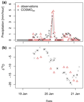
of precipitation and its isotopic composition at the station Avoca, Pennsylvania (AVP; green outer circle in Fig. 5a–c) is displayed in Fig. 6. During the 19th of January, there was only little rainfall at this station3. The main precipitation band passed AVP shortly after 00:00 UTC 20 January, followed by some hours without rain and several smaller showers on late 20 and early 21. This precipitation time series is properly reproduced
20
by COSMOiso. Only before the passage of the main front, some rain is simulated that was not observed at the station. The isotope ratios in precipitation from both model and measurements are relatively high during the 19th and decrease on the 20th of January (Fig. 6b). The model overestimates theδ18O in the beginning and during the precipitation maximum and does not capture the slight increase that was observed at
25
the onset of the showers on the 20th. One reason for this mismatch may be the strong spatial variability of the isotope ratio in precipitation (see again Fig. 5). Due to this,
3
ACPD
11, 26521–26570, 2011Isotopes in winter storm precipitation
S. Pfahl et al.
Title Page
Abstract Introduction
Conclusions References
Tables Figures
◭ ◮
◭ ◮
Back Close
Full Screen / Esc
Printer-friendly Version Interactive Discussion
Discussion
P
a
per
|
Dis
cussion
P
a
per
|
Discussion
P
a
per
|
Discussio
n
P
a
per
|
even small errors in the simulation of the spatial structure of the precipitation field may have a large impact on theδ18O time series at a specific location. Furthermore, GL90 showed that several mesoscale cloud bands influenced the showers at station AVP during the 20th of January. Such mesoscale structures are more difficult to simulate than the large scale synoptic evolution.
5
In contrast toδ18O of precipitation, GL90 sampled the isotopic composition of water vapour only at one location, the station RDU in North Carolina (white cross in Fig. 1). Figure 7 shows the observed and modelled time series at this station. Isotope ratios were in the order of −15 ‰ during the 19th and suddenly dropped to below −23 ‰ around 00:00 UTC 20 January. COSMOisocaptures these values and also the timing of
10
the drop very well. The modelled temperature, which is also shown in Fig. 7, indicates that the decrease in the isotope ratio is related to the passage of the front. Only during the late 20th, there is a discrepancy between the observed and simulated time series, which might again be due to problems with modelling the exact location of the strong spatial gradients ofδ18O in water vapour, discussed further in Sect. 3.2.
15
The results from this section show that for the winter storm event investigated here, COSMOiso is able to simulate the synoptic-scale variability of δ18O in atmospheric waters in good agreement with observations. Based on this, the model can be applied for investigating the physical processes causing such variability. This will be the focus of the next section. Nevertheless, it has to be kept in mind that the model cannot
20
exactly reproduce mesoscale structures and local variations. Therefore, care has to be taken when interpreting time series of the isotopic composition at single locations.
3.2 Processes determining isotope ratios in frontal precipitation
Most of the continental precipitation during the winter storm in January 1986 fell in the region of the evolving cyclonic system crossing the eastern US between 19 and 21
Jan-25
ACPD
11, 26521–26570, 2011Isotopes in winter storm precipitation
S. Pfahl et al.
Title Page
Abstract Introduction
Conclusions References
Tables Figures
◭ ◮
◭ ◮
Back Close
Full Screen / Esc
Printer-friendly Version Interactive Discussion
Discussion
P
a
per
|
Dis
cussion
P
a
per
|
Discussion
P
a
per
|
Discussio
n
P
a
per
|
storm events are rare, owing to the lack of spatially distributed isotope observations and model studies on synoptic scales (cf. Sect. 1). The spatial east-west gradient is connected to a temporal evolution with high δ18O values in the beginning and a de-crease later on at stations where the front passes by (cf. Fig. 6). Such a dede-crease was observed in previous studies on mid-latitude weather systems, e.g., by Rindsberger
5
et al. (1990), Celle-Jeanton et al. (2004) and Coplen et al. (2008)4. The spatial gradi-ent and corresponding time evolution thus appear to be rather typical for mid-latitude frontal systems. Understanding the processes driving this isotopic gradient is the focus of the present section.
One advantage of a model-based investigation of synoptic-scale isotope
variabil-10
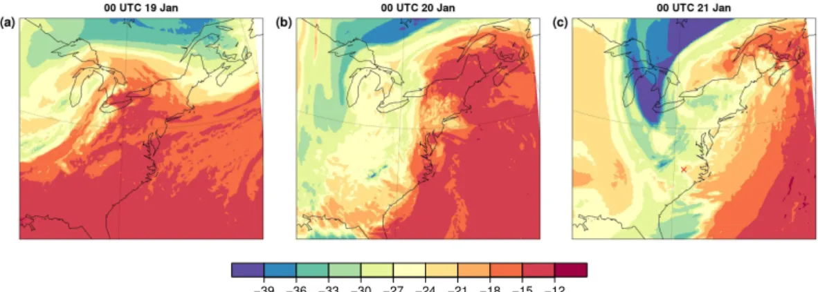
ity, compared to discrete observations at specific stations, is the complete spatial and temporal coverage, which can provide additional insights into the relationship between meteorological and isotopic fields. Figure 8 shows the spatial distribution ofδ18O in water vapour approximately 1 km above the surface at 00:00 UTC on 19, 20 and 21 January. There is a relatively close correspondence between these fields and the
15
temperature on 850 hPa plotted in Fig. 2. Isotope ratios are rather high in the warm, pre-frontal air and lower in the cold air mass that has been transported into the domain from the north-west. This distribution points towards a large-scale control of the diff er-ent air masses on theδ18O gradient in precipitation along the front. In the pre-frontal air, clouds and precipitation form from (and equilibrate with) enriched water vapour,
20
and thusδ18O in precipitation also is relatively high. Behind the front, more depleted water vapour leads to lowerδ18O in precipitation. This process is strongly related to the classical temperature effect (Dansgaard, 1964), which provides the basis for water isotope paleo-thermometry. Water vapour in colder air further poleward has, on aver-age, been exposed to more condensation and removal of heavy isotopes than warmer
25
(and in the present case also more oceanic) air in the south, leading to a climatological decrease ofδ18O in vapour (and thereby precipitation) with temperature. This effect is
4
ACPD
11, 26521–26570, 2011Isotopes in winter storm precipitation
S. Pfahl et al.
Title Page
Abstract Introduction
Conclusions References
Tables Figures
◭ ◮
◭ ◮
Back Close
Full Screen / Esc
Printer-friendly Version Interactive Discussion
Discussion
P
a
per
|
Dis
cussion
P
a
per
|
Discussion
P
a
per
|
Discussio
n
P
a
per
|
mainly imprinted on the COSMOiso vapour field by the initial and boundary conditions. However, the large scale relationship betweenδ18O in vapour and frontal precipitation observed here is not only due to a climatological pre-conditioning of the vapour, but there is also a contribution by the weather system itself, which induces gradual rainout and isotopic depletion of the vapour along the front.
5
In addition to the climatological decline of δ18O in water vapour with decreasing temperature in the horizontal, there is also a decrease with altitude, owing to the pro-gressive removal of heavy isotopes when air rises and cools. GL90, using cloud top temperature observations from satellites, argued that because of this vertical gradient the altitude of precipitation formation influenced the isotopic composition of surface
10
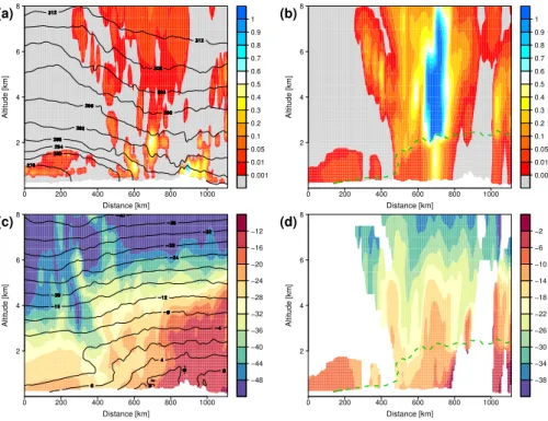
precipitation during the 1986 storm. In order to investigate if this effect contributed sys-tematically to the horizontal gradient inδ18O in precipitation perpendicular to the front, a vertical cross section along the dashed green line in Fig. 3d at 12:00 UTC 19 January is shown in Fig. 9. In addition to the specific moisture content of non-precipitating and precipitating hydrometeors, the Figure shows the isotopic composition of water vapour
15
as well as rain and snow. The simulated surface cold front at this instant is located in a distance of approximately 600 km from the westernmost point of the cross section, as indicated by the isentropes included in Fig. 9a. From Fig. 9c, the strong horizontal con-trast between the enriched water vapour on the warm side of and the more depleted vapour behind the front becomes obvious. This horizontal gradient is dominant up to a
20
height of about 5–6 km. Moreover, there is a decrease ofδ18O with altitude, as men-tioned above. The isotopic composition of the water vapour is reflected in theδ18O of the precipitate, as indicated by Fig. 9d. Nevertheless, no systematic changes in cloud height or height of precipitation formation with distance from the front is obvious from Fig. 9a and 9b. In particular, it is not the case that precipitation to the west of the front
25
ACPD
11, 26521–26570, 2011Isotopes in winter storm precipitation
S. Pfahl et al.
Title Page
Abstract Introduction
Conclusions References
Tables Figures
◭ ◮
◭ ◮
Back Close
Full Screen / Esc
Printer-friendly Version Interactive Discussion
Discussion
P
a
per
|
Dis
cussion
P
a
per
|
Discussion
P
a
per
|
Discussio
n
P
a
per
|
shallow clouds contributed to the increase inδ18O late during the events observed in other studies (see again Rindsberger et al., 1990; Celle-Jeanton et al., 2004; Coplen et al., 2008). For the front investigated here, there is no obvious systematic effect of cloud height on the δ18O gradient, in agreement with other recent modelling studies (Yoshimura et al., 2010; Risi et al., 2010a).
5
In addition to the large scale control of air mass isotopic composition on the frontal
δ18O, microphysical processes may be important, in particular the interaction of rain drops and water vapour beneath the cloud base (see again GL90). This is also obvious from Fig. 9c and 9d. Close to the eastern end of the cross section, relatively depleted snow falls into layers with higherδ18O in vapour. As soon as the snow flakes pass the
10
0◦C level, they start melting, and the resulting raindrops interact with the surrounding vapour. By equilibration and isotope fractionation during evaporation, the isotopic com-position of the rain changes relatively fast, particularly in regions with low specific rain content, leading to a pronounced vertical gradient ofδ18O in the precipitation. Further west, near and behind the front, there is less change of the rain composition due to
15
this process, because the melting level is at lower altitudes, rain rates are larger (at least at some locations) and the boundary layer moisture is more depleted. For inves-tigating the effect of rain-vapour interactions on the frontal gradient more explicitely, a sensitivity experiment is performed with isotope fractionation during these interactions switched off(see Sect. 2.3). Figure 10 shows the isotopic composition of water vapour
20
as well as rain and snow along the cross section from this experiment. The differences in the isotopic composition of the rain are strongest in the easternmost part of the cross section and near the horizontal distance of 800 km, where the rain in the sensitivity ex-periment is more depleted than in the reference simulation, leading to a reduction of theδ18O gradient at the surface in the experiment (cf. Fig. 9a and 10b). This
corrob-25
ACPD
11, 26521–26570, 2011Isotopes in winter storm precipitation
S. Pfahl et al.
Title Page
Abstract Introduction
Conclusions References
Tables Figures
◭ ◮
◭ ◮
Back Close
Full Screen / Esc
Printer-friendly Version Interactive Discussion
Discussion
P
a
per
|
Dis
cussion
P
a
per
|
Discussion
P
a
per
|
Discussio
n
P
a
per
|
distinctly higher. The reason for this is that, owing to the more depleted rain, less heavy isotopes are removed from the atmosphere by precipitation (see also Field et al., 2010). The area with substantial differences in the vapour composition reaches altitudes well above the melting level, indicating the ventilation of air from below (which has been in contact with liquid precipitation) to these heights. In the region of strongest rainfall
5
around 700 km, this induces a feedback on the isotopic composition of the precipitation. Isotope ratios of the snow forming from the enriched vapour above the melting layer are also higher than in the reference simulation. At some locations this enrichment overcompensates the effect of raindrop interactions further below and leads to slightly higherδ18O values at the surface.
10
In Fig. 11, the isotopic composition of water vapour at approximately 1 km altitude (at 00:00 UTC 20 January) and surface precipitation (at 12:00 UTC 19 January) from the sensitivity experiment are shown, as well as differences in these fields compared to the reference simulation. As indicated by Fig. 11a and 11c, isotope fractionation during raindrop-vapour interactions typically reduces theδ18O ratio of the vapour, as
15
described above. However, this reduction is mainly restricted to the area where precipi-tation occurs, indicating that the microphysical processes are important for the regional-scaleδ18O pattern along the front, but do not strongly affect the large scale differences between cold and warm air isotopic composition (away from the front, there is hardly any difference between the two experiments). Figure 11b and 11d demonstrate once
20
again that microphysical interactions between raindrops and the surrounding vapour contribute to the east-west gradient ofδ18O in precipitation perpendicular to the front, mainly by enriching the rain in the eastern part of the frontal band. Only in the north of the model domain and at the western side of the front, there are regions whereδ18O in the sensitivity study is higher than in the reference run. These are mainly areas
25
ACPD
11, 26521–26570, 2011Isotopes in winter storm precipitation
S. Pfahl et al.
Title Page
Abstract Introduction
Conclusions References
Tables Figures
◭ ◮
◭ ◮
Back Close
Full Screen / Esc
Printer-friendly Version Interactive Discussion
Discussion
P
a
per
|
Dis
cussion
P
a
per
|
Discussion
P
a
per
|
Discussio
n
P
a
per
|
of the precipitation band at 12:00 UTC 20 January (not shown; cf. Fig. 5). This is in agreement with the results of GL90, who also found that recycled moisture, which had been in contact with rain beforehand, contributed to the source vapour of the snow in the cold air behind the front.
3.3 Temperature effect
5
As outlined in the previous section, the fact that the isotopic composition of precipita-tion on the warm side of the front is more enriched than on its cold side, which is of course immanent in the frontal gradient analysed in Sect. 3.2, is a realisation of the classical temperature effect. This effect is the basis for employing water isotope data, e.g., from ice cores, as temperature proxies on long, climatological time scales. Here,
10
the results of the COSMOiso simulations are used for investigating to which extent the effect also explains short-term variations in the isotopic composition of precipitation during the 1986 winter storm. Therefore, correlation coefficients r are calculated be-tween hourly time series of the 2-meter temperature andδ18O of precipitation from the reference simulation at each grid point with 15 or more data points (i.e., 15 or more
15
hours with precipitation larger than 0.1 mm in the analysis period). These correlations are shown in Fig. 12a. The values ofr are positive over most of the southerly part of the precipitation region, with maxima near the US east coast and in the Great Lakes area. Further north, the correlation pattern is more patchy, and there are considerably negative values ofr at some locations, e.g., in the very north-west and over New
Eng-20
land. The latter is consistent with the observations by GL90, who also found a negative temperature-δ18O correlation at a station in Portland, Maine and positive relationships at most of the other sites. The negative values ofr over New England (and parts of the North Atlantic) are due to the fact that in the simulation most rainfall in this region occurs during the warm air advection before the passage of the front. The heavy
iso-25
ACPD
11, 26521–26570, 2011Isotopes in winter storm precipitation
S. Pfahl et al.
Title Page
Abstract Introduction
Conclusions References
Tables Figures
◭ ◮
◭ ◮
Back Close
Full Screen / Esc
Printer-friendly Version Interactive Discussion
Discussion
P
a
per
|
Dis
cussion
P
a
per
|
Discussion
P
a
per
|
Discussio
n
P
a
per
|
the short-termδ18O variability in several regions, even for this single event. However, on local scales other mechanisms can be of greater importance. This may be different if longer periods, comprising several mid-latitude precipitation events, are analysed.
The discussion in Sect. 3.2 has shown that, in addition to the large scale air mass advection, microphysical interactions between rain and water vapour are important
5
drivers of δ18O variations in the frontal precipitation. The magnitude of such post-condensational effects is to some extent determined by the height of the melting level. If this is low, precipitation falls mostly as snow, which does not interact with the sur-rounding vapour. On the other hand, if the melting level is far above the ground, there is more time for the raindrops to equilibrate with the vapour. Therefore, the melting level
10
height, which is of course correlated with the near-surface temperature, is supposed to be a more physical determinant of the isotope ratio than the temperature alone. Fig-ure 12b shows the correlation coefficients between time series of melting level height (i.e., the height of the 0◦C isoline above ground) and δ18O in hourly precipitation. No values are shown at locations where the temperature on the lowest model level is
15
always below 0◦C. Compared to Fig. 12a, the correlation is larger over most of the continental regions, except for the southwest and parts of Canada. In Fig. 12c, the same correlation is shown for the sensitivity experiment in which isotope fractionation during raindrop-vapour interactions is switched off. The values ofr are greatly reduced and much more patchy compared to the reference simulation. The temperature-δ18O
20
ACPD
11, 26521–26570, 2011Isotopes in winter storm precipitation
S. Pfahl et al.
Title Page
Abstract Introduction
Conclusions References
Tables Figures
◭ ◮
◭ ◮
Back Close
Full Screen / Esc
Printer-friendly Version Interactive Discussion
Discussion
P
a
per
|
Dis
cussion
P
a
per
|
Discussion
P
a
per
|
Discussio
n
P
a
per
|
4 Conclusions
In this study, a stable water isotope module has been implemented in the limited-area weather forecast and climate model COSMO. This module contains a detailed representation of isotope fractionation processes during phase transitions in the atmo-spheric water cycle. The new COSMOiso model includes an advanced microphysical
5
scheme, a convection parameterisation and non-hydrostatic dynamics that facilitate simulations from sub-kilometre to synoptic spatial scales. As a first test case, the model has been applied for simulating a winter storm over the eastern United States in January 1986. The modelled isotopic composition of precipitation has been com-pared to spatially distributed observations from a study by GL90. COSMOiso almost
10
perfectly reproduces the statistical distribution of theδ18O ratios, and also the large scale spatial structure and temporal evolution are properly simulated. Deviations at single stations can partly be attributed to errors in the representation of mesoscale atmospheric structures in the model.
Based on the COSMOiso results, the typical time evolution of enriched rainfall in the
15
beginning of mid-latitude precipitation events and a progressive depletion in the course of the event has been linked to a spatial gradient ofδ18O in surface precipitation. High isotope ratios are simulated on the warm side of the front that triggered the major part of the rainfall during the 1986 winter storm, and more depleted precipitation in the cold air on its back side. Two major processes have been identified that contribute
20
to creating this spatial pattern. First, the advection of cold, depleted water vapour to the west and warm, more enriched vapour eastwards of the front, in concert with the progressive removal of heavy isotopes by precipitation in the frontal band, causes a large scale east-west gradient ofδ18O of vapour and precipitation. Second, this large scale pattern is modulated by microphysical effects, namely the isotope fractionation
25