! !
"#
" $
!
"
The stability of holonomic mobile manipulator can be improved effectively based on the stability twist constraint (STC). However, nonholonomic mobile manipulators are much more popular. In this paper, the stability of a nonholonomic mobile manipulator is improved with STC consideration. However, the constraint of nonholonomic mobility will affect the orientation of mobile base. Numerical simulations results are carried out for the nonholonomic mobile manipulator with different initial states to track the same trajectory of the end-effector.
Keywords: stability twist constraint (STC), tip-over preventing, stability, nonholonomic mobile manipulator
Introduction
1
Mobile manipulators can propel themselves around a wide working area. Because the base is not fixed on the floor, its stability must be considered during its movement. The trajectory planning of mobile manipulator process is complicated when considering joints limits, keeping stability, obstacle avoidance and tracking desired trajectory of end-effector etc. In this paper, we take into consideration of joints limits, keeping stability and tracking the desired hand trajectory. The well-known method ZMP (Vukobratovic and Borovac, 2004) is used to identify and plan the mobile manipulator’s movement widely. Huang et al. (1998; 1999) proposed a stability compensation method based on the ZMP trajectory planning. The ZMP trajectory was formulated based on the potential gradient of convex support polygon shape. Furuno et al. (2003) formulated the distance from the simplified ZMP to the boundary of the stable support region to be a nonlinear inequality constraint and then combined the constraints to be an optimal control problem. Kim et al. (2002) formulated a potential function with the stable region of ZMP and a unified approach for mobile robot and manipulator arm. All of them used the hierarchical gradient method to solve the problem based on ZMP. However, it is weak in treating a dynamic environment and has less efficiency.
Khatib (1987), Brock and Khatib (2000), and Brock et al. (2002) proposed elastic strip framework of planning redundant mobile manipulator movement with multi-constraints consideration. Cheng et al. (1992; 1993; 1994) formulated constraints and desired movement as a QP (quadratic programming) function, which resolved inverse kinematics directly.
ZMP function is a nonlinear function with variables of accelerations. However, the stability index based on stability twist constraints (STC) is a linear function, which can be formulated into the QP algorithm to calculate the inverse kinematics of mobile manipulator (Qiu et al., 2009). A holonomic mobile manipulator was discussed previously (Qiu et al., 2009). However, nonholonomic mobile manipulators are much more popular currently. In this paper, we try to improve the stability of a nonholonomic mobile manipulator with STC consideration. A nonholonomic mobile manipulator with two differential driven wheels and one caster wheel is used and computer simulations are carried out.
Paper accepted September, 2009. Technical Editor: Glauco A. de P. Caurin
Nomenclature
ASP = actual support polygon x = the position on x axis, cm y = the position on y axis, cm q = the rotation angle one axis, degree QP = quadratic programming
R = real number
STC = stability twist constraint ZMP = zero moment point Greek Symbols
Λ = transformation matrix α = ratio factor
λ = scalar weight τ = torque, N·cm
t = sample time, s Superscripts
T relative to matrix transpose Subscripts
m relative to manipulator t relative to trunk w relative to wheel
Kinematics and Dynamics
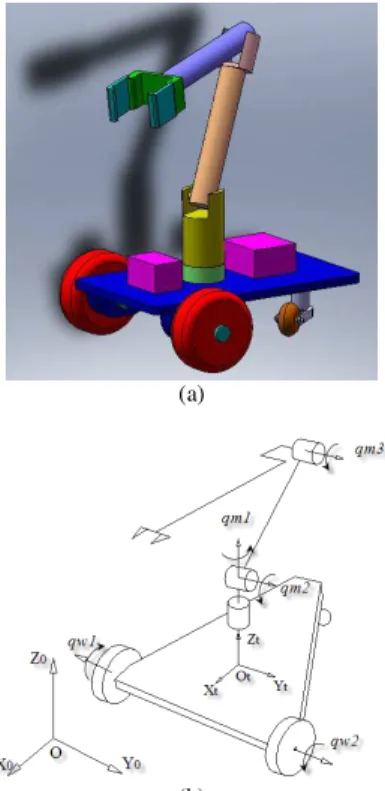
In this paper, we use a prototype of mobile manipulator with three degrees of freedom manipulator mounted on a nonholonomic mobile robot, shown in Fig. 1(a). The two independent driven wheels are cylindrical and equipped parallel to each other. Additionally, one caster wheel is fixed. The labels in Fig. 1(b) show the prototype of the revolute joints of robot in this work and the coordinate frames configuration of the mobile manipulator is shown in it. We denote the wheel, the trunk and the manipulator with subscripts w, t, m, respectively.
Under pure rolling condition, the constraint equation to the nonholonomic mobile manipulator subjected is given by
( )
qq=0A (1)
( )
∈ 1×6 R q(
)
T m m m t tt y q q q q x
q= , , , 1, 2, 3 (2)
From Eqs. (1) and (2), the dynamic equation can be given by the following equation:
( )
qqv Kq= (3)
( )
q M( )
qq H(
q,q)
G( )
q J( )
q FB τ = + + + T (4)
where
(
)
Tm m m w w
v q ,q ,q ,q ,q q = 1 2 1 2 3 ,
the matrix K
( )
q ∈R6×5 satisfies A( ) ( )
qKq =0 , B( )
q ∈R6×5 is input transformation matrix, τ∈R5×1 is the torque vector,( )
q ∈R6×6M denotes a inertia matrix, H
(
q,q)
∈R6×1 is centripetal and Coriolis vector, G( )
q ∈R6×1 denotes the gravitational vector,( )
∈ 6×6 R qJ T is a Jacobian matrix,F∈R6×1denotes the external force acted on the end-effector of manipulator.
(a)
(b)
Figure 1. (a) The nonholonomic mobile manipulator prototype. (b) Coordinate frames for the robot.
Stability Performance
The universe coordinate frame (O−XoYoZo) will be located according to the initial body-fixed coordinate frame (Ot−XtYtZt), shown in Fig. 1(b). For the planar stable supporting situation, we can fix a coordinate frame Z whose origin is ZMP located on the support plane, and its z-axis parallels with the normal vector of the support plane as shown in Fig. 2. The actual support polygon (ASP) represents a convex stable support polygon consisting of lines
connecting the support points. pi,ei denote the support point and the line vector.
Figure 2. The relation of ZMP location and the actual support polygon (ASP).
At any instantaneous time, there exists force equilibrium equation in the arbitrarily chosen body-fixed frame for the inertial force and the external force acting on the mobile manipulator system. The external force includes the gravity forces and the contact forces acted on the mobile robot system by environment. The equilibrium equation has the form
S M G I
F F F
F − − = (5)
where FI∈R6 , FG∈R6 , FM∈R6 and FS∈R6 are the resultant inertial force, the resultant gravity force, the resultant reaction manipulation force and the resultant supporting force for the robot system respectively.
The twist along the margin of ASP is the real cause of tip-over
for robot. FShas the vector form as
[
]
6R fT τT T∈ ,
[
]
3R f f f
fT = x y z T∈ ,
[
]
3R T z y x
T =τ τ τ ∈
τ .
The twist along ei induced by FScan be denoted as ui=
ξ
iTFS,(
)
[
T]
Ti T i i T i T
i e p ,e
e
× − ⋅ = 1
ξ .
Assuming the criterion LZMP∈ASP is satisfied, it means that FS will generate negative power along ei. Therefore, we can construct STC as
0 ≤
S T i F
ξ
(6)According to the above equations, the norm of uiimply the
least value of the twist which can tip over the robot along ei. We construct the optimization criterion to improve stability as follows.
( )
(
ui)
Minmax (7)
where uisatisfyui=Aiq+Bi,Ai∈R1×5andBi∈R1. A minimum performance function was constructed considering the property of the arithmetic and geometric mean inequality (Qiu et al., 2009). In this paper, we consider the property of the variance to formulate the performance function, as follows:
Subject to ui≤0 (9)
where i
u
u=
∑
i i , the minimum of Eq. (8) requires ui = uj . Therefore, the optimized solution of the system will make sure that the ZMP is located in the center of ASP in theory.Optimized Planning
The limits of the joints’ range, velocity and acceleration should
be considered in trajectory planning. Let ql∈R3×1 and qu∈R3×1 denote the lower and upper limits of the joints’ range (only the
joints of manipulator are considered), ql∈R5×1 and qu∈R5×1 represent the lower and upper limits of the joints’ velocity and
1 5×
∈R
ql and qu∈R5×1 denote the lower and upper joints’ acceleration limits. In order to use QP algorithm, the limits of the joints’ range, velocity and acceleration should be combined to a matrix form; then AJ and BJ for joint velocity constraints have the form 5 26 3 3 5 5 5 5 0 0 × − − − = I I I I I I
AJ (10)
(
)
(
)
( )
( )
1 26× − − − ⋅ − − − ⋅ + − − = t t q q t t q q q t t t q q t t t q q q B l u l u l u J ∆ ∆ α ∆ ∆ α ∆ ∆ (11) where[
]
m m m diag , , RI = 1 1∈ × and
[
α1 α5]
α =diag , , ,
(
0<α≤1)
.The joint torque limits can be indirectly realized by adjusting
α
and replacing ql and quwith the on-line minimum and maximum acceleration output under the joint torque limits. Eq. (8) can be transformed to a quadratic formulation.
Minimize uTΛu (12)
− − − − − − − − − = 1 1 1 1 1 1 1 1 1 i i i Λ (13)
where u=
[
u1, ,ui]
T∈Rn×1, u=ATq+BT.Combing Eq. (8)-Eq. (13), the optimized solution with tip-over prevention consideration for mobile manipulator can be constructed:
Minimize
⋅ = u q M u q H T Λ λ 0 0 (14)
Subject to
=
− n T
T B x u q I A J 0 (15) ≤ 0 0 0 J n J B u q I A (16)
where M is the inertia matrix and
λ
≥0 is a scalar weight which is used to adjust the tradeoff impact to the kinetic energy of the robot system for tip-over prevention. If the robot is static,λ
will be zero. When one component of u approaches zero, the high-level mission re-planning algorithm must be activated to avoid the danger mission.Simulation
Numerical simulations for the nonholonomic mobile manipulator presented above were performed. We present two simulation results for demonstrating the feasibility of improving the stability of nonholonomic mobile manipulator with STC consideration. The simulation results are depicted in Fig. 3 and Fig. 4 respectively. The nonholonomic mobile manipulator parameters are given in Table 1.
The two simulation examples adopt the same desired trajectory of the end-effector of manipulator. The initial world coordinates frame is chosen with the origin located on the support plane and the orientation parallels the body-fixed coordinate frame. The desired path of the end-effectors is designed as moving along a curve in T =10 s from the initial position to the termination. The curve is designed as x
( )
t x cos(
t /T)
3T25 1 0 ⋅ ⋅ − + = π π
, y
( )
t =y0 ,( )
t z cos(
t /T)
Tz = + − ⋅ ⋅
π π 40
2 1
0 in world coordinates frame. In the
first simulation the initial parameters are
(
)
T, , , , ,
q= 00180 −120 −30 −100 , while
(
)
T, , , , ,
q= 000 60 −30 −100 in the second simulation,
α
i =1. The sample time is 0.02 s. The ASP is constructed with three points in the body-fixed frame; the coordinates of the points are[
]
T. , . , .
p1= 007−012−01 , p2 =
[
−0.14,0,−0.1]
T ,[
]
T. , . , .
p3= 007012−01 .
The performance function is defined as the sum of the kinetic energy and the weighted vector norm of u . λ is defined asλ=λ0⋅
(
sin(
t⋅π/T)
)
, where λ0=0.005 and is chosen mainly considering the tradeoff with the kinetic energy by a trial-and-error process.initial state in two simulations, the constraint of mobility will induce the axis of driven wheel perpendicular to the desired velocity which will change the orientation of mobile base, shown in Fig. 3(e) and Fig. 4(e). It can be implicated by the noholonomic mobile constraint Eqs. (1) and (3). This characteristic is useful for us to fix equipments such as different sensors on a proper position of the nonholonomic mobile base. Moreover, it can be used to plan the trajectory of end-effector for obtaining more stable movements of nonholonomic mobile manipulator.
Conclusion
In this article, we investigate the dynamic stability of a nonholonomic mobile manipulator with STC consideration. The
dynamics of the nonholonomic mobile manipulator is derived. The performance function considering the property of the variance is formulated. The stability of nonholonomic mobile manipulators is improved with STC consideration. Comparing to the holonomic mobile base, the constraint of movement of nonholonomic mobile base will affect the orientation of mobile base. This characteristic should be considered in fixing the equipments on a proper position of the mobile base and re-planning a desired trajectory of end effector in order to improve stability of robot. Future work will focus on improving the stability by considering the forces from the load that is carried by the end-effector and the obstacle avoidance. The work of producing a real robot is progressing, and the experiments can be carried out using a real robot in the future.
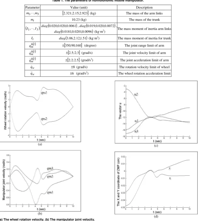
Table 1. The parameters of nonholonomic mobile manipulator.
Parameter Value (unit) Description
3
1, ,m
m ⋅⋅⋅
[
2.321;2.15;2.923]
(kg) The mass of the arm linkst
m 10.23(kg) The mass of the trunk
(
I1,⋅⋅⋅,I3)
(
0.020,0.020,0.0061)
diag ,diag
(
0.019,0.020,0.0072)
,(
0.0181,0.0201,0.0096)
diag (kg·m2) The mass moment of inertia arm links
t
I diag
(
3.06,2.12,1.51)
(kg·m2) The mass moment of inertia for trunk( )l h m
q ±
[
350;90;160]
(degree) The joint range limit of arm( )l h m
q ±
[
2.5;2;3]
(grad/s) The joint velocity limit of arm( )l h m
q ±
[
2;2;2.5]
(grad/s2) The joint acceleration limit of armw
q ±8 (grad/s) The rotation velocity limit of wheel
w
q ±6 (grad/s2) The wheel rotation acceleration limit
(a)
(b)
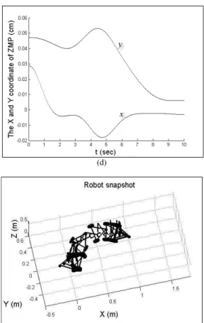
Figure 3. (a) The wheel rotation velocity. (b) The manipulator joint velocity. (c) The norm of vector u. (d) The X and Y coordinate of the ZMP in the body fixed frame. (e) The snapshot of the robot movement process.
(c)
(d)
(e)
Figure 3. (Continued).
(a)
(b)
(c)
Figure 4. (a) The wheel rotation velocity. (b) The manipulator joint velocity. (c) The norm of vector u. (d) The X and Y coordinate of the ZMP in the body fixed frame. (e) The snapshot of the robot movement process.
(d)
(e)
Figure 4. (Continued).
Acknowledgements
The work presented in this paper is supported by the 863 National High-Tech Program of China (Grant No. 2006AA04Z261).
References
Brock, O. and Khatib, O., 2000, “Real-time replanning in high-dimensional configuration spaces using sets of homotopic paths”. Proc. of the ICRA IEEE Intl. Conf. on Robotics and Automation, San Francisco, CA, Vol. 1, pp. 550-555.
Brock, O., Khatib, O. and Viji, S., 2002, “Task-consistent obstacle avoidance and motion behavior for mobile manipulation”. Proc. of the ICRA IEEE Intl. Conf. on Robotics and Automation, Washington, DC, Vol. 1, pp. 388-393.
Cheng, F.-T., Chen, T.-H., and Sun, Y.-Y., 1992, “Efficient algorithm for resolving manipulator redundancy-the compact QP method”. Proc. of the ICRA IEEE Intl. Conf. on Robotics and Automation, Vol. 1, pp. 508-513.
Cheng, F.-T., Chen, T.-H., Wang, Y.-S., and Sun, Y.-Y., 1993, “Obstacle avoidance for redundant manipulators using the compact QP method”. Proc. of the ICRA IEEE Intl. Conf. on Robotics and Automation, Vol. 3, pp. 262-269.
Cheng, F.-T., Sheu, R.-J., Chen, R.-H., and Kung, F.-C., 1994, “The improved compact QP method for resolving manipulator redundancy”, Proc. of the IROS IEEE/RSJ/GI Intl. Conf. on Intelligent Robots and Systems, Vol. 2, pp. 1368-1375.
Furuno, S., Yamamoto, M. and Mohri, A., 2003, “Trajectory planning of mobile manipulator with stability considerations”. In: Proc. of the ICRA IEEE Intl. Conf. on Robotics and Automation, Taipei, Taiwan, Vol.3, pp. 3403–3408.
Huang, Q., Tanie, K. and Sugano, S., 1999, “Stability compensation of a mobile manipulator by manipulator motion: feasibility and planning”,
Advanced Robotics, Vol. 13, No. 6-8, pp. 25-40.
Khatib, O., 1987, “A unified approach for motion and force control of robot manipulators: the operational space formulation”, IEEE Journal of Robotics and Automation, Vol. 3, No. 1, pp. 43-53.
Kim, J., Chung, W.K., Youm, Y. and Lee, B.H., 2002, “Real-time ZMP compensation method using null motion for mobile manipulators”. In: Proc.
of the ICRA IEEE Intl. Conf. on Robotics and Automation,Washington, DC, Vol. 2, pp. 1667-1972.
Qiu, C., Cao, Q., Yu, L., and Miao, S-H., 2009, “Improving the stability level for on-line planning of mobile manipulators”, Robotica, Vol. 27, No. 3, pp. 389-402.