Doutor Pedro Alexandre da Costa Sousa

Low Cost Inertial-based Localization System for a Service

Robot

Rúben José Simões Lino

Dissertação apresentada na Faculdade de Ciências e Tecnologia da Universidade Nova de Lisboa para a obtenção do grau de

Mestre em Engenharia Electrotécnica e de Computadores

Orientador

:

Doutor Pedro Alexandre da Costa Sousa

Júri

Presidente:

Doutor José António Barata de Oliveira

Vogais:

Doutor João Paulo Branquinho Pimentão

Doutor Pedro Alexandre da Costa Sousa

iii

UNIVERSIDADE NOVA DE LISBOA

Faculdade de Ciências e Tecnologia

Departamento de Engenharia Electrotécnica e de Computadores

Sistema de Localização Inercial de Baixo Custo para um

Robô de Serviço

Por:

Rúben José Simões Lino

Dissertação apresentada na Faculdade de Ciências e Tecnologia da Universidade Nova de Lisboa para a obtenção do grau de

Mestre em Engenharia Electrotécnica e de Computadores

Orientador:

Prof.

Pedro Alexandre da Costa Sousa

v

NEW UNIVERSITY OF LISBON

Faculty of Sciences and Technology

Electrical Engineering Department

Low Cost Inertial-based Localization System for a Service

Robot

Rúben José Simões Lino

Dissertation presented at Faculty of Sciences and Technology of the New University of Lisbon to attain the Master degree in Electrical and Computer Science Engineering

Supervisor:

Prof. Pedro Alexandre da Costa Sousa

vii

Low Cost Inertial-based Localization System for a Service Robot

Copyright © Rúben Lino, FCT/UNL e UNL

ix

Acknowledgements

For all persons that, in some way, had contributed to this dissertation I want to express my deepest acknowledgments.

First of all I want to manifest a sincerely gratitude to Prof. Pedro Sousa, my dissertation supervisor, for providing the conditions to do this work, giving me this opportunity and for all advices and guidance along the way.

I can not forget my colleagues Pedro Gomes and Tiago Ferreira for all the interesting discussions, critics, comments and casual talking. To João Lisboa I have to thank all the wise observations and special critics and also his availability. Non forgetting also all my university friends and coworkers of Holos, SA.

I would like to thank Neuza from all of comprehension, support and encouragement that she always transmitted me, even along the toughest times.

xi

Abstract

The knowledge of a robot’s location it’s fundamental for most part of service robots. The success of tasks such as mapping and planning depend on a good robot’s position knowledge.

The main goal of this dissertation is to present a solution that provides a estimation of the robot’s location. This is, a tracking system that can run either inside buildings or outside them, not taking into account just structured environments. Therefore, the localization system takes into account only measurements relative.

In the presented solution is used an AHRS device and digital encoders placed on wheels to make a estimation of robot’s position. It also relies on the use of Kalman Filter to integrate sensorial information and deal with estimate errors.

The developed system was testes in real environments through its integration on real robot. The results revealed that is not possible to attain a good position estimation using only low-cost inertial sensors. Thus, is required the integration of more sensorial information, through absolute or relative measurements technologies, to provide a more accurate position estimation.

xiii

Resumo

O conhecimento da sua localização é fundamental para a maior parte dos robôs de serviço. O sucesso de funções como construção de mapas e planeamento dependem de um bom conhecimento sobre a posição do robô.

O principal objectivo desta dissertação é apresentar uma solução que realize uma estimativa sobre a localização do robô. Um sistema de localização capaz de funcionar quer dentro de edifícios quer no seu exterior não tendo em conta ambientes estruturados. Deste modo, o sistema de localização tem em conta, somente, medições relativas.

Na solução apresentada é utilizado um dispositivo AHRS e encoders digitais nas rodas para realizar uma estimativa da posição do robô. Recorre-se ainda à utilização de Filtro de Kalman para integrar informação sensorial e lidar com erros provenientes da estimativa.

O sistema desenvolvido foi testado em ambientes reais através da sua integração num robô físico. Os resultados indicam que não é possível obter uma boa estimativa de localização utilizando apenas sensores inerciais de baixo-custo. Sendo necessária a integração de informação sensorial, através de medidas absolutas ou relativas, de modo a fornecer uma estimativa com menos erro.

xv

Contents

1. Introduction ... 1

1.1 Problem Statement ... 2

1.2 Solution Prospect ... 3

1.3 Dissertation Outline ... 3

2. State of the Art ... 5

2.1 Absolute Position Measurements ... 5

2.1.1 Wireless ... 5

2.1.2 Landmarks ... 9

2.2 Relative Position Measurements ... 10

2.2.1 Inertial measurement unit ... 11

2.2.2 Odometry ... 11

2.3 Robot Localization ... 12

3. Supporting Concepts ... 19

3.1 Coordinate Systems used in Inertial Navigation ... 19

3.2 Coordinate Systems Transforms ... 22

3.2.1 Direction Cosine Matrix – Rotation Matrix (RPY to NED) ... 22

3.2.2 NED/ECEF and ENU/ECEF Transformations ... 25

3.2.3 Transformation between ECEF and ECI ... 26

3.3 Navigation Equations ... 27

3.3.1 Earth frame mechanization ... 29

3.3.2 Local frame mechanization ... 30

3.4 Strapdown Inertial Navigation Systems ... 31

3.5 Kalman Filter... 33

3.5.1 Computational Consideration ... 34

3.5.2 Kalman Filter Algorithm ... 35

3.6 Player ... 38

4. Localization Solutions ... 41

xvi

4.1.1 Acceleration Corrections ... 43

4.2 Kalman filter ... 45

4.3 Player Integration ... 49

5. Experimental Results ... 51

5.1 Equipment ... 51

5.2 Tests ... 55

5.2.1 Indoor - straight line ... 56

5.2.2 Circular Trajectories ... 61

5.2.3 Closed Circuit ... 64

6. Conclusions and Future Work ... 69

6.1 Conclusions ... 69

xvii

List of Figures

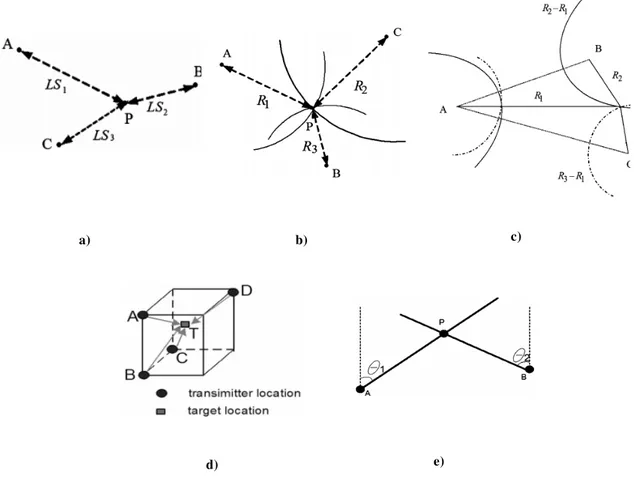
Figure 2.1 – a) positioning based on RSS, where LS1, LS2 and LS3 denote measured path loss; b) positioning based on TOA/RTOF measurements; c) positioning based on TDOA measurements; d) positioning based on signal phase; e) positioning based on AOA; adapted from Liu et al. [Liu et

al., 2007]... 6

Figure 2.2 - Overview of principal positioning wireless techniques [Liu et al., 2007] ... 7

Figure 2.3 - Two possible methods to detect artificial landmarks: (a) laser beam is sent towards the landmark and received; (b) the landmark is detected by the omnidirectional camera image. ... 10

Figure 2.4 - Single axis odometry ... 11

Figure 2.5 - UWB and GPS errors [González et al., 2009] ... 13

Figure 2.6 - Structure of Panzieri et al. localization system. ... 14

Figure 2.7 - Multi-aided inertial navigation system developed by Liu et al. [Liu et al., 2005] ... 15

Figure 2.8 - a) testing environment; b) the general paths from three methods [Liu et al., 2005] ... 16

Figure 3.1- Representation of latitude and longitude. ... 20

Figure 3.2 - ECI and ECEF coordinate systems ... 20

Figure 3.3 - ENU coordinate system [Grewal, 2001] ... 21

Figure 3.4 - RPY coordinate system [Grewal, 2001]... 21

Figure 3.5 - Example of coordinate system transform ... 22

Figure 3.6 - Rotation over Z axis ... 24

Figure 3.7 - Rotation over Y axis ... 24

Figure 3.8 - Rotation over X axis ... 24

Figure 3.9 - Representation of NED coordinate system on ECEF ... 25

Figure 3.10 - Diagram showing the components of the gravitational field [Titterton, 2004] ... 29

Figure 3.11 - Orthogonal instrument cluster arrangement, adapted from Titterton [Titterton, 2004] ... 32

Figure 3.12 - Inertial Navigation System representation, adapted from Titterton [Titterton, 2004] ... 32

Figure 3.13 - The cycle of discrete Kalman filter algorithm [Welch, 2006]. Time update predicts the current state estimate while measurement update corrects the projected estimate using the measured data. ... 36

Figure 3.14 - A complete picture of the Kalman filter algorithm [Welch, 2006] ... 37

Figure 3.15 – General structure of Player. ... 38

Figure 3.16 - The Run-Time Layout of a Player Driver [PsuRobotics, 2010] ... 40

xviii

Figure 4.2 - Specific structure of Player for position estimation ... 49

Figure 4.3 - Run-time process of CalcPosDriver, adapted from Gomes [Gomes, 2010] ... 50

Figure 5.1 - Platform in which localization system is implemented ... 51

Figure 5.2 - XSens MTi inertial sensor ... 52

Figure 5.3 - the motor controller - Roboteq AX3500 ... 54

Figure 5.4 - The optical digital encoders used in the robot ... 54

Figure 5.5 - Tests' circuit ... 56

Figure 5.6 - 20 meters indoor with double integration algorithm: (a) the xy trajectory (b) the yaw variance over time... 57

Figure 5.7- double integration algorithm behavior in 20 meters indoor test: (a) acceleration; (b) speed; (c) position ... 58

Figure 5.8 - Velocity read by encoders ... 58

Figure 5.9 - 20 meters indoor with Kalman filter: (a) the xy trajectory; (b) the yaw variance over the distance (c) the roll variance over the distance; (d) the pitch variance over the distance ... 59

Figure 5.10 – One dimension’s test – real distance versus estimated distance ... 60

Figure 5.11 - Error amount over the distance ... 60

Figure 5.12 - anti-horary circular trajectory with Kalman filter: (a) the xy trajectory; (b) the yaw variance over the distance (c) the roll variance over the distance; (d) the pitch variance over the distance ... 62

Figure 5.13 - X position versus the velocity received from motor controller driver ... 63

Figure 5.14 - Horary circular trajectory with Kalman filter: (a) the xy trajectory; (b) the yaw variance over the distance (c) the roll variance over the distance; (d) the pitch variance over the distance ... 64

Figure 5.15 - closed circuit trajectory with Kalman filter: (a) the xy trajectory; (b) the yaw variance over the distance (c) the roll variance over the distance; (d) the pitch variance over the distance ... 65

xix

List of Tables

Table 1 - Some WLAN-based indoor positioning systems and solutions, adapted from Liu et al

[Liu et al., 2007] ... 7

Table 2 – Some UWB indoor positioning systems and solutions, adapted from Liu et al [Liu et al., 2007]... 8

Table 3 – Some RFID-based indoor positioning systems and solutions... 8

Table 4 - Agrawal et al. results: loop closure error in percentage ... 14

Table 5 - Liu et al. errors from IMU and aided IMU methods. ... 16

Table 6 - Estimation errors (in meters) in correspondence of the marker configurations (distance between the marker and estimated position) [Ippoliti et al., 2005] ... 16

Table 7 – Santana’s results for the three different Kalman filter configuration. ... 17

Table 8 - Attitude and heading accuracies ... 52

Table 9 - Individual sensor specifications ... 53

Table 10 – Sensor’s type used in MTi ... 53

xxi

Symbols and Notations

Symbols Description

AHRS Attitude and Heading Reference System AOA Angle Of Arrival

DGPS Differential Global Positioning System DTG Dynamically Tuned Gyroscope

ECEF Earth Centered Earth Fixed ECI Earth Centered Inertial ENU East-North-Up

FOG Fiber Optic Gyroscope GPS Global Positioning System

IFR International Federation of Robotics IMU Instrument Measurement Unit

INS Inertial Navigation System kNN k-Nearest Neighbor LPT Local Tangent Plane

MEMS Microelectromechanical Systems NED North-East-Down

RFID Radio Frequency Identification RPY Roll-Pitch-Yaw

RSS Radio Signal Strengths RTOF Roundtrip Time Of Flight

SLAM Simultaneous Localization and Mapping SMP Smallest M-vertex Polygon

SVM Support Vector Machine TDOA Time-Difference Of Arrival

TOA Time of Arrival UWB Ultra-Wide Band

F Specific force vector A Acceleration vector

G Gravitational acceleration vector Roll Angle

xxii Angular speed

Angular speed of the Earth L Latitude

Longitude H Altitude

Transformation matrix from ECEF to NED Transformation matrix from NED to ECEF Transformation matrix from ECI to ECEF Estimate error covariance matrix

Process noise covariance matrix Measurement noise covariance matrix State transition matrix

1

1.

Introduction

In earlier 20th century, more precisely in 1920, the word robot was introduced by Karel Capek in his play RUR, Rossum’s Universal Robot. Capek’s idea of these beings was that robots were artificial automated workers with their own soul, but they were meant to serve. Since then, the development in robotic area allowed the use of robots in diverse areas making them an integrating part of our society.

In these days, robots are helping humans in monotonous, dangerous and difficult to achieve (like accurate or heavy weight related) tasks. Cleaning and housekeeping, elderly care, interplanetary exploration, humanitarian demining, tour-guide, underwater exploration and surveillance are some possible applications of a robot.

“From static, non-autonomous robots in the beginning, robots now become more and more mobile and autonomous” [Negenborn, 2003]. Autonomy and mobility are such important characteristics for robots that need to move freely to do their tasks, like service robots. The International Federation of Robotics (IFR) defines a service robot as “(…) a robot which operates semi- or fully autonomously to perform services useful to the well-being of humans and equipment, excluding manufacturing operations” [IFR, 2009].

Navigation is a task that service robots must be able to do. Navigation can be divided in localization, obstacle detection and avoidance and planning . Therefore, they can move safely from its location to another one. According to Leonard and Whyte [Leonard and Durrant-Whyte, 1991], the general proposition of navigation can be resumed in three questions: “where am I?”, “where am I going?” and “how should I get there?”.

The question “where am I?” is the focus of this thesis and relies with robot localization, which is one of the problems of service robots. Once autonomy and mobile are principal features of these robots, the knowledge about robot’s position and orientation is absolutely needed. Thus, it is possible to solve other problems such as mapping, obstacle avoidance and planning and, thereby, have an approach to answer the problem of navigation.

It’s common to see localization issues being solved by technologies like GPS, inertial systems or vehicle’s odometry,

2

Its major disadvantage is that the environment has to be structured because this kinds of technologies need to be placed in vehicle and outside it. This means that references have to be placed strategically (in the environment where the robot will operate) in order to have a better error/cost relation. With low price and accuracy of these days’ GPS technology these measurements are, essentially, applied in indoor environments where GPS is unsuitable.

Nowadays, location is usually obtained from combining the short-term accuracy of relative measurements methods with the time-independent bounded error of the absolute measurements methods. ”The actual trend is to exploit the complementary nature of these two kinds of sensorial information to improve the precision of the localization procedure” [Ippoliti et al., 2005].

Simultaneous localization and Mapping is being, in these days, a subject of research in mobile robots area. The basic idea of SLAM is to place an autonomous vehicle at an unknown location in an unknown environment and have it build a map, using only relative observations, and then using this map to navigate [Dissanayake et al., 2001]. However, this thesis doesn’t try to contribute to this field of research.

In this work, the goal is to answer the question “where am I?” using only dead-reckoning systems1. A reliable estimate of a robot’s will be attempted with a low-cost inertial measurement unit as main sensor. Furthermore, sensorial odometric information will be added to improve the estimate’s precision.

A priori, it is possible to say that this error will be unbounded along the time since won’t be used absolute position measurements.

1.1

Problem Statement

The main goal of this dissertation is to present a localization solution including only relative measurements of an attitude and heading reference system and digital encoders placed in wheels. Indoor and outdoor environments are included once the system only relies in relative measurements. Therefore, systems such as GPS, which is widely used to do localization, is discarded and a low cost inertial measurement unit and digital encoder information will be used.

The rotational speed of the Earth is one problem of localization through a strapdown inertial system once that it inflicts particular forces that cause noise on acceleration and gyroscopes (gyroscope drift). These particular forces are known as local gravitational force and Coriolis acceleration.

1

3

Dead-reckoning systems have as main disadvantage the cumulative error of position. So it is needed a method that deals with errors and could combine the data from various sources.

Another problem is information integration of various sources. It is needed to acquire data from sensors in real-time in order to do a better estimation of position.

1.2

Solution Prospect

In this thesis will be presented different solutions that will use a inertial measurement unit and digital encoders placed on wheels. This combined with navigation equations and Kalman filters will provide some position estimations.

To correct acceleration by the influences of the Earth’s movement it will be implemented the navigation equations. It takes in account the rotational speed of the earth to translate the platform’s acceleration to an Earth fixed frame. With navigation equations it is possible to know the exact value of Coriolis acceleration and local gravitational force and, thus, deduct it to the acceleration vector.

Kalman filter is a tool widely use in control and prediction areas and also in autonomous or assisted navigation. It uses the all available information to predict the state of system and to project the error ahead. After that, with complemental measurements it corrects the estimate. In this way, it will be used a Kalman filter to estimate the robot’s position and dealing with cumulative dead-reckoning errors.

To attempt to solve the localization of a mobile robot, with an inertial sensor as the main reference, will be implemented and tested two methods: an algorithm referred as double integration algorithm, which only uses the data provided by inertial sensor combined with navigation equations to obtain a estimate of robot’s velocity and position; Kalman filter appears as another solution, implementing it with data received from inertial sensor and aided by velocity obtained by digital encoder. All of this, integrated in a Player module.

The Player is a software tool capable of communicate with hardware normally used in robot’s projects. It is modular, this means that it’s separated in different logical modules which helps the integration of new modules (such as drivers or algorithms). It has itself a messaging system to communicate between modules.

1.3

Dissertation Outline

4

Chapter 1: introduces the reader to the problem of robot localization;

Chapter 2: exposes a brief overview of the state of the art about localization in general and then giving the focus to robot localization;

Chapter 3: provides an overview of supporting mechanisms used in robot localization;

Chapter 4: description of algorithms implemented;

Chapter 5: presents the experimental results;

5

2.

State of the Art

In this Chapter will be presented and discussed the main techniques to do mobile robot localization. In section 2.1 there are the most common techniques to do localization using absolute position measurements, in section 2.2 will be described localization techniques using relative position measurements. In section 2.3 are presented localization methods that combine relative position measurements with absolute position measurements to achieve a more accurate estimate of position.

Over the years, with the development of robotic industry and appearance of mobile robots the robot localization became an emergent problem to solve. Since then, a variety of systems, sensors and techniques for mobile robot positioning are being subject of interest for researchers and engineers. According to Borenstein et al. [Borenstein et al., 1997], an accurate knowledge of a vehicle’s position is fundamental in mobile robot application.

Borenstein et al. divides the localization techniques into Relative Position Measurements and Absolute Position Measurements [Borenstein et al., 1997]. He also refers to Relative Position Measurements as dead-reckoning and to Absolute Position Measurements as reference-based systems.

2.1

Absolute Position Measurements

Absolute localization requires a structured environment where the robot is operating. Having sensors in the robot (under a structured environment) providing data to it or have some outside references that help localizing robot is considered as absolute measurements. Among the most known and used are the GPS and other wireless systems (such as WLAN, cellular based and UWB). Another system widely use in robot localization is the usage of landmarks which could be natural (such as trees and room corners) or artificial (barcodes, pattern images, etc…).

2.1.1

Wireless

6

common to use triangulation, positioning algorithms using scene analysis or proximity methods in order to have an estimate for location discarding the measurement errors.

a) b) c)

d) e)

Figure 2.1 – a) positioning based on RSS, where LS1, LS2 and LS3 denote measured path loss; b) positioning

based on TOA/RTOF measurements; c) positioning based on TDOA measurements; d) positioning based on signal phase; e) positioning based on AOA; adapted from Liu et al. [Liu et al., 2007]

Shortly, triangulation is based on geometric properties of triangles to estimate the target location. It could be divided in lateration and angulation. Lateration estimates the position of an object by measuring its distance from multiple reference points (it includes RSS-based, TOA – Time of Arrival, TDOA – Time difference of Arrival, RTOF – Roundtrip Time of Flight and received signal phase method). In angulation techniques (AOA) the location of the target is estimated by the intersection of several pairs of angle direction lines. Liu et al. gives an more precise explanation of these techniques [Liu et al., 2007].

7

probabilistic methods, k-nearest neighbor (kNN), neural networks, support vector machine (SVM) and smallest M-vertex polygon (SMP).

Proximity algorithms are very simple to implement and provide symbolic relative location information [Liu et al., 2007]. The simplest application of proximity is when a mobile target is detected by a single antenna and, knowing the location of antenna, it’s possible to have an approximate location of mobile target. Infrared radiation (IR), radio frequency identification (RFID) and cell identification (Cell-ID) are some proximity localization methods.

Wireless systems are common used in indoor localization. Liu et al., provides an overview of the existing wireless indoor positioning solutions, explaining the different techniques and systems such as WLAN, RFID, UWB, GPS, Bluetooth, Ultrasounds, ZIGBEE and GSM. In Figure 2.2 it’s presented the principal wireless location systems and its accuracy. Some of these will be approached ahead.

Figure 2.2 - Overview of principal positioning wireless techniques [Liu et al., 2007]

WLAN

As referred before, scene analysis’ methods are widely used in wireless systems. In WLAN localization the most common technique is fingerprinting location with radio signal strengths.

System/solution Wireless technology Positioning algorithm accuracy Precision

Microsoft Radar RSS kNN 3-5m 50% within around 2.5m and

90% within around 5.9m

DIT RSS MLP, SVM 3m 90% within 5.12m for SVM

and 90% within 5.4m for MLP

Ekahau RSS Probabilistic method 1m 50% within 2m

MultiLoc RSS SMP 2.7m 50% within 2.7m

8

The system developed by Caceres et al. is one example of scene analysis method. They’ve developed a WLAN-based real time vehicle location system [Caceres et al., 2009]. Using as positioning algorithm a trained neural network with a map of received power fingerprints from WLAN Access Points, they have an approximate error of 7 meters.

UWB

As indicated in Figure 2.2 Ultra-Wide Band is one of the best resolution wireless localization system. UWB is based on sending ultrashort pulses [Liu et al., 2007]. It uses frequencies from 3.1 to 10.6 GHz and transmits simultaneously a signal over the multiple bands. As well as the others wireless systems used in location, UWB sensors must be placed at known places and techniques as TDOA and AOA (or both together) are used to obtain a real-time 2D or 3D position. UWB location exploits the characteristics of time synchronoization of UWB communication to achieve a very high indoor localization (20 cm).

It short duration pulses are easily filtered and determined which signals are correct and which derive from multipath. The signal of UWB passes easily through walls, equipment and clothing, but has metallic elements or liquid materials will cause interferences on signal.

A well known system is the one developed by Ubisense. Using a combination of TDOA and AOA it provides and 2D/3D position with an accuracy of 15 cm where 99% of time with an error below of 0.3 m [Liu et al., 2007]. González et al. developed a combination of UWB and GPS for indoor-outdoor vehicle localization [González et al., 2009] that will be focused in section 2.3.

System/solution Wireless technology Positioning algorithm accuracy Precision

Ubisense UWB (TDOA+AOA) Least Square 15 cm 99% within 0.3m

Sappire Dart UWB (TDOA) Least Square <0.3m 50% within 0.3m

Table 2 – Some UWB indoor positioning systems and solutions, adapted from Liu et al [Liu et al., 2007]

RFID

Using RFID it’s possible to determine the location of an object through proximity or scene analysis methods. Using passive tags placed at known locations and a reader placed in the object it’s possible to know approximate position of the object. LANDMARC [Ni et al., 2004] and SpotON [Hightower et al., 2000] methods use active tags and fingerprinting locating through RSS.

System/solution Wireless technology Positioning algorithm accuracy Precision

SpotON Active RFID RSS Ad-Hoc Lateration Depends on the

size of cluster N/A

LANDMARC Active RFID RSS kNN 3m 50% within 1m

9 GPS

Global Positioning Systems (GPS) are, probably, the most used approach to do navigation. It was developed by the US Department of Defense. The system is composed by 24 satellites in the Earth’s orbit and ground stations. The position of the GPS receiver is computed based on the principle of trilateration after receiving information about satellites’ localization combined with the time of flight of radio frequency signal [Ashkenazi et al., 2000].

In mobile robot localization is not very common it appears a stand-alone method to do localization or navigation once that it could only be used outdoors in areas covered by technology’s satellites. In urban of dense forest environments the GPS suffers from signal blockage and multipath interference. Besides, a regular GPS provides an accuracy of <10m [Ashkenazi et al., 2000] which, could not match the requirements of application.

There is an augmentation of this technology which is, commonly, used in mobile robot localization – DGPS. The Differential Global Positioning System has a pre-determined reference stations and can offer an accuracy of 1-2m [Ashkenazi et al., 2000]. Because of the poor coverage of signal for indoor environments its accuracy is low and it is unsuitable to be used to indoor position estimation. Another augmentation developed to overcome limitations of conventional GPS is the A-GPS (Assisted GPS). Using a location server with a reference GPS receiver, it combines the weak GPS signals with mobile station (or wireless handset) in order to produce a position estimate. It has 5-50 m accuracy in indoor environments [Liu et al., 2007].

Because it is widely used its price is decreasing over the time, which is, associated to characteristics, probably the main advantage. In other side, the incapacity of being used indoors is one of its problems.

2.1.2

Landmarks

In indoor or outdoor environments landmarks utilization is a very common method used in mobile robot localization since robots became mobile and autonomous. Basically, there are two kinds of landmarks: natural and artificial landmarks. Natural landmarks are those objects or features that are already in the environment and have a function other than robot navigation while artificial landmarks are specially designed to do navigation and placed in the specific locals with this unique propose [Borenstein et al.,1997].

10

In these methods the environment has to be structured. This is, the landmarks have to be placed at known locations in order to known the robot’s position when it sees the landmarks. These landmarks can be detected in various ways. The usage of an omindirectional camera (Figure 2.3 a)) or a rotating laser beam (Figure 2.3 b)) are two possible methods and they are illustrated on Figure 2.3

(a) (b)

Figure 2.3 - Two possible methods to detect artificial landmarks: (a) laser beam is sent towards the landmark and received; (b) the landmark is detected by the omnidirectional camera image.

In both cases the sensor used must be mounted on robot. The usage of laser beams or cameras makes allows to identify the landmarks and measure their bearings. Using a laser scanner and artificial landmarks made of retro-reflective material so they can be detected easily detected by photodetector. According to Loevsky and Shimshoni the landmarks can be single-stripped or in form of a barcode [Loevsky and Shimshoni, 2010]. In form of a barcode the returning beam is analyzed and landmarks can be identified. To identify landmarks using an omnidirectional camera (Figure 2.3 b)) the captured image has to be processed and landmarks must be distinguishable from other objects in the scene for an image processing algorithm can detect them.

The orientation of the robot can be obtained measuring the bearings of the landmarks and location is then obtained by triangulation.

2.2

Relative Position Measurements

11

2.2.1

Inertial measurement unit

Inertial measurement units consist in having a set of accelerometers and a set o gyroscopes. Both disposed orthogonally in order to obtain inertial accelerations and angular speeds in the three axes.

Through the acceleration and angular velocity obtained it’s possible to compute the variation of position and angle using the following equations:

=

=

Though, it is necessary the usage of methods to compensate the attitude of sensor and gravity. It is very common see inertial navigation system applications in ships, submarines, aircrafts, spacecrafts and guided missiles. They have the advantage of being self-contained and not jammable. However, inertial sensors are mostly unsuitable for accurate positioning over extended period of time [Borenstein et al., 1997]. Due to the price of high-quality INS it isn’t very common to use in robot applications. Thus, it is often used low-cost inertial sensors combined with other sensorial information as we will see in Section 2.3.

2.2.2

Odometry

Odometry is based on simple equations which hold true when wheel revelations can be translated accurately into linear displacement. Through wheel encoders’ information and using the vehicle’s correspondent kinematic model it is possible to know the velocity and position.

Figure 2.4 - Single axis odometry

12

digital encoder that counts the ticks, knowing the wheel’s radius ( ) and the ticks per revolution ( ) it’s possible to measure the number of ticks ( ) in a time interval ( ). So distance and speed are given, respectively, by:

!" = ∙ 2%

"" = !"

Nevertheless, in order to obtain 2D speed and distance information there is the need to implement the kinematic model of the robot which depends on its configuration.

Wheel slippage and cracks (systematic errors) or kinematic imperfections (non-systematic errors) are the main reason why this system is not so used alone [Borenstein et al., 1997]. Another type of odometry is using camera’s sequence image to compute de vehicle’s movement. This is a method which doesn’t suffer with wheel slippage. Normally, it is combined with other sensorial data. In Section 2.3 it is presented some methods that use odometry as complementary information.

2.3

Robot Localization

Once that in robot localization is wanted the most accurate knowledge of position appeared the need to combine different sensors and techniques resulting in, mostly, “hybrid” localization methods. This means that is, often, combined relative position measurements with absolute position measurements to achieve the robot’s position. This combination has the purpose of use the best of each group and hide its drawbacks: the difficulty of being always under structured environments and the error associated to the relative measurements position’s methods. Thus, it’s added the accuracy of absolute systems with the estimate (and independence of absolute measurements) of the relative methods.

Combination of Absolute Measurements Technologies

13

methods travelling in a indoor-outdoor circuit. The first one only relies on odometry, in the second the particle filter also has in consideration UWB and in the third GPS data is added to the particle filter. Figure 2.5 shows the errors of the three different methods over the time. The shadowed areas represent the part in navigation where GPS and UWB data were combined.

Figure 2.5 - UWB and GPS errors [González et al., 2009]

Combination of Absolute/Relative Measurements Technologies

Panzieri et al have presented an outdoor solution that fuses data from a GPS and from an inertial unit [Panzieri et al., 2002]. Their work presents a localization algorithm based on Kalman filtering that fuses information from an inertial platform and an inexpensive single GPS. It also uses map based data in their algorithm. In more details, their system have encoders measuring rotation of each motor, a inertial navigation system that provides measures of the robot linear accelerations and angular velocities, a laser scanner which measures the distances between a fixed point on the robot body and obstacle surfaces in the environment and a GPS measuring absolute position in the geodetic coordinates.

This work uses a very simple inertial model in the Kalman filter since inertial’ input is

14

Figure 2.6 - Structure of Panzieri et al. localization system.

Agrawal and Konolige refer that in outdoors an accurate position can be obtained using a differential GPS and/or a high-quality, expensive inertial navigation system [Agrawal and Konolige, 2006]. So they developed an inexpensive localization solution using stereovision and GPS complemented by IMU/vehicle odometry. They’ve tested three methods: a solution that combines IMU and vehicle odometry, visual odometry only by itself and visual odometry combined with GPS as referred before. In their tests the last method has showed the best performance followed by raw visual odometry. With the biggest percentage error appeared the position obtained by vehicle odometry combined with an inexpensive inertial navigation sensor.

Their system relies on stereo vision to estimate frame-to-frame motion in real-time. Aside, it uses a Kalman filter based on inertial measurements that fuses wheel encoders and GPS data to estimate the motion when visual odometry fails.

Table 4 shows the percentage of error for the three methods in the different closed-circuits. The principal characteristics of each one and conclusions of its results are discussed in their work.

Run number 1 2 3 4

Distance (meters) 82.4 141.6 55.3 51.0

Method Percentage Error

IMU-Vehicle Odometry 1.3 11.4 11.0 31.0 Raw Visual Odometry 2.2 4.8 5.0 3.9 Visual Odometry & GPS 2.0 0.3 1.7 0.9

15

Liu et al. say that mobile robot localization in the general outdoor conditions is much more difficult than fairly flat and structured indoor environments [Liu et al., 2005]. According with Liu et al. in the uneven surfaces wheels encoders suffers much larger systematic errors and the outdoor environments are often semi-structured or totally unstructured.

They developed a multi-aided inertial navigation system for outdoor ground vehicles which uses a Kalman filter to fuse data from an INS and two wheel encoders that provide data to a kinematic model in order to extract a velocity estimate to be used by the filter. Also has been used GPS data for INS/GPS method developed. The general idea of the filter for aided INS is presented in Figure 2.7.

Figure 2.7 - Multi-aided inertial navigation system developed by Liu et al. [Liu et al., 2005]

Although the system has been developed to outdoor environments and implemented on a pickup truck, the same idea (without GPS) could be applied to an indoor vehicle either once the system doesn’t use structured environments.

16

a) b)

Figure 2.8 - a) testing environment; b) the general paths from three methods [Liu et al., 2005]

North (m) East (m)

IMU 345 106

Aided IMU 3.7 7.5

Table 5 - Liu et al. errors from IMU and aided IMU methods.

Ippoliti’s et al. work is a low-cost localization system for a robot using only internal sensors, i.e., relative position measurements. Their system is composed by odometers and an optical fiber gyroscope.

They’ve presented 3 different algorithms. In the three methods is achieved x and y position’s estimate as well as robot’s orientation. In the first one the position’s estimate is only based on information received from wheels’ encoders and kinematic of vehicle.

In the algorithm 2 the orientation is calculated using angular measures of a fiber optic gyroscope. The x and y position’s estimate is computed applying this new orientation to the kinematic model used before. In

the third algorithm a state-space approach is adopted to have a more general method of merging information. The adopted algorithm was an extended Kalman filter. Their results were obtained from a 108

meter indoor closed circuit.

Table 6 shows the results for the three methods. The value on table to each mark corresponds to the difference between the real mark and the position estimate – error of position’s estimate. Because of using the fiber optic gyroscope, algorithms 2 and 3 present very similar errors.

Mk 1 Mk 2 Mk 3 Mk 4 Mk 5 Mk 6 Stop

Algorithm1 0.014 0.143 0.690 4.760 1.868 3.770 6.572

Algorithm2 0.012 0.041 0.042 0.164 0.142 0.049 0.187

Algorithm3 0.012 0.037 0.035 0.150 0.106 0.030 0.161

17

With only one gyroscope and odometric information, this system is only able to provide a reliable estimate 2d position in a planar ground.

Santana’s work introduces the development of a strapdown inertial navigation system designed to reconstruct vehicle terrain trajectories [Santana, 2006]. Using an inertial measurement unit, an odometer and artificial landmarks, the system uses a Kalman filter for sensor data fusion. Its system is inertial-based and aided by observations of car’s odometer and artificial landmarks. There were tested three configurations of the system: using only inertial-based system without any measurements, inertial-based system aided by velocity from odometer and inertial-based system combined with velocity from odometer and landmarks.

The tests were made in 2800 meters closed-circuit in a planar ground. Tests had an average duration of 5 minutes. The results obtained are shown in Table 7.

Method Error (m)

Kalman filter with no

reference 53208,3

Kalman filter with speed

observation 97,98

Kalman filter with speed and landmark observations

(spaced by 280 m)

8,95

19

3.

Supporting Concepts

In this chapter it’s presented all the theory and tools to support the implementation: in section 3.1 there is an overview of the coordinate systems commonly used in localization through strapdown inertial systems; in section 3.2 is described all the frames transformations that are needed; a summarized study of navigation equations is done in section 3.3; a brief overview of what a strapdown inertial system is and an explanation of the main differences between inertial navigation systems, attitude and heading reference systems and inertial measurement units is done in section 3.4; section 3.5 shows some theory about Kalman filter and describes its algorithm; at last, in section 3.6 is done a brief description of The Player Project.

3.1

Coordinate Systems used in Inertial Navigation

To say where a body is it is needed a coordinate system, so it is possible to refer, exactly, where it is. Though, to define an object’s location it is needed to know the coordinate system that it’s used. According to Grewal [Grewal, 2001] “navigation makes use of coordinates that are natural to the problem at hand”. This is, inertial coordinates for inertial navigation, satellite orbital coordinates for GPS navigation and earth-fixed coordinates to locate a place in the earth. Among all possible coordinate systems to represent object’s location, the most used in inertial navigation are the following:

Earth-Centered Inertial (ECI) – this is an inertial coordinate system which its origin is in the earth’s gravity center. As shown in Figure 3.2, the z axis passes through the north pole, the x axis points to the sun and passes through the equatorial line. The direction of the y axis is given by the right hand rule.

Earth-Centered, Earth Fixed (ECEF) – as in the ECI system, the origin of the ECEF system also is in the earth’s center of gravity and the z axis passes through the north pole. This coordinate systems differs from the previous one in the x axis, which is fixed to the earth and is in the intersection of Greenwich meridian and equatorial line. Once more, the y axis is deduced by the right and rule.

(South) with Equatorial line be between Greenwich meridian and

Figure 3

Figur

Local Tangent Plane (LPT) – L as it was in the first idea of Ear coordinate systems like North-Ea

North-East-Down (NED) and E

system. They are two common ri both of the systems, the origin c North and another axis in East di the Earth whereas the ENU syste

20

being the 0º. As shown in Figure 3.1, longitude nd P and latitude (L

)

is the angle between Equator

3.1- Representation of latitude and longitude.

ure 3.2 - ECI and ECEF coordinate systems

LTP systems are a local coordinate system that re arth – as a plane. This is, LPT is a local represe East-Down and East-North-Up.

East-North-Up (ENU) – as said before, these ar right-handed systems and their names refer the ax n could be defined in anywhere and they have an direction. The NED system uses the z Axis pointin

tem uses the z axis pointing up (Figure 3.3).

de ( ) is the angle or and the point P.

represents the Earth esentation using the

21

Figure 3.3 - ENU coordinate system [Grewal, 2001]

Roll-Pitch-Yaw (RPY) – this is a vehicle-fixed coordinate system. This means that this system changes as the attitude of the platform is altered. As shown in Figure 3.4 the roll axis matches with the motion axis (x), the pitch axis comes out of the right side and the yaw axis is set in a manner that turning right is positive. According to Grewal [Grewal, 2001] these systems are used for surface ships and ground vehicles.

Figure 3.4 - RPY coordinate system [Grewal, 2001]

Vehicle Attitude Euler Angles – Euler angles could be defined as rotation angles between the earth-fixed referential and the object coordinate system. These angles are one of the possible methods to characterize the orientation (or attitude) of an object.

There are three angles:

- Roll – rotation over the X axis (sensor’s longitudinal axis);

- Pitch – rotation over the Y axis, also known as elevation. It is measured positive from the horizontal plane upwards;

22

3.2

Coordinate Systems Transforms

The coordinate transforms are used to satisfy the need of convert a coordinate vector from the respective coordinate system to another one. Normally, these transformations involve translations and rotations in the different axes.

These transforms between two different coordinate systems may be represented by a matrix. Normally, this matrix is represented by C_./01/2. This matrix gives the transform of a coordinate frame (denoted by from) to another coordinate frame (designed to).

To do such transformations there are methods like Euler Angles, Rotation Vectors, Direction Cosine Matrix and Quaternion each with its advantages and disadvantages.

3.2.1

Direction Cosine Matrix – Rotation Matrix (RPY to NED)

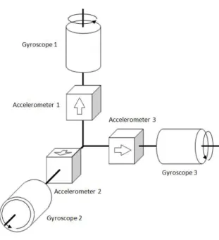
In Inertial Navigation Systems the rotation matrixes, also known as cosines matrixes, have an important role once that they allow the transformation of vector’s components from one coordinate system to another one. The utilization of this kind of matrixes on inertial systems is due to the need to transform vector components from sensor’s axis system to an earth fixed axis system. The following equations shows the construction processo of one of these matrixes in a two dimensional frame.

In Figure 3.5 there is P vector which represents the vector to be transformed to a new referential and has as original referential X1,Y1 with an inclination angle . The rotation angle between the two frames it is represented by ψ and P’ represents the P vector transformed from referential X1 ,Y1 to the coordinate system X2 ,Y2.

23

Using and ψ angles it is possible to obtain the P vector projections in X1,Y1 and the P’ projections in X2 ,Y2:

P5= L ∙ cos(α)

P;= L ∙ sin(α)

P′5= L ∙ cos(α + ψ)

P′;= L ∙ sin(α + ψ)

Through Euler’s formula it is possible to represent the addition of angles as follows:

cos(x + y) = cos(x) ∙ cos(y) − sin(x) ∙ sin(y) sin(x + y) = cos(y) ∙ sin(x) + cos(x) ∙ sin(y)

Using the previous expressions and P and P’ vectors’ projections in the respective coordinate systems:

P′5= L ∙ cos(α) ∙ cos(ψ) − L ∙ sin(α) ∙ sin(ψ)

P′;= L ∙ cos(ψ) ∙ sin(α) + L ∙ cos(α) ∙ sin(ψ)

P′5= P5∙ cos(ψ) − P;∙ sin(ψ)

P′;= P5∙ sin(ψ) + P;∙ cos(ψ)

If the two previous equations be placed in matrix form, we have

P′ = C_P′P′5

;D = Ecos(ψ) − sin(ψ)sin(ψ) cos(ψ) F ∙ E

P5

P;F

this is, to obtain P’ projections from P, it is multiplied the component’s vector by transformation matrix.

P′ = C ∙ P

Though, C is the transformation matrix

C = Ecos(ψ) − sin(ψ)_{sin(ψ) cos(ψ) F}

Considering the right hand rule and a three axes frame, once we have a rotation with a angle ψ in the Z axis, the matrix could be re-written in the following form

RIH= J

cos(ψ) − sin(ψ) 0 sin(ψ) cos(ψ) 0

0 0 1M

24 Z Rotation

Jx′y′ z′M = J

cos(ψ) − sin(ψ) 0 sin(ψ) cos(ψ) 0

0 0 1M ∙ C x y zD

Y Rotation

Jx′y′ z′M = J

cos(θ) 0 − sin(θ)

0 1 0

sin(θ) 0 cos(θ) M ∙ C x y zD

X Rotation

Jx′y′ z′M = J

1 0 0

0 cos(ϕ) sin(ϕ) 0 − sin(ϕ) cos(ϕ)M ∙ C

x y zD

Combining all three possible rotations on the three different axes, each one with respective rotation angle, the following equations can be used

C = RHI ∙ RRQ∙ RST

C = Jcos(ψ) − sin(ψ) 0sin(ψ) cos(ψ) 0 0 0 1M ∙ J

cos(θ) 0 − sin(θ)

0 1 0

sin(θ) 0 cos(θ) M ∙ J

1 0 0

0 cos(ϕ) sin(ϕ) 0 − sin(ϕ) cos(ϕ)M

C = Jcos θ cos ψ sin ϕ sin θ cos ψ − cos ϕ sin ψ cos ϕ sin θ cos ψ + sin ϕ sin ψcos θ sin ψ sin ϕ sin θ sin ψ + cos ϕ cos ψ cos ϕ sin θ sin ψ − sin ϕ cos ψ

− sin θ sin ϕ cos θ cos ϕ cos θ M

Figure 3.6 - Rotation over Z axis

Figure 3.7 - Rotation over Y axis

25

3.2.2

NED/ECEF and ENU/ECEF Transformations

Figure 3.9 - Representation of NED coordinate system on ECEF

In applications involving inertial navigation it is, normally, used NED system which coincides with RPY (Figure 3.4) system when vehicle is facing. In this kind of applications, the use of ENU systems is also common. So, it is needed a transformation between the Local Tangent Plane used and a frame like ECEF to have the platform’s position in Earth. These transformations are obtained through rotation matrixes using latitude (L) and longitude ( ).

The following equations show the transform matrixes between ECEF and NED systems:

= Jcos U − sin U 0sin U cos U 0 0 0 1M ∙ J

cos V 0 − sin V

0 1 0

sin V 0 cos V M ∙ J

0 0 −1 0 1 0 1 0 0 M,

= J−cos U ∙ sin V −sin U −cos U ∙ cos V−sin U ∙ sin V cos U −sin U ∙ cos V cos V 0 − sin V M

= J− cos U ∙ sin V − sin U ∙ sin V cos V− sin U cos U 0 − cos U ∙ cos V −sin U ∙ cos V − sin VM

Once that transformation matrix from NED to ENU and ENU to NED could be represented by W₌

W = J

26

the ECEF/ENU transformation can be computed in a similar way as ECEF/NED or computed from it. This is, the _W is result of multiplying the matrix W by :

W = W ∙ = J

0 1 0 1 0 0 0 0 −1M ∙ J

−cos U ∙ sin V −sin U −cos U ∙ cos V −sin U ∙ sin V cos U −sin U ∙ cos V cos V 0 − sin V M

W = J

−sin U −cos U ∙ sin V cos U ∙ cos V cos U −sin U ∙ sin V sin U ∙ cos V

0 cos V sin V M

W _{= J−cos U ∙ sin V −sin U ∙ sin V cos V}−sin U cos U 0

cos U ∙ cos V sin U ∙ cos V sin VM

3.2.3

Transformation between ECEF and ECI

ECEF and ECI coordinate systems are very similar. As the Figure 3.2 shows, the only difference is that in ECEF system the x axis is pointing to the Greenwich meridian while the x axis of ECI is pointing to the local meridian. So, to transform coordinates of one system to another only the longitude has to be considered. These transformations are a single rotation over the z axis (which is common to both systems).

The transform from ECI to ECEF and ECEF to ECI are represented by the following matrixes respectively:

= Jcos U −sin U 0sin U cos U 0

0 0 1M = J

cos U sin U 0 −sin U cos U 0

27

3.3

Navigation Equations

Navigation equations are used, generally, in inertial navigations systems to know a body’s localization with a respect to a fixed frame. The following explanation is based on Titterton [Titterton, 2004].

By Newton’s second law of motion it is known that a body under a specific force will accelerate. The acceleration of a generic point in an inertial frame is given by:

X

Y

= Z

[

\

_]

[^

\

_

Y

(3.1)

Assuming that we have accelerometers in the three axes providing the specific force (f) at the body:

` = Z

[

_[^

\

]

_\

_

Y

− a

(3.2)

Note that gravitational force (g) is always present (once we consider that the body is in the Earth) and its effect is always measured by accelerometers.

Rearranging the Equation (3.2) and taking in consideration Equation (3.1) it is quite noticeable that the acceleration measured contains the specific force and gravitational force.

Z[

\

]

[^

\

_

Y

= ` + a

(3.3)

Equation (3.3) can be considered a navigation equation once that it is possible to obtain quantities of velocity and position by integration. So, the first integral of the acceleration gives the velocity and the second integral gives the position.

b

Y

Z= []

_[^c

Y

(3.4)

28

velocity of the body over an inertial frame and a fixed frame. Therefore, a frame fixed to the Earth is needed and Earth’s rotational velocity must be considered.

In Equation (3.5) b_d can be obtained from the inertial velocity (Equation (3.4)) using the theorem of Coriolis:

bdZ= []_[^c

d= bY− eYd⨂]

(3.5)

The rotational velocity of the Earth with respect to an inertial frame is represented by e_Yd=

gh h ijk_.

Combining Equations (3.4) and (3.5) in order to translate the velocity from a fixed frame to a inertial frame. This is, computing the inertial velocity from the ground speed and Coriolis equation, we have:

ZZ[] [^cY=

[]

[^c_d+ eYd⨂] (3.6)

Differentiating this expression and writing Z l = m ,

ZZ[\] [^\_

Y =

[bd

[^ __Y+ Z[^ ge[ Yd⨂]jcY

(3.7)

Applying the Coriolis equation in the form of Equation (3.6) to the second term in Equation (3.7), we have

ZZ[\] [^\_

Y =

[bd

[^ __Y+ eYd⨂bd+ Z[^ ge[ Yd⨂]jcY+ eYd⨂geYd⨂]j

(3.8)

where _[^[e_Yd= 0, once it’s assumed that the turn rate of Earth is constant. The previous equation can be simplified:

ZZ[\] [^\_

Y =

[bd

[^ __Y+ eYd⨂bd+ eYd⨂geYd⨂]j (3.9)

29

Z` + a = [bd

[^ cY+ eYd⨂bd+ eYd⨂geYd⨂]j

(3.10)

Z[bd

[^ cY = ` − eYd⨂bd− eYd⨂geYd⨂]j + a

(3.11)

In this equation, f represents the specific force of the acceleration acting on the body, the term

eYd⨂bd is the Coriolis acceleration which is the acceleration caused by body’s velocity over the surface of the rotating Earth, e_Yd⨂ge_Yd⨂]j is the centripetal acceleration (also caused by the rotational velocity) and it is not distinguishable from the gravitational acceleration g. The sum of these two last terms (centripetal force and gravitational force) is also known as local gravity vector. It takes the symbol g1and could be represented by:

a

n

= a − e

Yd

⨂ge

Yd

⨂]j

(3.12)

Figure 3.10 - Diagram showing the components of the gravitational field [Titterton, 2004]

3.3.1

Earth frame mechanization

30

ZZ[bd

[^ cd=

[bd

[^ c_Y− eYd⨂bd (3.13)

Merging the (3.11), (3.12) and (3.13), we have:

Z[bd

[^ cd= ` − 2eYd⨂bd+ an

(3.14)

3.3.2

Local frame mechanization

In a similar way of Earth frame mechanization, the ground speed in local frame (as NED) it is obtained from ground speed in inertial frame (from Equation (3.11)). To do this, it’s necessary to consider the turn rate of the Earth plus the turn rate of the local geographic frame with respect to the Earth-fixed frame. The following equation describes the

ZZ[bd

[^ co=

[bd

[^ c_Y− geYd+ edoj⨂bd (3.15)

Merging the (3.11), (3.12) and (3.15), we have

Z[bd

[^ co= ` − 2geYd+ edoj⨂bd+ an

31

3.4

Strapdown Inertial Navigation Systems

Considering Newton’s laws of motion (especially the 1st) that says that a body will move in uniform movement in a straight line or stay still in its state of rest unless it has a force impressed on it. Newton’s second law tells us that a force over a body will produce a proportional acceleration of the body. So, to mathematically be able to obtain velocity and position by successive integration it is needed the acceleration, which can be obtained from accelerometers. Gyroscopes and magnetometers are, also, useful instruments to perceive body’s orientation and, thus, to do inertial navigation.

A strapdown inertial navigation system is composed by sets of these instruments in the three different axes. Some authors refer to these systems as: “A strapdown inertial navigation system is basically formed from a set of inertial instruments and a computer” [Titterton, 2004]. Walchko and Mason says that a “strapdown system is a major hardware simplification of the old gimbaled system” [Walchko and Mason, 2002].

The main difference between inertial navigation systems and other types of navigation systems is that inertial systems are entirely self-contained within a vehicle and, for that reason, they do not depend on signal transmission from the vehicle to a base station where decisions due to navigation could, eventually, be taken. However, because of that absence of communication, this kind of systems only can be used to obtain a relative estimation of position. To estimate the body’s localization in the earth it will depend on an accurate knowledge of vehicle’s position at the start of navigation.

With the development of the technology that provided advances in sensing technology, appeared different implementations of strapdown systems. Nevertheless, the purpose and principles of operation are the same. In the original applications of inertial systems the inertial sensors are mounted on a stable platform and are mechanical isolated from the rotational motion of vehicle. Although its size and weight, this approach is still used, particularly for those who need a very accurate data as submarines and ships [Titterton, 2004].

Figure 3.11 - Orthogonal instru

The instrument cluster and the in Measurement Unit). Combining computation we have an AHRS Navigation System is the result o as illustrated in Figure 3.12.

Figure 3.12 - Inertial Nav

Inertial Navigatio

Navigation Equations

Atit

At Com 32

rument cluster arrangement, adapted from Titterton [T

instrument electronics combined together is called g the information obtained in IMU with a proces S (Attitude and Heading Reference System). Fin t of combining an AHRS with the Navigation Equ

avigation System representation, adapted from Titterto 2004]

ation System

Atittude and Heading Reference System (AHR

Atittude Computation

Inertial Measurement Unit (IMU

Accelerometers Gyroscopes Magnetomet

[Titterton, 2004]

led an IMU (Inertial essor to do attitude Finally, the Inertial quations Computing

ton [Titterton,

(AHRS)

IMU)

33

3.5

Kalman Filter

The Kalman filter is a mathematical method introduced by Rudolf Kalman in 1960. In [Kalman, 1960], Kalman formulates and solves the Wiener problem and introduces the Kalman filter as it is known today. Since then, many generalizations and extensions were developed and, thus, making this method one tool used in many applications to estimate the true state of a system. According to Welch and Bishop [Welch, 2006], the area of autonomous or assisted navigation was one of the most responsible for the study and research that led to generalizations and extensions mentioned before.

Maybeck describes the filter as a “(…) simply an optimal recursive data processing algorithm.” [Maybeck, 1979]. In this method, it is possible to add any information that is available to estimate the true state of the system. This means that Kalman Filter processes all available measurements regardless of their precision in order to estimate the current value of the variables of interest. To estimate variable’s state the Kalman filter uses its knowledge of system and measurement device dynamics, the statistical description of noises, measurement errors and uncertainly in the dynamic models and also takes in account all possible available information of initial values of variables of interest.

The following explanation of Kalman filter is based on the one given by Welch [Welch, 2006]. The state of the system is a vector x with n variables which describe interesting characteristics of the system. To estimate the state of system, p ∈ ℜ , the Kalman filter uses the linear stochastic2 difference equation:

s

t = u

s

tvn + wxt + yt−n (3.17)

In linear stochastic equation (3.17) there are matrices A and B. The matrix A is a × matrix designed as state transition matrix and represents the state evolution over time. This is, this matrix relates the state at { − 1 with the state at {. B is known as control matrix, is a × | matrix and relates the control input, & ∈ ℜ}, with the state x.

The measurement is represented by

z

_~ ∈ ℜ•

2

34

€

t = •

s

t + bt (3.18)

In (3.18), the true measurement ‚_' ∈ ℜƒ at time k depends linearly on the state of system p_'. The H matrix is used to relate the state p_'

with the measurement

‚_'

. This means, given a state the,

H tells what the real measurement should be with no errors. However, once those measurements are obtained through sensors they are noisy and this noise is modeled by m_' ∈ ℜƒ.

The random variables y_t and b_t represent, respectively, process and measurement noise. It’s assumed that they are independent, white and with normal distributions and are represented by:

(„)~†(0, ) (m)~†(0, )

where Q and R represents, respectively, process noise covariance and measurement noise covariance.

3.5.1

Computational Consideration

The a priori estimate of the estate at step k is represented by s‡_tv, where the ‘^’ denotes that is an estimate, ‘-’ denotes that is a priori and ‘k’ identifies the step of process the value belongs. s‡_t represents the a posteriori estimate of the system current state. Negenborn refers to a priori and a posteriori estimates as beliefs [Negenborn, 2003]. In his work, s‡_tv is also referred as the prior belief ( "|v(p_')) which represents the belief about system’s state after incorporating all information up to step k, including the last relative measurement but non including the absolute measurement z_~ in step k. The a posteriori estimate corresponds to the posteriori belief ( "|(p_')) and represents the belief about system’s state after has included the absolute measurement

The error of a priori estimate and a posteriori estimate could be represented, respectively, as:

"'v≡ p'− p‰'v

"' ≡ p'− p‰' System

Kalman Filter

€

t

s‡

t

35

Thus, we have the a priori estimate error covariance and a posteriori estimateerror covariance:

'v≡ Šg"'v"'v,j

' = Šg"'"',j

These covariance matrices reflect the uncertainty level in the respective estimates of the current state.

In the Kalman filter, an a posteriori estimate of system’s state is represented by the following equation:

p‰' = p‰'v+ ‹'(‚'− Œp‰'v) (3.19)

The difference (‚_'− Œp‰_'v) is called measurement innovation. This matrix expresses the discrepancy between the predicted measurement Œp‰_'v and the actual measurement ‚_'. This matrix also can be called residual and if it takes a zero value it means that predicted state is equal to the measured.

Returning to equation (3.19), the a priori estimate of state is a combination of the system’s state obtained in the previous step (k-1) and

the

difference referred before weighted by ‹_', Kalman gain matrix – Equation (3.20). This matrix minimizes the a posteriori error covariance when used in (3.19) once it aims to reduce the difference between the a posteriori state estimate (computed in (3.19)) and the true state of system. One of the more popular forms to represent this matrix is presented by the following equation:

‹'= 'vŒ,(Œ 'vŒ,+ )vŽ (3.20)

3.5.2

Kalman Filter Algorithm