Abstract— The importance of assembly areas for enterprises producing in countries with high wages increases steadily against the background of global competition. This article describes an approach for modeling logistic assembly processes with respect to enhancing an extensive theory of logistics. The models described in this article are intended to support the economical organization and logistic control of assembly processes.
Index Terms— Logistics and Supply Chain, Production and Operation Management, Assembly Logistics, Theory of Logistics.
I. INTRODUCTION
The strategic significance of logistic efficiency is undisputed [1] – [3]. Logistic objectives such as delivery reliability and delivery time are thus taking on more critical roles in global competition [4], [5]. This explains the enormous upsurge in logistics, which has developed into an economically noteworthy economical area in countries with high wages such as Germany [6]. At the same time, the significance, range and complexity of logistics has grown quicker than the hypotheses and theories needed to describe them. Supporting logistics with a theoretical-methodical foundation is, therefore, increasingly important. In particular developing more comprehensive models for describing cause and effect relationships as well as for supporting decision making becomes more pertinent [7]. The key position of assembly in fulfilling customer demands regarding delivery reliability and delivery time and for economically designing production processes is illustrated by the large portion of manufacturing time dedicated to assembly. Depending on the sector and product, assembly time accounts for anywhere from 15 to 70% of the entire manufacturing time [8], [9].
In the order fulfillment process, assembly occurs after the construction, material planning, procurement, preparation and manufacturing. Errors or disruptions appearing in these
Manuscript received July 1, 2008.
Matthias Schmidt is with the Institute of Production Systems and Logistics at the Leibniz University of Hannover, An der Universitaet 2, D-30823 Garbsen, Germany (phone: +49-511-762-18130; fax: +49-511-762-3814; e-mail: [email protected]).
Daniel Berkholz is with the Institute of Production Systems and Logistics at the Leibniz University of Hannover, An der Universitaet 2, D-30823 Garbsen, Germany (e-mail: [email protected]).
Peter Nyhuis has been appointed both as a professor for Production Systems, Logistics and Work Sciences as well as the director of the Institute of Production Systems and Logistics at the Leibniz University of Hannover, An der Universitaet 2, 30823 Garbsen, Germany (e-mail: [email protected]).
processes have a greater probability of causing throughput time relevant and critical scheduling deviations in the assembly. With regards to the causes of assembly disruptions, an analysis of 14 assembly areas from various mechanical engineering enterprises shows that the roots of over 91% of disruptions can found in material shortages due to upstream assembly processes. Of these, a large portion can be traced back to logistic deficiencies such as missing parts or supplying incorrect parts [10], [11]. One option for countering these shortcomings is to maintain a high safety stock level in the stores or allocation area. Nowadays, from an economics viewpoint however, this approach is no longer justifiable in assemblies due to the high capital tie-up costs, the risk of having to scrap parts, and the increasing processing costs [12]. A model based description of the logistic operations in an assembly process is an elementary prerequisite for making this field of tension and the prevailing complexity controllable.
II. CURRENT STATE OF RESEARCH
The allocation or provision process joins the material supply to the assembly. Among other tasks, the job of allocations is to provide the assembly with the necessary materials according to type, quantity and time. Supplying the assembly is often characterized by a high level of complexity: Materials for assembly can be received from the enterprise’s own manufacturing, from a warehouse or directly from a supplier. In the following section, we will introduce various models which have been implemented for describing assembly and provision processes.
A. Modeling of Assembly Processes
In addition to mathematic models based purely on random parameters which are commonly applied in optimizing economical systems such as discrete part manufacturing, assembly and material provision [13], there are descriptive approaches for modeling the production logistics of assembly processes. The most common of these are network planning, assembly priority charts and Gantt diagrams.
Today, assembly processes are frequently modeled with the assistance of methods used in project management. Thus for example network planning is applied in order to visually represent the sequence of assembly processes and their logical relationships. Network planning provides support for determining the schedule of interconnected assembly orders, describing the processes and their dependencies either through graphs or tables. According to DIN 69900-1 the term network planning comprises “all methods for analyzing, describing, planning, controlling and monitoring processes
Modeling of Logistic Processes
in Assembly Areas
based on graph theory, whereby time, costs, or resources can be taken into consideration” [14]. The goal of network planning in depicting the interconnected assembly orders is to coordinate the logistic processes as they occur in the assembly, for example, when the supply processes are coordinated with the assembly’s demand date.
Depending on the degree of the network planning detail, different descriptive models can be derived from it. The assembly priority chart is a simple representation similar to network planning. It illustrates the sequence of the assembly processes and the resulting relationships [15]. The priority chart is thus frequently implemented for visualizing the organization of the assembly processes. Depending on the level of observation, dependencies between the individual sub-tasks in the work schedule or the entire assembly and supply operations can be represented.
In contrast to network planning the Gantt diagram visualizes the chronological sequence of operations in the form of bars over a time axis. The duration of an assembly operation is explicitly represented and visually comprehensible in the length of the respective bar. Here too, critical paths and buffer times can be graphically depicted [11]. However, the Gantt diagram is only able to limitedly describe the dependencies between the operations.
B. Throughput Diagram and Logistic Operating Curves The work described in this paper is based on models developed at the Institute of Production Systems and Logistics. The starting point for the development was the definition of a basic production logistics element – the throughput element. On the logistic processes level, the throughput element defines the throughput time of one operation as the time one order requires from the end of the previous operation, or as it may be, the point of the order input (i.e., with the first operation) until the end of the observed operation. When the manufacturing is completed in lots an order will be transported to the subsequent workstation after the completion of an operation and possible waiting time at the corresponding station. Once at the next workstation, the lot usually meets another queue and has to wait until the orders to be completed ahead of it are processed. Provided the capacities required to handle the order are available, the workstation can be reset and the processing of the lot can be carried out [16].
The throughput element also forms the basis for the
100 300 500 700
170 190 210 230
w
o
rk
content
[hrs]
Work in Process
Output Curve
Input Curve
shop calendar days (SCD) [-] Fig. 1: Throughput Diagram.
mean work in process [hrs]
0 10 20 30
0,2 0,6 1,0 1,4 1,8 actual operating point target operating point
0 4 8 12
m
ean o
u
tp
ut rate [hrs/
S
CD]
m
e
a
n
th
ro
ug
hp
u
t ti
m
e
[S
C
D
]
Throughput Time Curve
Output Rate Curve
Fig. 2: Logistic Operating Curves.
throughput diagram as a descriptive model (Fig. 1). In this, the input and output on a workstation are cumulatively plotted over the time. This allows the dynamic system behavior to not only be described accurately and comprehensively both qualitatively and chronologically, but also allows key performance figures (e.g., WIP and output rate) to be read. The throughput diagram offers a reliable approach for analyzing and interpreting the logistic behavior of the observed work system.
The output curve shows the outgoing orders’ accumulated work content during the investigation period. Since it has a constant slope, the workstation’s output rate reveals no significant fluctuations. The input curve visualizes the accumulated work content of the incoming orders. Its slope indicates certain fluctuations, which can be traced back to the workstation’s varying load. The WIP level on the workstation, therefore, also oscillates as it results from the difference between the in- and output.
The throughput diagram and the key figures derived from it each describe a specific stationary operating state. These operating states can be strongly aggregated into the form of an impact model referred to as logistic operating curves (LOC). In order to accomplish this each of the values for the output rate and range are plotted as a function of the WIP. Fig. 2 illustrates the LOC for an exemplary work system (in this case a resist coating workstation). The Output Rate Operating Curve (OROC) indicates that the output rate of a workstation changes only negligibly above a certain WIP level. From this point on, there is continuously enough work available to ensure that there are no WIP dependent breaks in production. The range (and therefore also the throughput time) in contrast, generally increases above this critical level proportional to the WIP [16].
We can see that the calculated operating point is located well into the overload operating zone and that there is a high WIP level on the workstation. The output rate is therefore high, but there are also long throughput times. Reducing the WIP by approximately 20 hours would make it possible to reduce the throughput time by approximately 75%, without notable output rate losses.
Des c ri pti v e Mod e l Im p a c t Mo d e l Procure-ment As-sembly Distri-bution Warehouse Distri-bution Transport Manufac-turing [Kuhn] [Kuhn] Des c ri pti v e Mod e l Im p a c t Mo d e l Procure-ment As-sembly Distri-bution Warehouse Distri-bution Transport Manufac-turing [Kuhn] [Kuhn] [Kuhn] [Kuhn]
Fig. 3: Developments Attained on the Way to a Logistic Theory
theory”. The current state of developments in descriptive and impact models is outlined in Fig. 3. While these models already exist for production [16], stores [17] and transportation [18] (generally in the form of throughput diagrams and logistic operating curves), they are still being developed for assembly.
Current work is focused on developing so-called ‘allocation diagrams’ for multi-level products. These diagrams depict how the due date behavior of the upstream processes and in particular their synchronization, impact the WIP and delivery reliability situations in the assembly [19].
III. ASSEMBLY THROUGHPUT ELEMENT – THE FINITE
ELEMENT OF ASSEMBLY LOGISTICS
Similar to production logistics; the logistic assembly processes which are to be described can be differentiated from the perspectives of both orders and resources (Fig. 4). The order perspective describes the chronological throughput of individual orders through the enterprise’s assembly. The approaches outlines in section 2.1 are focused on this view. The order’s throughput can be described in simplified terms by lining-up various operations and assembly processes which can be represented with production or assembly throughput elements.
Resource View (Assembly
System 3) WS : Work System
AS : Assembly System OP: Operation
AP : Assembly Process WS : Work System
AS : Assembly System OP: Operation
AP : Assembly Process
Order View (order A) AP1 AS3
OP3 WS5 OP4 WS7 OP2 WS2 OP1 WS1
AP1 AS3
OP3 WS1 OP4 WS4 OP2 WS3 OP1 WS1
OP1 WS1 OP2 WS2
AP1 AS3
OP5 WS1 OP6 WS3 OP4 WS7 OP3 WS5 AP1 AS3 AP2 AS3 AP3 WS5 OP5 WS9
Fig. 4: Resource and Order Related Views of an Assembly
The resource view in contrast, describes the completion behavior of the assembly orders on a single assembly system. It thus includes a number of assembly operations for different orders. Suitable approaches for modeling this perspective in order to comprehensively describe logistic processes in the assembly are not currently available.
Analogous to the production throughput element the assembly throughput element forms the basis for describing logistic operations in an assembly process. It thus combines the order and resource views (cf. Fig. 4). An example of an assembly throughput element is shown in Fig. 5, whereby the assembly order here consists exemplarily of three supply orders. A supply order starts after the completion of the upstream process and runs through the basic elements “waiting time after upstream process”, “transport” and “waiting time before assembly” up until the “setup” is conducted on the assembly system and the “assembly” can begin.
The “waiting time after upstream process” describes the time period during which a supply order is awaiting transport to the assembly system after a preceding process or operation has been completed. “Transportation” describes the period of time required for the physical transport of a lot or work piece from a preceding process to the assembly system. The “waiting time before assembly” refers to the period in which the supply order is awaiting the start of the actual assembly process.
As is depicted in Fig. 5, key scheduling and time figures can be derived from the one dimensional assembly throughput element. The assembly throughput element of an assembly order starts with the end of the first supply order’s preceding process. The time up until the start of the setup is defined as the interoperation time, whereby the interoperation time can be divided into disrupted time and time in which an order competes for capacity on an assembly system. During the disrupted time, the assembly order cannot
Waiting After Processing Transportation
Assembly
Setup Waiting Before Assembly
time [SCD] AED ASD FPDPP LPDPP TOP TIO DT TTP TCC
ASD: Assembly Start Date [SCD]
SCD: Shop Calendar Day Assembly End Date [SCD] AED:
Operation Time [SCD] TOP:
Interoperation Time [SCD] TIO:
Throughput Time [SCD] TTP:
Disrupted Time [SCD] DT:
FPDPP:First Processing Date of Preceding Process [SCD]
LPDPP:Last Processing Date of Preceding Process [SCD]
Time during which Order Competes for Capacity [SCD] TCC:
Waiting After Processing Transportation Waiting After Processing
Waiting After Processing TransportationTransportation
Assembly Assembly
Setup Waiting Before Assembly SetupSetup Waiting Before Assembly
Waiting Before Assembly
time [SCD] AED ASD FPDPP LPDPP TOP TIO DT TTP TCC
ASD: Assembly Start Date [SCD] ASD: Assembly Start Date [SCD]
SCD: Shop Calendar Day SCD: Shop Calendar Day
Assembly End Date [SCD] AED: Assembly End Date [SCD] AED:
Operation Time [SCD] TOP: Operation Time [SCD] TOP:
Interoperation Time [SCD] TIO: Interoperation Time [SCD] TIO:
Throughput Time [SCD] TTP: Throughput Time [SCD] TTP:
Disrupted Time [SCD] DT: Disrupted Time [SCD] DT:
FPDPP:First Processing Date of Preceding Process [SCD] FPDPP:First Processing Date of Preceding Process [SCD]
LPDPP:Last Processing Date of Preceding Process [SCD] LPDPP:Last Processing Date of Preceding Process [SCD]
Time during which Order Competes for Capacity [SCD] TCC: Time during which Order Competes for Capacity [SCD] TCC:
be processed because not all of the supply orders necessary for the assembly are available. This is only the case after the chronologically last processing deadline of a previous process. After this point in time the assembly order is completed and can be processed, it thus competes for capacity on the assembly system.
This definition was chosen in order to meet the requirements found in the industrial practice where feedback is generally available for work operations, however, not for the start and end of the transport. Should the data be available it is clearly possible to separately identify all portions of the interoperation time. Similar to the production throughput time element, the operation time, which together with the interoperation time describes the throughput time, consists of the setup time and the processing time – that is the assembly time.
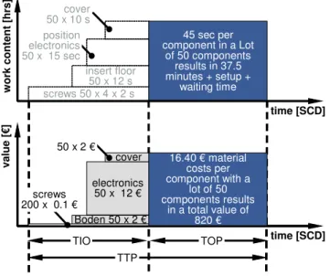
In order to now evaluate the individual throughput elements which can be processed on an assembly system, they have to be provided with a second dimension (Fig. 6). In the upper portion of the figure, the work content of the assembly order is selected as the second dimension. It is necessary to consider the work content so that the WIP on an assembly system can be laid out with consideration to the desired utilization and targeted throughput time (cf. [16]).
Similar to the one dimensional assembly throughput element, the different supply orders are logged out of upstream processes at different points in time. Whereas the assembly order’s total work content can be drawn from the work schedule, it cannot be easily allocated to the individual supply orders. Various approaches for doing so can be found in other studies (cf. [20]). However, only the work content of the assembly order and not the supply orders is relevant later when considering the assembly system’s utilization. This is because only a complete order that can compete for capacities can contribute to the utilization of an assembly system. Assigning the work content to various product components can therefore be ignored.
In the value oriented analysis of the supply orders, found in the lower portion of Fig. 6, the differentiation of the individual orders is of interest. The value of an input supply order is known (e.g., the replacement cost of a store article)
insert floor 50 x 12 s screws 50 x 4 x 2 s
45 sec per component in a Lot
of 50 components results in 37.5 minutes + setup +
waiting time
time [SCD]
w
ork
conte
n
t [hrs
]
Boden 50 x 2 € electronics
50 x 12 €
cover 16.40 € material costs per component with a
lot of 50 components results
in a total value of 820 €
time [SCD] TOP
TIO
TTP
va
lue [
€
]
50 x 2 €
screws 200 x 0.1 €
position electronics 50 x 15 sec
cover 50 x 10 s
Fig. 6: Two Dimensional Assembly Throughput Element
and can thus be drawn upon for determining the exact capital tie-up costs on a work system. The sum of the values of all the input supply orders is the value of the assembly order. The value adding which occurs on the assembly system will initially not be considered here.
IV. ASSEMBLY THROUGHPUT DIAGRAM
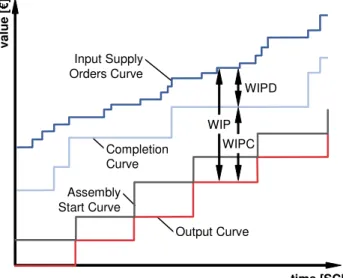
By plotting a number of these two dimensional throughput elements over the time in a graph, an assembly throughput diagram results. An assembly throughput diagram is a descriptive model from the perspective of resources. Fig. 7 depicts an example of such a diagram, whereby the value of the supply and assembly orders is selected as the second dimension for illustrative purposes.
The output (red curve) specifies the cumulative output of all orders on the assembly system over time. It thus documents the output rate on the system. The graph of the assembly’s start (gray curve) shows the starts of each orders’ processing, whereby the processing consists of both the setup and assembly. The completion curve (light blue) cumulatively describes over time when an assembly order on the assembly system is completed via the corresponding supply orders. From this point on the described order competes for capacity on the assembly system. The input of supply orders on the assembly system is expressed by the input curve (dark blue). The input of individual supply orders on the assembly system cannot ensure the utilization of the system, since only completed assembly orders can be processed.
Various key figures can be derived from the assembly throughput diagram. As an example a number of WIP related figures are depicted here. The amount of supply orders for uncompleted assembly orders forms the disrupted WIP on the assembly system (vertical distance between the input curve and the completion curve). The vertical distance between the completion curve and the output curve at a specifically observed point in time describes the WIP for the completed assembly orders. The sum of the disrupted WIP and the completed assembly orders WIP is the assembly system’s existing WIP.
The curves depicted in Fig. 7 cumulatively plot the events on an assembly system over the time. Therefore the assembly throughput elements introduced in section 3 cannot be directly read from this diagram. Nonetheless the elements do form the theoretical foundation for the assembly throughput diagram. It is also possible to organize it according to throughput elements and thus open further possibilities for interpreting, for example, by considering the surface areas of the elements.
Examining the ideal versions of the described curves allows additional key figures such as the mean throughput time on an assembly system or the mean duration required to complete an order, to be determined. An example of an ideal assembly throughput diagram is depicted in Fig. 8. The ideal curves are derived by connecting the initial and final points of the output, assembly start, completion or input curves.
Assembly Start Curve
WIPD : Disrupted WIP [€] WIPD : Disrupted WIP [€]
WIP Completed and Competing for Capacity [€] WIPC : WIP Completed and Competing for Capacity [€] WIPC :
time [SCD]
val
ue
[€]
WIPD
WIPC WIP
Work in Process [€] WIP : Work in Process [€] WIP :
Input Supply Orders Curve
Output Curve Completion
Curve
Fig. 7: Value Related Assembly Throughput Diagram
assembly order’s first input and the order’s completion. The horizontal distance between the ideal completion and assembly start curves represents the average length of time an order competes for capacities on an assembly system. The mean interoperation time is equal to the sum of both time periods. The horizontal distance between the ideal assembly start curve and the output curve describes the mean operation time. The mean operation time and the mean interoperation time result in the mean throughput time on the assembly system.
The vertical distance between the ideal input and completion curve forms the mean disrupted WIP on the observed assembly system. This WIP cannot be processed since it is waiting to be completed. The vertical distance
between the ideal completion curve and the output curve describes the mean completed WIP, i.e., the WIP which is competing for capacity on the assembly system. The mean WIP on the assembly system is equal to the sum of both these WIP figures (vertical distance between the ideal input and output curves). The rate of completed assembly orders can be determined from the ratio of the mean completed WIP to the mean WIP on the assembly system. This is a measure of the logistic quality of the assembly system’s supply. The higher the completion rate the better synchronized – that is the more punctual – the supply orders on the assembly system are allocated (cf. [19]).
The vertical distance between the ideal input and output curves at the beginning and end of an observation period describes the initial and final WIP on the assembly system. The output on a system in relation to the observation period defines the assembly system’s mean output rate. This corresponds to the slope of the ideal output curve. The slope of the ideal completion curve describes the load of the capacity unit, i.e., the assembly system.
The model outlined here for describing the logistic processes in the assembly area aids the analysis of these processes in both provisions and assembly. The assembly throughput diagram makes it possible to clearly depict the converging material flow in the assembly as well as to derive the logistic and economic related key figures. The assembly throughput diagram thus provides support for evaluating the quality of the process.
The basis of the chronologically discrete description in assembly throughput elements is formed by operational data which can generally be compiled with the help of an operational data recording system. The assembly throughput diagram together with the possible applications outlined here provides support in deriving measures for improving logistic processes and increasing the economic efficiency of the assembly area.
Ideal Assembly Start Curve
WIPDm
WIPCm
WIPm
Out
put
d
uri
ng
Obs
ervat
ion P
eri
o
d
time [SCD]
val
u
e [€]
TTPm DTm
TOPm TIOm
TCCm
Observation Period
In
itia
l W
IP
F
inal
W
IP
ROUTm MLm
Input
d
uri
ng
Obs
ervat
ion P
eri
o
d
Mean Operation Time [SCD] TOPm: Mean Operation Time [SCD] TOPm:
Mean Throughput Time [SCD] TTPm: Mean Throughput Time [SCD] TTPm:
Mean Interoperation Time [SCD] TIOm: Mean Interoperation Time [SCD] TIOm:
Mean Time during which Order Competes for Capacity [SCD] TCCm: Mean Time during which Order
Competes for Capacity [SCD] TCCm:
Ideal Input Supply Orders Curve
Ideal Output Curve
Ideal Completion Curve
Fig. 8: Value Oriented Assembly Throughput Diagram
Mean Disrupted Time [SCD] DTm: Mean Disrupted Time [SCD] DTm:
Mean WIP of Completed Assembly Orders [€] WIPCm: Mean WIP of Completed
Assembly Orders [€] WIPCm:
Mean WIP [€] WIPm: Mean WIP [€] WIPm:
Mean Disrupted WIP [€] WIPDm: Mean Disrupted WIP [€] WIPDm:
Mean Load [€/SCD] MLm: Mean Load [€/SCD] MLm:
V. CONCLUSIONS
Logistics strongly influence the economically significant assembly areas in numerous industrial enterprises because a large proportion of disruptions in assembly processes are caused by insufficient logistics. Besides various planning tools there are no sufficient models for describing the chronological logistic behavior of an assembly system. The assembly throughput diagram, which is based upon the assembly throughput element, delivers a very promising approach for doing so. It offers numerous possibilities for interpreting the logistic behavior and for deriving key logistic figures from assembly systems. A few of these possibilities have been introduced here.
Extensive research at IFA is currently focused on the detailed realization of the model outlined here, whereby the general validity of the developed model is ensured for the various organizational forms of the assembly (workstation assembly, continuous assembly lines etc.). These models have to be validated in the industry setting and methods for deriving improvement measures have to be developed.
REFERENCES
[1] B. Enslow, Best Practices in International Logistics. Benchmark
Report. Boston: Aberdeen Group, 2006.
[2] J. H. Kim and N. A. Duffie, "Design and Analysis of Closed-Loop Capacity Control for a Multi-Workstation Production System," in
Annals of the CIRP, vol. 54, no. 1, 2005, pp. 455-458.
[3] H. Wildemann, Logistik-Check. 5th ed. München: TCW, 2007.
[4] K. K. B. Hon, "Performance and Evaluation of Manufacturing Systems," in Annals of the CIRP, vol. 54, no. 2, 2005, pp. 675-690. [5] H.-P. Wiendahl, Betriebsorganisation für Ingenieure. 5th ed. Munich:
Hanser, 2005.
[6] Baumgarten, Trends und Strategien in der Logistik. Berlin, 1993. [7] P. Nyhuis and H.-P. Wiendahl, "Ansätze einer Logistiktheorie," in
Management am Puls der Zeit, vol. 2, I. Hausladen, Ed. Munich:
TCW, 2007, pp. 1015-1045.
[8] VDI, Flexible Montage. Düsseldorf: VDI, 1992.
[9] B. Lotter, "Einführung," in Montage in der Industriellen Produktion.
Ein Handbuch für die Praxis, B. Lotter and H.-P. Wiendahl, Eds.
Berlin, Heidelberg, New York: Springer, 2006, pp. 1-9.
[10] G. Reinhart and S. Dürrschmidt, "Materialbereitstellung: Potenziale zur Verbesserung der Montage," in Montage-Management, G. Reinhart, Ed. Munich: TCW, 1998, pp. 61-64.
[11] H. Esser, Integration von Montageplanung und -steuerung. Aachen: Shaker, 1996.
[12] P. Nyhuis, H.-P. Wiendahl, T. Fiege, and H. Mühlenbruch, "Materialbereitstellung in der Montage," in Montage in der
Industriellen Produktion. Ein Handbuch für die Praxis, B. Lotter and
H.-P. Wiendahl, Eds. Berlin, Heidelberg, New York: Springer, 2006, pp. 323-351.
[13] VDI, Simulation von Logistik-, Materialfluss- und
Produktionssystemen. VDI Guidelines 3633, Sheet 1. Düsseldorf:
VDI, 1993.
[14] Deutsches Institut für Normung e.V.: DIN 69900 (Entwurf),
Projektwirtschaft; Netzplantechnik; Beschreibungen und Begriffe.
Berlin, Köln: 2007.
[15] G. Spur and T. Stöferle, Handbuch der Fertigungstechnik. Volume 5:
Fügen, Handhaben, Montieren. Munich, Vienna: Carl Hanser, 1986.
[16] P. Nyhuis and H.-P. Wiendahl, Fundamentals of Production Logistics. Berlin: Springer, 2008.
[17] M. Schmidt and F. S. Wriggers, "Logistische Modellierung von Lagerprozessen," in Beiträge zu einer Theorie der Logistik, P. Nyhuis, Ed. Berlin: Springer, 2008, pp. 139-155.
[18] A. Kuhn, Prozessketten in der Logistik. Dortmund: Praxiswissen, 1995.
[19] P. Nyhuis, M. Schmidt, and F. S. Wriggers, "Reduction of Capital Tie Up for Assembly Processes," in: Annals of the CIRP, vol. 57, no. 1, 2008, pp. 481-484.
[20] H. Fastabend, Kennliniengestützte Synchronisation von Fertigungs-