Controlling the Time Synchronicity of Convergent Supply Processes



Abstract— The assembly plays a key role in ensuring the competitiveness of industrial enterprises. From a logistics perspective, one of the central challenges with assembly processes is simultaneously and punctually supplying the necessary parts at the date required. In doing so, the goal is to satisfy the customers’ desire for short throughput times and high schedule reliability, thus keeping inventory related costs as low as possible. The article presents a model which enables the evaluation of the influence of the supply processes on the in due time supply situation. Applying this model supports to control the time synchronicity of convergent supply processes.

Index Terms— supply processes, time synchronicity, model

I. INTRODUCTION

HE Assembly Throughput Diagram presented in Fig. 1 depicts the logistic behavior of one of the assemblies in a European plant manufacturer over a reference period of 100 shop calendar days. In an (assembly) throughput diagram actions like the entry of components (input curve) or the finishing of the assembly order (output curve) are cumulatively plotted over their dates [1]. The input and the output are normally weighted with the work content or like in this case with the monetary value. Besides the actual dates the present Assembly Throughput Diagram also includes the planed dates of entry of components (planned input curve) and orders completion (planned output curve).

The beginning of the input curve is determined by the WIP found on the workstation at the beginning of the reference period (initial WIP). The horizontal gap between the actual input curve and the actual output curve depicts the throughput time. The horizontal gap between both output curves (actual and planned) depicts the lateness. As can be seen in the diagram, the two output curves (planned and actual) are quite far apart from one another indicating that the analyzed assembly is completely incapable of ensuring a high degree of schedule adherence. In comparison, the input curves run quite close to one another, indicating that the input has no significant backlog. These facts initially distract from the suspicion that the reason for the poor schedule adherence is that the observed area’s supply is already delayed. Nevertheless, one of the possible causes could be that the supply orders entering the shipping area are not those currently required.

In addition to the input and output curve the Assembly Throughput Diagram presented in Fig. 1 also includes the completion curve. This curve represents the dates on which all necessary components for a single assembly order are completed. A glance at the completion curve confirms the initial suspicion: The completion times are consistently behind the planned output dates. Enough supply orders are entering shipping, but they are generally not the ones that currently need to be shipped.

value [€]

time [day] 0 Mio.

actual output curve actual input curve

completion curve

planned output curve 100 Mio.

150 Mio.

50 Mio.

planned input curve

90

0 10 20 30 40 50 60 70 80

throughput time backlog schedule adherence

Figure 1: The Assembly Throughput Diagram [industrial project]

Controlling the Time Synchronicity of

Convergent Supply Processes

Sebastian Beck, Matthias Schmidt, Peter Nyhuis

The situation depicted here is typical of a supply situation for a junction point in the material flow (for example a process of assembly) at which a number of supply processes flow together. Although the assembly is supplied continuously and apparently on schedule there is output lateness.

The following part of the article describes a model to tackle the problem of poor material supply. Therefore, the next chapter describes the Supply Diagram as a possibility to describe the logistic quality of a supply situation. This is followed by the explanation of different types of material supply and an example how to evaluate the delivery reliability of supply processes. Based on this preliminary work the relation between the supply situation and the preceding supply processes is described. This relation provides the opportunity to identify reasons for a late completion of materials and indicates processes to be optimized.

II.THE SUPPLY SITUATION

The Throughput Diagram accurately describes the dynamic system behavior qualitatively and chronologically. It illustrates the impact of the logistic objectives and makes it possible to express them mathematically.

Nevertheless it cannot help to identify whether the actual input curve contains the parts required by schedule. In order to gather information about the quality of the supply – mainly the punctuality and synchronicity – of the converging processes, the Supply Diagram [2] was developed based on the idea of the Kettner’s completion curve [3]. This Supply Diagram provides a very clear description of the schedule situation of an assembly’s supply and shows the lateness of multiple supply orders or components of a chosen period of time. Its modeling was extended recently to include a value consideration. This approach is based on the Assembly Throughput Diagram and its ‘assembly throughput elements’ [1]. Fig. 4 depicts an example of the value weighted Supply Diagram.

: disrupted WIP [€·TU]

: completed too early [€·TU]

IN : input [€]

TU : time unit [-]

L-max : maximal negative lateness of supply order [TU]

L+max : maximal positive lateness of supply order [TU]

LC+max: maximal positive lateness of completition of supply order [TU]

va

lu

e

[€

]

lateness [TU]

0 L-_max

L+_max= LC+_max

input curve completion

curve _IN

Figure 2: The Supply Diagram [1]

The diagram consists of two different curves. The input curve represents the input dates of all single components of a chosen period. The input dates are sorted according to their lateness and weighted with the value of the components before being cumulatively plotted in a curve. The completion curve shows the lateness of the last order or component which is needed to start the next Handling in the value chain (like an assembly or distribution process). Since a process at a junction point with several different supply processes could not be started before the last component was delivered, the completion dates are weighted with the summarized value of all components that are required to finish the order. Both curves meet in the same endpoint (L+max = LC+max). Since all in-going supply orders during a

reference period are considered in deriving the Supply Diagram, the endpoint of the supply curve depicted in Fig. 2 corresponds to the value related input (IN) during the reference period.

The area enclosed by the two typically s-shaped curves, represents the quantity of disrupted WIP waiting before the assembly system. This inventory corresponds to the quantity of already supplied components which could not yet be processed, since not all of the materials required for the assembly job have been completely supplied.

The Supply Diagram describes the time schedule related supply situation of a junction point of converging supply processes. Nevertheless the Supply Diagram has to be seen as a detached model because of the difficulties to identify reasons for a poor schedule adherence. A reference to models which depict logistic performance of supply processes could not directly be set yet. That is why the next chapter will give an overview of the basic material flow in an enterprise with an assembly area. The goal is to find a correlation between the Supply Diagram and the different supply processes.

III. MATERIAL SUPPLY IN THE ASSEMBLY

Basically there are three types to supply an assembly area (or another junction point in the flow of material) with components: procurement into an assembly buffer, supply by in-house manufacturing and supply by warehouse (see fig.3).

supply processes assembly area distribution

del

iv

e

ry

m

ark

e

t

material flow warehouse

market process

© IFA 15.531

procure-ment

procure-ment

manufact./ subassembly

assembly

ware-house

material

buffer _distribution

supply of assembly with decoupling supply of

assembly without decoupling

pro

c

ur

eme

nt

m

ar

ket

An integral element of the material supply is procurement. It is the responsibility of procurement to obtain the materials for the enterprise determined by the material planning in the required quantities and quality, punctually and at favorable prices on the market. By doing so, procurement creates the conditions for later supplying the materials to the assembly system. Nyhuis et al. differentiated six basic procurement models: individual sourcing, synchronized production processes, inventory sourcing, contract warehouse concept, consignment concept, and standard part management [4].

The fundamental logistic criteria for making a decision about supplying an assembly area is whether or not the procurement processes are decoupled via warehouses or supplying the assembly area without a warehouse and just with a buffer. The warehouses ensure both a time and quantity related decoupling. Therefore allocation of material for assembly areas by warehouses can be seen as an alternative way supplying the assembly.

Supplying the assembly areas with materials directly from a preceding manufacturing stage describes another possibility of assembly supply. In this case orders are first triggered by a concrete demand from the assembly. Otherwise time and quantity related decoupling can be realized using warehouses.

For all three types of supply processes the same criteria for a high process certainty apply: Besides corresponding quality of delivered material, precondition is that assembly areas are supplied punctually and sufficiently with material from different sources. To be able to assess the schedule adherence of manufacturing processes statistical distributions of schedule deviation (lateness) have emerged as an adequate tool. The difference between the actual processing and target processing end corresponds to the output lateness. Whereas, a positive difference indicates that the order has been reported back later than planned, a negative difference indicates that it was completed too early. The input situation can be similarly expressed: Instead of the output dates, the measured and planned input dates would then be compared with each other. The relative lateness is the result of the difference between the actual throughput time and the target throughput time. It can be used to identify whether the output schedule situation worsened or improved in comparison to the input schedule. A positive value here means that the operation was delayed in comparison to the plan, while a negative value indicates that the throughput time was shorter than planned [5].

Fig. 4 shows a distribution of output lateness in a histogram based on real production data. The bars display the relative distribution of lateness classes. A resemblance to a normal distribution (Gaussian distribution) is recognizable. Statistic distributions of deviations in quantity and time are essential measures in analyzing logistic process

control.

lateness [TU]

18 12

6 -6

-12 -18

re

la

ti

ve c

o

mmonne

ss

[%

]

0

c

u

mulated

c

om

monnes

s

[%

]

Figure 4: Distribution of output lateness [industrial project]

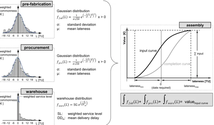
IV. ANALYSIS OF PROCEEDING SUPPLY PROCESSES Comparing the input curve of the Supply Diagram and the histogram of lateness distribution there are only two discrepancies to find: With histograms, the frequency of the lateness occurrences is measured, whereas with the Supply Diagram, the monetary value is. Moreover, the supply curve is cumulative while the histogram is not. These discrepancies can, however, be easily resolved by weighting the orders when creating the histogram with the individual values of the supply orders and summarizing these according to their lateness into classes.

pre-fabrication

Gaussian distribution

x > 0

σ: standard deviation

μ: mean lateness

L [TU] 18 12 6 -6 -12

-18 0

weighted commonness [€ ]

procurement

Gaussian distribution

x > 0

σ: standard deviation

μ: mean lateness

L [TU] 18 12 6 -6 -12

-18 0

weighted commonness [€ ]

warehouse

warehouse distribution

SL: weighted service level DDm: mean delivery delay weighted

commonness [€ ]

L [TU] 18 12 6 -6 -12

-18 0

weighted service level

∫

∫

∫

0 (date required)

lateness [TU]

latenessmin latenessmax

∑ input

completion curve

input curve

Va

lu

e

[€

]

assembly

Figure 5: Correlation between weighted output lateness of the supply process and the input curve of the Supply Diagram

Generating a Supply Diagram requires evaluating a large amount of feedback data, in particular the input dates and the dates of the completion of all components on the assembly stations. Since this is very laborious and data from the enterprises is frequently not available, it seems practical to pursue an approximate determination of a Supply Diagram with the help of common parameters.

Numerous experiences with practical data have shown that the lateness distribution of fabrication processes as well as procurement processes can be approximated by a Gaussian distribution. That is why the influence of the supply processes fabrication and procurement on the curve progression of the input curve of the Supply Diagram can be modeled by the Gaussian distribution function.

The schedule reliability and its lateness distribution of a warehouse differ from the other processes. A Warehouse rarely provides material too early. Lateness’s occur in case of shortages of material for example because of insufficient warehouse management. Other reasons for lateness could be caused by transportation problems. The service level of a warehouse is normally much better than a direct delivery from fabrication or procurement and the mean delivery delay is usually much lower. Besides the Gaussian function (Ffab(L) and Fpro(L)) fig. 5 shows a function (fware(L)) as a

first approach to approximate the lateness distribution of a warehouse with the help of a function including common key performance indicators.

After integrating each of the distribution function and summarizing them a function is formed to approximate the input curve of the Supply Diagram. One main benefit of this function is the consideration of KPI of the supply processes and the combination of them to one function because the influence of each single KPI on the input curve becomes

obvious. The correlation between the distribution of the lateness of the supply processes and the Supply Diagram opens up new possibilities for monitoring the supply situation of converging material flows. This cognition opens up the possibility of identifying cause and effect correlations between the supply processes and the supply situation while at the same time clearly facilitating and accelerating the determination of potential. With a Supply Diagram and the weighted distributions of output lateness of the supply processes it can be directly concluded how strong the individual supply processes influence the behavior of the Supply Diagram as well as which supply processes prevent the strived for synchronicity or cause disrupted WIP. With the help of the easy identification of the originator of a delayed supply it is much easier to develop measures to optimize an in due time supply of assembly processes.

Research is currently being conducted at the Institute of Production Systems and Logistics with regards to approximate the progression of the completion curve in order to achieve an as precise as possible approximation of the entire Supply Diagram. Factors that impact the completion curve such as the order structure and the arrival simultaneity of the components are being identified and their influence determined.

V.CONTRIBUTION TO A THEORY OF LOGISTICS A theory generally helps

to improve the comprehension of a system,

to systemize and to distribute developed knowledge and

to support decision processes with the help of the cognition of cause-effect interdependencies [7].

models which helps to plan and control an entire value chain is the long-term goal of the Institute of Production Systems and Logistics (IFA).

To realize this goal of a consistent and model-based representation of the value chain, it is necessary on the one hand to develop further models showing interdependencies between logistic objectives. On the other hand it is necessary to establish the correlation and the connection between several models. Fig. 6 shows a part of a value chain with the three different supply processes and a following assembly process. Also shown is a selection of existing models which are attached to the process types they can be applied to. The annotations of the axis indicate the several logistic objectives or KPI which are addressed by the models. Objectives (or related objectives) that are also used in the function to approximate the input curve of the Supply Diagram (see fig 5) are highlighted in fig. 6. Besides the mentioned above correlation to lateness distribution histograms at least one model per supply process has a connection to the function because of the same examined objectives: the Storage Operating curves depict the correlation between the service level and the delivery delay with the WIP. The Scheduling Adherence Operating Curve describes the relationship between schedule adherence and WIP. The schedule adherence is a key figure which can easily be calculated with a lateness distribution and is much related to the key figure lateness.

The links between the further models of the supply processes and the Supply Diagram will help to derive measures to improve the supply of a junction point in the material flow. Correlations between logistic objectives

which are decisive to evaluate improvement measures can be considered easily.

The investigation of the correlation between models of supply processes and the Supply Diagram will make a contribution to realize a comprehensive model of a value chain.

REFERENCES

[1] M. Schmidt, „Modellierung logistischer Prozesse der Montage,“ PZH Produktionstechnisches Zentrum GmbH, Garbsen, 2011.

[2] P. Nyhuis, R. Nickel, T. Busse, „Logistisches Controlling der Materialverfügbarkeit mit Bereitstellungsdiagrammen,“ ZWF, vol. 101, no. 5, pp. 265-268, 2006.

[3] H. Kettner, „ Neue Wege der Bestandsanalyse im Fertigungsbereich. Fachbericht des Arbeitsausschusses Fertigungswirtschaft (AFW) der Deutschen Gesellschaft für Betriebswirtschaft (DGfB).“ TU Hannover, 1976.

[4] P. Nyhuis, H. Rottbauer, „Erfolgsfaktoren und Hebel der Beschaffung im Rahmen eines Integrated Supply Managements,“ in Integrated Supply Management, R. Bogaschewsky (Ed.), Deutscher Wirtschaftsdienst, München, 2003, pp. 117-137.

[5] P. Nyhuis, H.-P. Wiendahl,. „Fundamentals of Production Logistics Theory, Tools and Applications,” Springer-Verlag, 2009.

[6] J. Steger, „Kosten- und Leistungsrechnung,“ 4th. ed., Oldenbourg, München, 2006.

[7] P. Nyhuis, “Entwicklungsschritte zu Theorien der Logistik,” in

Beiträge zu einer Theorie der Logistik, P. Nyhuis (Ed.), Springer-Verlag, 2008, pp. 1-16.

Author Information

Sebastian Beck is with Institute of Production Systems and Logistics, beck@ifa.uni-hannover.de

Matthias Schmidt is with Institute of Production Systems and Logistics, schmidt@ifa.uni-hannover.de

Peter Nyhuis is with Institute of Production Systems and Logistics, nyhuis@ifa.uni-hannover.de

Material flow warehouse

process time

wo

rk

Storage Operating Curve

WIP delivery delay service level

Storage Throughput Diagram

lateness value

3 3T 2T 0T

AVG2 1 1T 3T 1T

BVG1 4 2T 2T 0T

AVG3 2 2T 2T 0T

AVG2 5 1T 2T 0T

MVG1

time

wo

rk

/v

a

lu

e

Assembly Throughput Diagram

Network Theory Supply Diagram

material-buffer

supply processes _{staging of materials assembly}

assembly manufacturing

storage

procurement

time

wo

rk

Throughput Diagram

Schedule Adherence Operating Curce

WIP throughput

time output rate

WIP

sche

dule

adher

e

nce

Logistic Operating Curve

Lateness Distribution

lateness commonness

Schedule Adherence Operating Curce

Lateness Distribution

WIP

sched

ule

adher

e

nce

lateness commonness