Luiz Bevilacqua
[email protected] Instituto A. L. Coimbra/COPPE/UFRJ Programa de Engenharia Civil 21945-970 Rio de Janeiro, RJ, BrazilAugusto C. N. R. Galeão
[email protected] Laboratório Nacional de Computação CientíficaCoordenação de Mecânica Computacional 25651-075 Petrópolis, RJ, Brazil
Flavio P. Costa
[email protected] Universidade Estadual de Santa Cruz Departamento de Ciências Exatas e Tecnológicas BR-415, Ilhéus/Itabuna Ilhéus, BA, BrazilOn the Significance of Higher Order
Differential Terms in Diffusion
Processes
This paper deals with the analysis of diffusion coupled with temporary retention motivated by the challenge to solve the problem of population spreading. Retention may be associated to colonization of the occupied territory in this case. The discrete approach was selected to deal with this problem due to its relative simplicity and straightforward mathematical treatment. Two types of problems are analyzed namely: symmetric spreading with temporary retention, and propagation with temporary retention. It is clearly shown that higher order differential terms must be included in the governing equations of diffusion and propagation to represent the temporary retention effect. Specifically third and fourth order terms are associated to the retention effect in propagation and diffusion processes respectively. Control parameters regulating the relative influence of the diffusion and the retention terms in the governing equations come up naturally from the analysis. After the appropriated operations the finite difference equations reduce to partial differential equations. The control parameters are kept in the partial differential equations. These parameters are essential in the governing equations to avoid uncontrolled accumulation of particles due to the retention effect. The diffusion-retention problem appearing in several physicochemical problems are governed by the same equations derived here. The current literature refers to several types of diffusion-retention problems, but all solutions assume the classical second order equation as the basic reference. A short analysis of the equilibrium conditions for diffusion-retention problems with a source helps to show the coherence of the theory. In order to explore the potentialities of the discrete approach the problem of asymmetric distribution is also analyzed.
Keywords: discrete mathematics, diffusion, mathematical modeling, temporary retention
Introduction1
The advance of technological and scientific knowledge introduced new and sophisticated physicochemical processes to deal with new materials and new design concepts. Phenomena that were of little importance for the solution of the usual engineering problems cannot be disregarded anymore when dealing with modern engineering challenges.
Some phenomena that would be satisfactorily dealt with the continuum mechanics approach need now to be analyzed at nanoscales. This new trend fostered the search for the correspondence between the responses in terms of macro-variables and continuum mechanics on one hand and micro-variables and micro-mechanics on the other hand. Multiscale analysis, for instance, is a relatively new modeling methodology intended to make the bridge between the state variables at microscales and the corresponding ones at macroscales.
The new technological achievements require quick solutions to questions that are not yet completely understood. Pushed to solve a new problem, which is not seldom, the first approach is to apply the closest classical theory with some modification that hopefully would introduce the appropriate corrections. Experimental tests are then used to estimate the values of the critical parameters. This procedure may fail to provide a precise interpretation of the real phenomenon. The experimental results turn to be very restricted to specific problems and the results cannot be extrapolated to other similar cases.
The retention effect associated to particle diffusion is an example of such a case where the classical theory is not adequate. To the best of our knowledge, theories appearing in the current literature addressing this question assume the well-known second order parabolic equation as the basic governing equation of the
Paper accepted February, 2011. Technical Editor: Fernando A. Rochinha
dispersion process with retention. To solve the problem posed by the retention effect either some extra terms are added to the fundamental diffusion equation or the diffusion coefficient is expanded to introduce higher order terms. It is important to remark that when we talk about retention throughout this paper we are referring to temporary retention in contrast with permanent retention which may be simulated by the introduction of a sink in the governing equations.
This paper shows that a simple discrete approach may provide fundamental clues to define a consistent constitutive law adequate to take into account the retention effects in the diffusion process. Indeed, the finite difference equation modeling the retention-diffusion process, after taking the appropriate limits when the time interval and cell size tend to zero, is reduced to a linear fourth order partial differential equation provided that the problem is restricted to processes in thermodynamic equilibrium, the medium is homogeneous, the material coefficients are constant, and the dependent variable is smooth enough with respect to space and time. The new governing equation for the retention-diffusion problem may indeed be a fundamental reference for the determination of a general constitutive equation for the retention-diffusion phenomenon. For propagation processes the introduction of temporary retention requires a higher order term, a third order differential term as will be shown.
The presence of these new terms are associated with new physical constants that have a clear meaning and have to be evaluated with the help of experimental results. The theory developed here proposes a reliable model and therefore makes the experimental approach much more consistent. We have introduced also a classical example dealing with diffusion plus advection just to show how the discrete approach may be used to derive a large spectrum of evolution phenomena.
complementary fractions subjected to temporary retention. We concentrate our attention on the discrete approach motivated by the population dynamics problem. The detailed derivation of intermediate algebraic expressions is left to the appendix. The main text is restricted to the fundamental rules and the respective governing equations.
Nomenclature
B = source intensity k = mass fraction
K1 = mass transportation speed, wave speed
K2 = diffusion coefficient
K3 = retention coefficient for mass propagation
K4 = retention coefficient for diffusion processes
L0, L1 = length scale factors
pn = mass contents of the nth cell for the discrete approach
p = mass concentration for the continuum approach T0 = time scale factor
Greek Symbols
x = differential referring to the space variable
t = differential referring to the time variable
= wave length
ζ = wave amplitude
ω = frequency
ρR = ratio source intensity/retention coefficient for the diffusion
process
ρD = ratio source intensity/ diffusion coefficient
ρK = ratio retention coefficient for the diffusion process/ diffusion
coefficient
Symmetric Diffusion with Retention
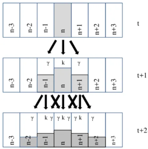
Consider the process depicted in Fig. 1. The rule governing the contents redistribution of each cell indicates that part of the contents denoted by kpn is retained in the nth cell and the exceeding part
denoted by
1k
pn 2 is evenly transferred to the neighboring cells at each time step. This means that the solution for this type of distribution varies slowly in time as compared with the solution of the classical diffusion problem. If k = 0 the problem is reduced to the classical Gaussian distribution. Translating this rule into algebraic expressions we get:
1 1 1
1 1
1
1
(1
)
1
2
2
t t t t
n n n n
p
kp
k p
k p
(1.a)
1
1 1
1
1
(1
)
1
2
2
t t t t
n n n n
p
kp
k p
k p
(1.b)Clearly, 0 ≤ k ≤ 1. The detailed algebraic operations are shown in the appendix B. It is important to notice that the equations must be worked out carefully, otherwise we could reach an equation that doesn’t reproduce the required solutions for the limits k = 1 and k = 0. Therefore, it is necessary to test the intermediate expressions at critical steps to make sure that the initial assumptions underlying equations (1.a,b) are preserved. This means that for k = 0 corresponding to no retention, the classical Gaussian distribution should be recovered and for the other limit when k = 1 the solution must be stationary, that is, the contents of each cell remain all the time constant.
n
n
n+1
n+1
n
+
2
n+2
n
+
3
n+3
n
-3
n
-3
n-2
n
-2
n
-1
n
-1 t
t+1
t+2
n n+1 n+2 n+3
n
-3 n-2 n-1
k
γ γ
kγ γkγ k γ
γ γ
Figure 1. Symmetric distribution with retention, γ = (1-k)/2.
The detailed derivation of all the intermediate steps leading to the expression (2) below is presented in the appendix B. Rewriting Eq. (B-6) deduced in the appendix B, we have:
3
4 2
4 2
4 2 2
1
2
2 2
t t t t
n k n n x
p k p p
t x x
t x x x
(2)
where 2pn
and 4pn stand for the second and fourth order
differentials. Let us take:
0 4 1
0 2 4 1 4
T
L
T
m
m
L
t
x
where L0, L1 and T0 are scale factors and xL0 mL1 m, and 2
0 m
T t
are the cell size and the time interval respectively. Substituting the above relations in Eq. (2) we get:
2 2
3 4 40 1
2 2 4
0 0
1
2
2
2
t t t t
n
k
nO
x
np
L
p
k
L
p
t
T
x
x
T
x
(3)
The scale factors L0 , L1 and T0 together with the parameter m provide very useful clues to define the sizes of space increment and time step for numerical integration of the finite difference equation.
Note that with k = 0,Eq. (3) reduces to the classical diffusion problem, that is no retention, and with k = 1,Eq. (3) represents a stationary behavior, for the right hand side term of (3) vanishes. Consequently, the time rate of the contents variation equals zero for all t for all the cells.
Calling 2 0
0 2 L 2T
K , 4 0
1 4 L 4T
K and assuming that p(x,t) is a sufficiently smooth function of x and t, we may take the limits as Δx→0 and Δt→0 to obtain:
0 2 0
0 2 2 0 2
T
L
T
m
m
L
t
x
1
2 22
1
4 44p p p
k K k k K
t x x
(4)
The fourth order term with negative sign introduces the effect of retention. The coefficients K2 and K4 are generalized constants. It is important to keep the parameters (1- k) and k(1-k) explicitly in the equation, because they are control parameters expressing the balance between diffusion and retention when both are activated simultaneously. For k close to zero, diffusion prevails and for k
close to one, retention prevails. The retention effect reaches its maximum for k = 0.5. Clearly, retention cannot be activated without diffusion, that is, while diffusion can take place without retention, the complementary process, that is, retention without diffusion is not possible. The generalization of the Eq. (4) to non-homogeneous media,where K2 and K4 are functions of x should keep the control parameters explicitly in the governing equation to take into account possible variations of the relative fractions of the diffusing particles and the temporarily trapped particles.That is, it is not advisable to incorporate (1-k) and k(1-k) in the coefficients K2 and K4.
According to the derivation above, the effect of temporary retention cannot be consistently modeled without the presence of the fourth order differential term. It is also remarkable that the discrete approach shows that non-linear terms are not required to represent temporary retention at least for the very simple case of homogeneous media and constant control parameters. This means, as it should be expected, that temporary retention belongs to the class of primary phenomena and, in general, is not a secondary perturbation on the diffusion process.
Asymmetric Diffusion without Retention
Now let us assume that the contents inside a given cell migrate to the neighboring cells according to a non-symmetric rule. We assume in this case that there is no retention. That is:
1 1
1 1
1
1 1
1 1
(1 ) 1 (5.a)
2 2
1 1
(1 ) 1 (5.b)
2 2
t t t
n n n
t t t
n n n
p k p k p
p k p k p
where –1 < k < 1. For k = 0 the problem reduces to the classical diffusion formulation. After carrying out careful algebraic operations, as shown in the appendix C, the following expression is obtained (C-4):
(6) 2
1
t -t 2
2 3
2 2 2 2 t
t
x x x p k x
x x x
p k x t t p
n
t t n
n
Let us take:
0 0
0 0
T L T
m m L t
x
0 2 1 0 2 1 2
T L T
m
m L t
x
where L0, L1 and T0 are scale factors and
x
L
0m
L
1m
, and tT0 m are the cell size and the time interval respectively.Introducing these expressions in Eq. (6) and taking the limit when 0
,
0
x t , we get:
x p k T L x
p k T L t p
0 0 2 2 2
0 2 1 1 2
Call 2 0
1 2 L 2T
K and
K
1
L
0T
0to obtain:
22
2
1
2 1p
p
p
K
k
K k
t
x
x
(7)The equation above reproduces the classical equation of diffusion with advection as it should be from the contents distribution rules introduced for the discrete approach. The finite difference formulation induces also here, as in the previous case, the preservation of the control parameter k explicitly in the governing equation. The parameter k controls the particle redistribution rate keeping the original meaning of the relative intensity of diffusion and propagation. For k1 propagation prevails to the right or to the left, and for
k
0
symmetric diffusion dominates. For the case presented here the flow velocity superposed to the diffusion process is equal to k, the unbalance factor in the redistribution process.Transport Phenomena with Retention
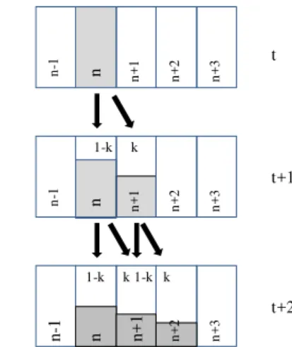
Consider now the distribution law that combines partial retention with contents transfer to a single cell located on the right or on the left. That is, the exceeding fraction of the contents of a given cell n, left after retention, is transferred either to the cell n+1or to the cell n−1. This means that the motion has a preferred direction as indicated by the arrows in the Fig. 2.
The analytical expressions of this law are easily written:
n
n
n+1
n
+
1
n
+
2
n
+
2
n
+
3
n
+
3
n-1
n
-1 t
t+1
t+2
n n+1 n+2 n+3
n
-1
1-k k
1-k k1-k k
Figure 2. Evolution of the contents profile for one-sided propagation with partial retention.
1
1
1 1
1
1 2 2
1
(1 ) (8.a)
(1 ) (8.b)
(1 )
t t t
n n n
t t t
n n n
t t t
n n n
p k p kp
p k p kp
p k p kp
(8.c)
In order to keep the correct response for the intermediate steps for all values of the parameter k, it is necessary to take double time step (t+1) and (t−1) for the calculation of the difference in time, that is, the calculations will be executed with the difference
1 t1
n t
n p
p . After a sequence of algebraic operations as shown in the appendix D we arrive at the following equation (D-5):
t tn
n t
n
x x
x x
p
x x
x x
p k k t t
t t
p
2 2
3 3
4
3 3 2
2 1
Again this expression satisfies the conditions required for k = 0 and k = 1. Now let us define:
0 0
0 0
T
L
T
m
m
L
t
x
0 3 1
0 3
3 1
1 3
T L T
m m
L t
x
where L0, L1 and T0 are scale factors,
3 1 1 0 m L m
L
x
and
m
T
t
0
are element size and time interval respectively. Substituting the above relations in the finite difference equation and taking the limits x0,t0 we get:
3 3
0 1
3
0 0
1 2
L L
p p p
k k k
t T x T x
Calling
K
1
L
0T
0and 33 1
2
0K
L
T
we finally get:
33 1 3 1
p p p
K k k K k
t x x
(9)
Clearly, Eq. (9) satisfies the phenomenological requirements imposed by the parameter k. For k = 0 the solution is stationary, and for k = 1 the solution falls in the category of a travelling wave. As in the previous problems, keeping the control parameters explicitly in the equation is helpful even for a continuum formulation.
It is remarkable the presence of the third order derivative in the equation of propagation with temporary retention. This term is required if temporary retention is to be taken into account. The derivation of a constitutive law for this kind of phenomenon starting from the generalized analysis of a continuum is a difficult task. The clue given by the discrete approach is fundamental to develop a consistent constitutive law.
Stability Analysis of the Diffusion-Retention Problem in the Presence of a Source
In this section the main focus is the stability condition of the solutions of the symmetric retention-diffusion problem coupled with an external source. Consider the problem of symmetric diffusion with retention. Let us assume that a certain amount t
n
g
is added to each cell after the contents redistribution is concluded at each
time step. With this simplified approach Eq. (B-5) in the appendix B may be rewritten to give:
1 2
3 1 41
2 4
t t t t t t
n n n n
p k p x k p g
(10)
Carrying out the necessary operations to transform Eq. (10) into a corresponding partial differential equation, as shown in the appendix, we have:
41 4 20 2
34 2 2
0 0
1 1
1
4 2
(11)
t t t t
n n n
t n
x
p L p L p
k k
t T x T x x
g t
Now if the filling rate is proportional to pn that is:
tn t
n
t g t Bp 0
lim
Expression (11) after taking the limit as Δx→0 and Δt→0 provided that the concentration p(x,t) is sufficiently smooth reads:
1
4 44
1
2 22p p p
k k K k K Bp
t x x
(12)
Equation (12) leads to a more complete modeling of population dynamics problems. The fourth order derivative was shown to be associated to a temporary retention of the cell contents and the source term Bp represents the added population proportional to the actual population. Therefore, Eq. (12) is a very good approximation to describe the expansion of living species. The coefficient B
represents the birth rate and K4 is proportional to the time needed for the offspring to mature till be ready to migrate. This approach is probably more realistic to represent population expansion than the classical second order diffusion equation.
The stability condition can be obtained from the time variation of the solution of Eq. (12) as a function of the relative values of the coefficients K2, K4 and B. Suppose a perturbation in the
neighborhood of an equilibrium state defined as:
exp(2 x )
p i t
(13)
Substituting this expression into Eq. (12) we have:
4
44 2 2
2
1 16 1
4
K k k K
k
B
If the solution given by (13) grows beyond any limit, it will be called unstable. Clearly, the sufficient condition for an unstable solution is ω > 0. Then:
1
16
1
04
4 4
4
2 2
2
k K k k K
B
which leads to the following condition for λ real and positive:
2 2
2
4 1
0 1 1 4
2 1
R D
D R
ρ ρ
π k
λ k ρ k ρ
where
4
K B R
and D B K2 represent respectively the
influence of the retention and diffusion coefficients in the generalized diffusion equation for a given value of the source B. Introducing the new parameter K K4 K2, Eq. (14.a) reads:
1 2
2
1 1 1
0 1 1 4
8 K 1 D K
k
k k
(14.b)
For a given wave length λ, the solution will grow without any limit if the condition (14) is satisfied. Or alternatively, for the solution to be stable the wave length must fall within the interval given by:
1 2
2
8 0
1 1 4
1
K
D K
kπ ρ
λ
k ρ ρ
k
(15)
1.0 0.5
0.0 1.00
0.75
0.50
0.25
0.00 k(1-k)
(1-k)
k
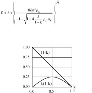
Figure 3. Variation of the characteristic control parameters for Eqs. (4) and (9).
Figure 3 shows the variations of the control parameters (1-k) and
k(1-k) as a function of k, the relative fraction of the temporarily trapped particles. For k close to 1, that is, high retention levels, the diffusion and retention multiplying parameters of the respective differential terms in the governing equation are small. For k close to zero, retention is small and diffusion prevails. In this case, the parameters multiplying the diffusion differential term in the governing equation are not affected by the retention effect and the parameters multiplying the retention differential term are small.
The stability conditions for the limiting cases of high retention activity k≈ (1-ε), on one hand, and of low retention activity k≈ ε, on the other hand, may be derived from Eq. (14.b). For the second case,
k≈ ε, the solution will be unstable if 1/ falls within the range given
by the inequality (16) below:
1 2
2
1 2
1 1 1
0 1 1 4
8 1
1
(16)
2 1
D K K
D
ε ρ ρ
λ π ε ρ ε
ρ
π ε
Since ε is small the stability range depends mainly on the ratio
D. Large values of
Dtend to destabilize the process, since the stability range decreases. In other words, large values of theexternal source and small values of the diffusion coefficient make the system unstable. Note that the stability of the solution may be considered as independent of the retention coefficient K4 in the presence of the other coefficients.
Now for processes with high retention activity we have k ≈ (1-ε).
The wave length range that keeps the solution unstable can be determined with the help of Eq. (14.b):
1 2
2
1 4 1
1 1 4
1 0
8 1
1 1
(17)
2 1
D K
K
D
K
ε ρ ρ ε
λ π ε ρ
ρ
π ε ε ρ
Since ε is small, 1/λ is very large and the instability range for the wave length is very big. Stability will be reached only for very short wave lengths. Now a process with high retention rate reduces the diffusion flow. This is reflected on the control parameter multiplying the diffusion coefficient in the governing equation. But low diffusion also reduces the retention activity as shown by the variation of the respective control parameter in Fig. 3. Therefore the perturbation introduced by the retention of a high fraction of particles in the system turns the process highly unstable independently of the values of
R,
Dor
K. The particles coming from the continuous feeding by the source tends to accumulate creating a positive feedback process, since the source intensity is proportional to the concentration level.The maximum value of the control parameter multiplying the retention differential term in the governing equation is reached for
k = 1/2. The system will be unstable if:
122
1 1 1
0 1 1 4
4 K D K
(18)
For small values of
Kthe inequality (18) may be reduced to the approximate relation:
1 1
0 2
2 D
(19.a)
A similar analysis for the case of diffusion without retention leads to
D
1 1
0
2
(19.b)
Conclusion
The theory developed above has introduced new results for diffusion and propagation. Although population dynamics was the motivation to solve the diffusion-retention problem, the most important problems are related to technological applications in engineering, biology chemistry and physics. Some of the problems belonging to these fields can be found in Atsumi (2002), D’Angelo et al. (2003), Brandani et al. (2000), Eon et al. (1997), Huang et al. (1982), Kirkland et al. (1990), Liu et al. (2002), Mota et al. (2004), Muhammed (2004), Nicholson et al. (1998). All the authors try to model the retention effect through some proper expansion of the diffusion coefficient or by adding some correction term in the equation. But since a general theory that couples diffusion and retention was missing each particular problem requires a different treatment.
This paper shows that a consistent theory including the phenomenon of temporary retention can be carried on with the help of a relatively simple discrete approach. The first argument that supports this statement is the straightforward derivation of the governing equation without any artificial manipulation or inappropriate theoretical corrections or additions. A second argument is the coherence with the expected results and the reduction of the diffusion coefficient intensity due to the retention effect. It is important to separate the meaning of the parameter k seen as a measure of the trapped particles and the role of k in the parameters (1−k) and k(1−k) controlling the phenomenological effectiveness of diffusion and retention respectively. For large fractions of trapped particles k≈1−ε the control parameter
multiplying the diffusion term is very small, reducing the diffusion current. This conclusion can also be found in the literature, but what is peculiar for our approach is that the diffusion is reduced due to a parallel phenomenon originated by the interactions particle-supporting medium whose effect is controlled by (1−k), leaving the material properties of the diffusion coefficient K2 unchanged. We don’t modify the actual material properties, retention is something in itself. The temporary retention effect in diffusion like processes, and propagation processes as well, introduces new differential terms in the classical equations.
As far as retention is concerned, the derivation of the governing equations shows very clearly how the term
4 44
1 kK p x
k , for
the symmetric diffusion case corresponding to the retention effect, comes into play. The multiplying parameter k(1−k) serves as control parameter weighing the influence of the retention term. This parameter avoids unrestrained growth of retention, that is, retention is only possible if diffusion is activated.
The present analysis holds for k constant assuming any value in the interval [0,1] depending on the physics of the problem. The retention effect reaches a maximum for k = 0.5. For the general case, however, it is plausible to assume k = k(p), which makes the solution more complex. In this case, the medium may have a saturation limit for the temporary retention activity given by a particular level of concentration, say p*, such that for k = k(p*) retention ceases. The present derivation, however, doesn’t apply for this more general hypothesis.
The equations obtained here serve as references for the investigation of more complex phenomena, where the coefficients
K1, K2, K3 and K4 are space and time dependent as well as the relative fraction k of trapped particle.
The relative roles of the terms in Eq. (12) on the growth process and on the stability conditions are also particularly important for modeling and simulation of social phenomena (Cavalli-Sforzza et al., 1993; Bettencourt et al., 2004; Gabay, 2007). Diffusion with
retention incorporating the contribution of some external source, representing the addition of new ideas, may model satisfactorily the knowledge dynamics in a production chain (Bevilacqua et al., 2005).
We would like to recall that the fourth order term has been used to model several physical and biological phenomena (Barabási et al., 1995; Myers et al., 1998; Mullins, 1957; Rubinstein et al., 1989; Schwartz et al., 2004). But to the best of our knowledge there is no reference of fourth order differential terms representing the temporary retention effect in the governing equations of an expanding population. It is possible to introduce fourth order terms by expanding Fick’s law (Cohen et al., 1981), but this approach requires the presence of non-linear terms in the differential equation, which is not necessary in the present theory, and furthermore doesn’t allow for the straightforward interpretation clearly shown here.
When a new theory is proposed the question of validation always comes into play. Certainly, the theory needs to be tested against appropriated experimental results. But it is equally important to have in hands a plausible theoretical development such that the experiments can be better planned. We believe that the present paper may serve as a guideline to new experiments. The material constants have to be determined to fit the corresponding coefficients in the equations developed here. Since the present approach introduces retention coefficient as an independent parameter characterizing explicitly the retention effect, it is expected that it represents a generalized interaction coefficient. That is, this new material constant should apply for a rather large spectrum of similar phenomena where diffusing particles interacts with the supporting medium, independently of the ongoing underlying phenomenon at microscales.
The mass transport in the positive x-direction leads also to very interesting result. Indeed the third order differential term makes the governing equation very similar to the famous Korteveg-deVries equation. Although the sign of this term entering the equation introduced here is negative, it is possible that the scattering effects are similar.
A final word now about the importance of multidisciplinary interaction among scientists and engineers coming from different knowledge background. Here a problem motivated by population dynamics could develop into a very rich conjecture about a set of very important questions raised by the developing technologies. Certainly, the problem of symmetric diffusion with retention under continuous feeding supplied by an external source as given by Eq. (12) represents much better the real evolution of living species on a substratum, considering reproduction and the maturation period of the infant population. But the relatively simple solution of the expanding population raised much more complex questions dealing with physicochemical phenomena. Nevertheless, the most fundamental concepts suggested by the population dynamics must be sustained in developing a more elaborated theory. This is another example that multidisciplinary collaboration usually converges for surprisingly good achievements.
Acknowledgements
We would like to thank Conselho Nacional de Pesquisas e Inovação (CNPq) for the partial support to this research through the Research Grant program, and Project: 480865/2009 -4; “Análise do efeito de retenção em problemas de difusão”.
References
Bettencourt, L.M.A., Cintrón-Arias, A., Kaiser, D.I., Castillo-Chávez, C., 2006, “The power of a good idea: Quantitative modeling of the spread of ideas from epidemiological models”, Physica A, Vol. 364, pp. 513-536.
Bevilacqua, L., Galeão, A., Bulnes, E., 2005, “Uma Análise Qualitativa da
Alguns Fatores Críticos na Dinâmica de uma Cadeia de Conhecimento”, Parcerias
Estratégicas –CGEE – Seminários Temáticos para a 3ª Conferência Nacional de Ciência, Tecnologia e Inovação, Vol. 20, Part 5, June, pp. 1395-1417.
Brandani, S., Jama, M., Ruthven, D., 2000, “Diffusion, self-diffusion and counter-diffusion of benzene and p-xylene in silicalite”, Microporous and Mesoporous Materials, Vol. 35-36, pp. 283-300.
Cavalli-Sforzza, L. et al., 1993, “Evolution of Social Groups”, Research Report, Santa Fe Institute.
Cohen, D.S., Murray, J.M., 1981, “A Generalized Model for Growth and Dispersal in A Population”, Journal of Mathematical Biology, Vol. 12, pp. 237-249.
Gabay M, “The effects of nonlinear interactions and network structure in
small group opinion dynamics”, Physica A, 378, (2007), 118-126.
Huang, J-C., Madey, R., 1982, “Effect of Liquid-Phase Diffusion Resistance on Retention Time in Gas-Liquid Chromatography”, Analytical Chemistry, 54-2, pp. 326-328.
Kirkland J.J., Boone L.S., Yau W.W., 1990, “Retention effects in thermal field-flow fractionation”, Journal of Chromatography A, Vol. 517, pp. 377-393.
Liu, H., Thompson, K.E., 2002, “Numerical modeling of reactive
polymer flow in porous media”, Computers and Chemical Engineering, Vol. 26, pp. 1595-1610.
Mota, M., Teixeira, J.A, Keating, J.B., Yelshin, A., 2004, “Changes in diffusion through the brain extracellular space”, Biotechnol. Appl. Biochem., Vol. 39, pp. 223-232.
Muhammad, N., 2004, “Hydraulic, Diffusion, and Retention Characteristics of Inorganic Chemicals in Bentonite”, PhD dissertation, Department of Civil and Environmental Engineering, College of Engineering, University of South Florida, June.
Mullins, W.W., 1957, “Theory of Thermal Grooving”, Journal of Applied Physics, 28-3, pp. 333-339.
Myers, T.G., 1998, “Thin films with high surface tension”, SIAM Review, 40-3, pp. 441-462.
Nicholson, C. and Sykova, E., 1998, “Extracellular space structure revealed by diffusion analysis”, Trends Neurosci, 21, pp. 207-215.
Rubinstein, J., Sternberg, P., Keller, J., 1989, “Fast reaction, Slow Diffusion, and Curve Shortening”, SIAM Journal of Applied Mathematics, 49-1, pp. 116-133.
Schwartz, L.W., Roy, V., 2004, “Theoretical and numerical results for spin coating of viscous liquids”, Physics of Fluids, 16-3, pp. 569-584.
Appendix
A. Definitions and elementary relations of finite difference mathematics
A.1. Definitons
Let f(x) be a function mapping the set of real numbers onto
itself, that is f:RR. All mapping considered in this paper is an isomorphism, that is, a one to one correspondence between points on the domain D(x) and on the image I(f(x)).
The following notation will be used throughout this paper:
kk
k
f
x
f
x
f
The mth order difference of f(x) centered at a point xk is written as m
k
f
. The mth order difference is the finite difference approximation of the mth derivative, m
mf x x
, of f(x).
We denote by O(Δx)
j algebraic expressions multiplied by terms
of order (Δx)j or higher*. For instance:
4 3 3
x b x a
x
, a
and b finite.
A function f(x) is said to belong to the class Cj –
j C x f( ) –
where j is either zero or an integer, if f(x) and all the derivatives
rr
x x
f
, r = 1,2… j, are continuous. By definition
x x f
xf
0 0
.
A.2. Some important relations to be used in the finite difference approach
1. The difference of order m > 1 is given by:
imi
i m i i z k k m
C
f
f
0
1
where
2 2 mod
m m z
and
!! !i i m
m Ci
m
The function {wmod2} returns the remainder of w divided by 2. The above expression for m
k
f
holds if f x
Cm, that is, that f(x)is continuous and all the derivatives up the order m as well. We also denote f(x) as sufficiently smooth to indicate that condition.
Examples:
1
f
kf
kf
k1 1
2
2
f
kf
kf
kf
k1 1
2 3
3
3
fk fk fk fk fk
2. The Taylor expansion for sufficiently smooth functions is:
2
1 1
2
(A-1)
k
k k k k
k k
k
f x
f f x f x x f x x x
x f
f x x
x
Similarly we have:
2 12 1 (A-2)
k
k k
f
f f x x
x
Now, for sufficiently smooth f(x) a similar expansion for the derivatives holds:
2
2 1
2 (A-3)
k k k
f f f
x x
x x x
Subtracting (A-1) from (A-2) and with (A-3) we have:
*
2 1
2 1 1
2
2 2
1 2 (A-4)
k k
k k k k
k
k k
f f
f f f f x x
x x
f
f f x x
x
Now, since the function f(x) is sufficiently smooth, the second derivative is finite and we may write:
21
2
f
x
f
k
k
Therefore, the differences centered at two neighboring points differ by terms of order (Δx)2. In general we have:
12 1 m
m m
k k
f f x
3. Another simple relation that will be helpful for the analysis is easily obtained with the help of the expressions deduced above:
2 2 1 1
2
2 1
2
1(A-5)
k k k k k k
k k k
f
f
f
f
f
f
f
f
f
x
B. Symmetric distribution with retention
The fundamental rule of contents redistribution reads:
1 1 1
1 1 1 1 1 (B-1a) (B-1b)
1
1
(1
)
1
2
2
1
1
(1
)
1
2
2
t t t t
n n n n
t t t t
n n n n
p
kp
k p
k p
p
kp
k p
k p
Reduction of the right hand side of equation (B-1b) to time t-1 leads successively to:
1
2 1 1 2 1 1 2 1 1 2 1 1 2 1 1 2 1 1 2 1 1 2 1 1 2 1 1 1 1 1 2 1 1 1 1 1 1 1 1 t n t n t n t n t n t n t n t n t n t n p k p k kp k p k p k kp k p k p k kp k p
1
4 1 ) 1 ( 1 2 1 1 1 2 2 1 1 1 1 1 2 1 t n t n t n t n t n t n t n t n p p p p k p p k k p k p Subtracting t n
p given by (B-1a) we get successively:
1
2
4 1 1 2 1 ) 1 ( 1 1 2 1 1 2 2 1 1 1 1 1 1 1 1 1 1 t n t n t n t n t n t n t n t n t n t n p p p k p p k p p k k p k k p p
1 1 1 1 1 1
1 1 1 1
1 1 1
2 2 1 1 2 1 1 2 4
t t t t t t t
n n n n n n n
t t t
n n n
p p k p p k p p p
k p p p
1 1 1 1 1 1
2 1 1 2
1 1 1 1 1
2 1 1 2
1
1 2 2 2
4 1
1 4 6 4 (B-2)
4
t t t t t t t
n n n n n n n
t t t t t
n n n n n
p p k p p p p p
k k p p p p p
1 1 1 1 1 1 1
2 1 1 2
1 1 1 1 1
2 1 1 2
1
1 2 2
4 1
1 4 6 4 (B-3)
4
t t t t t t t t
n n n n n n n n
t t t t t
n n n n n
p p k p p p p p p
k k p p p p p
Note that the left hand side of Eq. (B-3) represents the difference in time for the same cell n. In general, the time associated to the term t+k corresponds to t+k∆t, where ∆t is the time increment. All terms on the right hand side are referred to the same time t-1 and involve sum and difference operations of cell’s contents belonging to the interval n-2, n+2.
The term tn t
n p
p1
on the left hand side is the first order difference with respect to the variable t. We denote this difference, as explained in the appendix A, with the notation:
t n t n t
n p p
p
1
There are two terms on the right hand side of Eq. (B-3) of the
form 1 1 1 1 1 2 t K t K t
K u u
u
and one term of the form 1 2 1 1 1 1 1 1
2 4 6 4
t K t K t K t K t
K u u u u
u
. These expressions are the second and fourth order differences respectively with respect to the space variable, centered at the cell K. As introduced in appendix A we denote those differences with the notations:
k t K k t K k t K t k t
K u u u
u
1 1
2 2 k t K k t K k t K k t K k t K t k t
K u u u u u
u
4 2 1 1 2
4 6 4
Equation (B-3) can now be written in terms of the first, second and fourth order differentials:
2 2 41 1
1 1
1 (B-4)
4 4
t t t t t t t
n n n n
p k p p k p
With the result (A-4) from the appendix A, the above expression reduces to:
1
1 2
3 1 4 (B-5)2 4
t t t t t
n n n
p k p x k p
Clearly, Eq. (B-5) satisfies the physical requirements imposed by the limits of k, namely, k = 0 classical diffusion and k = 1 stationary solution. Rewriting (B-5) in terms of the appropriate ratios we get:
4 4 4 3 2 2 2 2 1 1 4 1 (B-6) 2 t n n t t n p pt k x k
t x x p x x x
C. Asymmetric distribution with no retention
Let us examine the case of asymmetric distribution without the retention term. This case is introduced just for the sake of testing the method. For this case it is expected the presence of a transportation term. It is diffusion with advection. The basic redistribution rule reads:
1 1 1 1 1 1 1 1 1(1 ) 1 (C-1a)
2 2
1 1
(1 ) 1 (C-1b)
2 2
t t t
n n n
t t t
n n n
p k p k p
p k p k p
Now, reducing the right hand side of equation (C-1b) to the time t-1 we get:
2 2
1 1 2 1 t-1
2 2
1
1
2 1
1
(C-2)
4
t t t
n n n n
p
k
p
k
p
k
p
Proceeding as before – appendix B – to find the difference in the contents of a general cell n, following the rules (C-1a) and (C-1b) corresponding to the time step {t+1,t} we get successively:
2 2
1 1 2 1 t-1
2 2
2
1 1 1 1 1
1 1 2 2
1 1 1 1
2 2 1 1
1 1 1 1 1
2 2 1 1
1
1 2 1 1
-4
1 1
- (1 ) 1 2
2 2 4
2 2 2 2
4 1
2 2 2
4
t t t t
n n n n n
t t t t t
n n n n n
t t t t
n n n n
t t t t t
n n n n n
p p k p k p k p
k
k p k p p p p
k
p p p p
p p p p p
(C-3)
Now, it is always convenient to test if the results obtained at each step reproduce the expected behavior according to (C-1a) and (C-1b). For this case, if k = 0 the solution should represent the classical diffusion equation, and for k = 1 the solution should reproduce a propagation towards the right and for k = –1 a propagation towards the left side. The following expressions confirm the expected behavior.
For k = 0 the previous equation reduces to:
1
31 1 1 2 1 1 2 1 2 2 1 2 2 4 1 x p p p p p p p p p p p t n n n t n n n n n n t n t n
Taking the limit of the finite difference expression above, the classical diffusion equation is obtained as expected. For k = 1 we get:
1 1 1
1 2
t t t t
n n n n
p p p p
Noting that the left hand side of this equation represents variation with respect to time and the right hand side variation with
respect to space; we may say that the above expression stands for the equation of propagation. Recalling the relations deduced in the appendix A further manipulation of equation (C-3) leads to:
1
1 1 1 1 2 2 1 2 2 1 2 1 1 1 1 1 2 2 1 2 1 1 1 1 1 1 1 2 2 1 1 2 1 2 1 1 4 1 2 2 1 4 1 2 2 1 4 1 t n t n t n t n t n t n t n t n t n t n t n t n t n t n t n t n p k p k p k p k p p p p k p p p p p p k p p
1
1 1 2 2 1 1 1 2 2 1 2 1 1 1 1 1 2 2 3 1 2 2 1 2 2 4 1 2 2 2 2 4 1 1 2 1 t n t n t n t n t n t n t n t n t n t n t n kp p k k kp p k k p p p p k x p k p p
1
1 1 2 1 2 1 1 1 1 1 2 1 2 1 1 3 1 2 2 1 2 2 2 2 2 1 1 2 1 t n t n t n t n t n t n t n t n t n t n t n p p p p p p k p p k k x p k p p
Now, introducing the notation defined above and rearranging the terms we get:
1
1 1 2 1 2 1 1 3 1 2 2 1 1 2 1 1 2 1 t n t n t n t n t n t n p p k p p k k x p k p
n
n
t tt
n k p x k p x
p
2 2 3 2
1 2 1
Or after introducing the appropriate ratios in the above expression with respect to x, t, we get:
3 2 t 2 2 2 2 t- t 2 1 2 (C-4) t t n n n k x p p t xt x x
x p x k x x
D. One-dimensional propagation with retention
The rule to be followed for this particular case reads:
1
1
1 1
1
1 2 2
1
(1 ) (D-1a) (1 ) (D-1b)
(1 )
t t t
n n n
t t t
n n n
t t t
n n n
p k p kp
p k p kp
p k p kp
(D-1c)