Comparison between Empirical Correlation and Computational Fluid Dynamics Simulation for the Pressure Gradient of Multiphase Flow

(1)

Comparison between Empirical Correlation

and Computational Fluid Dynamics Simulation

for the Pressure Gradient of Multiphase Flow

Yvonne S. H. Chang, T. Ganesan and K. K. Lau

Abstract - The objective of this research is to compare the use of empirical correlation with Computational Fluid Dynamics (CFD) simulation in determining the pressure gradient in two-phase flow pipelines at the same inlet condition. In this work, the empirical model of Beggs and Brill model had been used whereas the turbulent model applied in the CFD simulation was the Renormalization Group (RNG) k-ε model. A statistical analysis was conducted to determine the deviation in the values obtained by the CFD simulation as compared to those from the empirical correlation. It was found that the CFD results were in a good agreement with the findings obtained from the empirical correlation with a deviation of less than ±5%.

Index Terms - empirical correlation, Computational Fluid Dynamics, pressure gradients, two-phase flow

I. INTRODUCTION

Multiphase flow is defined as a flow with two or more distinct phases, which in this case is a liquid-gas flow. The prediction of its characteristics has not been easy since each segment of the flow map has significantly different energy requirements to sustain the flow and a real-life flow will jump from one segment to the next at an unpredictable time. In general, empirical correlations are used to deduce the pressure gradients in a multiphase flow pipeline [1]. For a single-phase flow, the pressure gradient equation is developed by using the conservation principles of mass and momentum. The same principles are used to calculate the pressure gradients for a multiphase flow. However the presence of an additional phase makes the development much more complicated.

Yvonne S. H. Chang, T. Ganesan and K. K. Lau are currently with Universiti Teknologi PETRONAS, Chemical Engineering Department, Bandar Seri Iskandar, 31750 Tronoh, Perak, Malaysia (phone: +60-5-3687644; fax: +60-5-3656176; e-mail: [email protected]).

The Beggs and Brill model [2] has been selected as the empirical correlation used in this work because it shows several significant features that set it apart from the other multiphase flow models. In this model, the slip condition and the flow pattern are considered in computing the pressure gradients along the pipelines. Depending on the established flow pattern, the liquid holdup and friction factor correlations can also be determined. Moreover, it is important to recognize that this model can deal with angles other than vertical upward flow. Consequently, it can be applied for hilly terrain pipelines and injection wells which are always encountered in the petroleum engineering. In short, the ‘Beggs and Brill’ model is considered classic in the field of multiphase flow and has been cited by several papers to be reliable for calculations involving large liquid mass input fractions and small diameter pipes at various orientation angles [2].

In the CFD simulation, both the boundary and operating conditions were determined. Then, the partial differential equations (PDE) or the Renormalization Group (RNG) k-ε model was selected. With the specified boundary conditions, the pressure profile was approximated numerically and thus solving the PDE. The convergence criterion and residuals were adjusted accordingly to obtain the best possible results. This was done with the aid of the CFD commercial software.

(2)

II. BEGGS AND BRILL MODEL

The Beggs and Brill model has been identified to be applicable in this research as it exhibits several characteristics that set it apart from the other multiphase flow models:

a) Slippage between phases is taken into account

Due to the two different densities and viscosities involved in the flow, the lighter phase tends to travel faster than the heavier one – termed as slippage. This leads to larger liquid hold-up in practice than would be predicted by treating the mixture as a homogeneous one.

b) Flow pattern consideration

Depending on the velocity and composition of the mixture, the flow behaviour changes considerably, so that different flow patterns emerge. These are categorized as follows:-segregated, intermittent and distributed. Depending upon the flow pattern established, the hold-up and friction factor correlations are determined.

c) Flow angle consideration

This model deals with flows at angles other than those in the vertical upwards direction.

Some assumptions had been used in the development of this correlation:

1. The two species involved do not react with one another, thus the composition of the mixture remains constant.

2. The gaseous phase does not dissolve into the liquid one, and evaporation of the liquid into gas does not occur.

The Beggs and Brill model [2] has the following pressure-gradient equation for an inclined pipe:

(1) (1)

Where dP/dL is the pressure gradient, f is the friction factor, ρn is the overall gas and liquid density relative to

their mass fraction, vm is the mean velocity, g is the

gravitational acceleration and Ek is a dimensionless

term.

III. CFD SIMULATION OF MULTIPHASE FLOWS

A. Renormalization Group

k

j e k j i i S Y G G x k x ku x k

t ⎟+ + − − +

⎟ ⎠ ⎞ ⎜ ⎜ ⎝ ⎛ ∂ ∂ ∂ ∂ = ∂ ∂ + ∂

∂ _ρ _ρ _α _μ _ρε

(2)

(3)

where the ρ is the fluid density, k is the kinetic energy, ε is the dissipation rate,

u

is the mean velocity, μ_e is the effective viscosity, α_k is the inverse effective Prandlt number for the k term, α_ε is the inverse effective Prandlt number for the

ε

term,

k G is

the generation of turbulent kinetic energy due to mean velocity gradients, G_b is the generation of turbulent kinetic energy due to buoyancy, Y_m is the contributions of the fluctuating dilation in compressible turbulence to the overall dissipation rate, S_k is the user defined source terms and C1e (1.42) and C2e (1.68) are the

empirical constants [6]

B. Volume of Fluid (VOF) Model

The Volume of Fluid (VOF) model [7] is used for the simulation of fluid characteristics in which there are more than one phases of fluids present in the flow. The phases of the fluids must not be mixing, i.e. not interpenetrating with each other. For every additional phase of the fluid, a supplementary variable is

K s m n E g d v f dL dP − + = 1 sin 2 2 θ ρ ρ

( )

(

)

(

G C G

)

C _k

k C x x u x

t j e k b e

e j i i 2 2 3

1 ρε

ε ε μ α ρε

ρε _ε ₊ ₊ _ε ₋ ∗

(3)

introduced in the volume fraction of the phase in the cell through the finite volume method.

The VOF model is suitable to be applied in cases under steady state condition. The properties of fluid obtained from the phases are in the form of volume averaged. However, these properties are subject to the volume fractions at specific locations.

The volume fraction of q_th fluid is denoted asα_q. In the VOF model, the following conditions apply: If

0

=

q

α , then there is no q_th fluid in the cell. If α_q=1, then the cell is full of q_th fluid. If 0<α_q<1, the cell contains a mix of q_th fluid with other fluids. Hence, by taking the

α

_q as a basis, the properties of fluid can be determined in the control volume through the finite volume method. On the other hand, the face fluxes for all the cells, including the fluxes at the interface, can be obtained through:

(

)

∑

=

+ Δ

− ₊ ₊

+

f

n f q n f n

q n q

U V

t 0

1 , 1 1

α α

α ₍₄₎

where Δt is the time-step and n+1 f

U is the fluid property at n+1.

IV. RESULTS AND DISCUSSION

A. Assumptions Used

In order to produce a valid comparison between both of the methods used, i.e. empirical correlation and CFD simulation, a few assumptions had been made. The assumptions made are as follows:

1. The flow is at steady state.

2. The flow is adiabatic, i.e. no heat transfer throughout the flow

3. The flow is isothermal, i.e. no temperature change during flow.

4. The flow is stratified and segregated, i.e. both the liquid and gas phases do not mix with each other 5. The pipe used is a commercial steel or wrought iron, with grade N80 and a relative roughness of 0.000045.

6. The inlet velocity or flow rate of liquid and gas is assumed to be the same.

7. There is no chemical reaction taking place throughout the flow.

8. There is no diffusion or phase generation throughout the flow.

9. Both the liquid and gas phases are flowing with a fully developed turbulent flow

The fluid properties used in this research are as follows [8]:

Operating Pressure, P = 7584280 Pa Operating Temperature = 104.44 oC

Density of oil @ 104.44oC, ρL = 704.4 kg/m3

Density of gas @ 104.44o_C,_ρ

G = 0.9849 kg/m3

Viscosity of oil @ 104.44oC, L = 0.000542 Ns/m2

Viscosity of gas @ 104.44oC, G = 0.0000143 Ns/m2

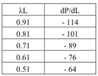
B. Pressure Gradients from Empirical Correlation

The pressure gradients at various mass fractions of liquid are as tabulated in Table 1.

Table 1: Pressure gradients at various mass fraction of liquid from empirical correlation

C. Pressure Gradients from CFD Simulation

A summary of the pressure gradients obtained for each mass fraction along with the corresponding residuals is as tabulated in Table 2.

Table 2: Pressure gradients and normalization of residuals at various mass fraction of liquid from CFD

simulation

Liquid Mass Fraction (kgliquid/kg

mixture)

Pressure Gradient (Pa/m)

Linear Estimate:

Norm of Residuals 0.91 - 118 557.5947 0.81 - 103 651.0205 0.71 - 93 967.7813 0.61 - 79 951.4034 0.51 - 62 1202.2071

L dP/dL

0.91 - 114

0.81 - 101

0.71 - 89

0.61 - 76

(4)

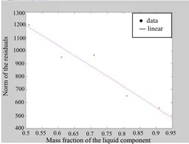
The linear estimate, which is represented in the form of normalization of residuals, is used to provide a conservative approximation of the pressure gradients obtained by CFD simulation (Table 2). Figure 1 shows the relationship between the normalization of residuals and the mass fraction of liquid obtained through CFD simulation.

Figure 1:Relationship between the normalization of residuals and the mass fraction of liquid

From Figure 1, as the mass fraction of liquid increases (which means the mass fraction of gas reduces), normalization of the residuals reduces, and vice versa. When the mass fraction of gas increases, the turbulence level in the flow increases because gases are generally more turbulent than their liquid counterparts at the same velocity. Consequently, non-linear or irregular pressure gradients were generated, and thus a greater deviation from the linear estimate, in cases with lower mass fraction of liquid.

D. Comparison between the empirical correlation and CFD simulation

The magnitude of deviation for the pressure gradients obtained from both the empirical correlation and CFD simulation was calculated by an error analysis equation as given below:

% 100

× − =

E E CFD P

P P P

D (5)

where D_P is the percentage of deviation, P_CFD is the pressure gradient obtained by CFD simulation andP_E

is the pressure gradient obtained by the empirical correlation. The results are as shown in Table 3.

Table 3:The pressure gradient and the linear estimate, norm of residuals that are

obtained from the Fluent software and the Matlab 7.1 software for a

variation of liquid mass fraction.

From Table 3, it is clear that the Dp of the pressure

gradients obtained by the CFD simulation relative to those obtained by the empirical correlation are quite small, i.e. less than 5%. The negative magnitudes obtained for PCFD and PE denote that the pressure

dropped progressively across the test section. However, with more boundary conditions that is more data on the nature of the flow a more reliable and accurate result can be obtained. This is because according to the Von Neumann criteria the stability of the flow is dependent on the bounded solution. If the solution is bounded then the flow is stable, and hence to obtain a bounded solution, sufficient data regarding the system or the flow is required. In CFD, the finite element method is utilized to solve the PDE numerically. Thus computational power is required to obtain a solution. Computational power plays a vital role in increasing the accuracy and the reliability of the data, which directly means that the higher number of iterations performed, the higher the accuracy.

V. CONCLUSION

The deviation of pressure gradients obtained through CFD simulation with respect to the Beggs and Brill empirical correlations was found to be relatively small, i.e. less than ±5%. Therefore, it can be concluded that the CFD simulation, which is more efficient and economic, can be used as an alternative to the empirical correlations to obtain the pressure gradients in two-phase flow pipelines. However, it is recommended that this research is repeated by comparing the CFD results with the data from experimental work. This will provide a more accurate analysis for multiphase pipeline designs and constructions.

Liquid Mass Fraction (kgliquid/kg

mixture)

CFD

P (Pa/m)

E P

(Pa/m)

P D (%)

0.91 - 118 - 114 3.5

0.81 - 103 - 101 2.0

0.71 - 93 - 89 4.5

0.61 - 79 - 76 3.9

0.51 - 62 - 64 3.1

N

o

rm

o

f th

e re

sid

u

als

1300 1200

1100 1000

900

800

700

600

500

400

0.5 0.55 0.6 0.65 0.7 0.75 0.8 0.85 0.9 0.95

(5)

ACKNOWLEDGEMENT

We wish to record our sincere gratitude to Universiti Teknologi PETRONAS (UTP). Apart from financial support, they made available to us research facilities and resources which were integral to this work. Thanks are also extended to A. P. Dr. Thanabalan Murugesen, who reviewed sections of the manuscript.

SYMBOLS

P pressure (Pa)

L pipe length (m)

d pipe diameter (m)

f friction factor

ρL liquid density (kg/m3)

ρG gas density (kg/m3)

ρn density of gas-liquid (kg/m3) L liquid mass fraction G gas mass fraction

L liquid dynamic viscosity (N s/m2) G gas dynamic viscosity (N s/m2)

n dynamic viscosity of gas-liquid (N s/m2) m mean velocity (m/s)

Fr Fraud number

HL(Ө) liquid holdup

REFERENCES

[1] Brill, J. P. and Mukherjee, H. (1999). Multiphase flow in wells. Monograph Volume 17, SPE, Henry L.Doherty Series.

[2] Beggs, H. D., and Brill, J. P., (1973). A study of two-phase flow in inclined pipes. Trans. AIME, 255, p. 607

[3] Ferziger, J. H. and Peric, M. (2002). Computational methods for fluid dynamics. Springer.

[4] Choudhury, D. (1993). Introduction to the renormalization group method and turbulence modeling. Fluent Inc. Technical memorandum TM-107.

[5] Biswas, G. and Eswaran, V. (2002). Turbulent flows: Fundamentals, experiments and modeling, Alpha Science International Ltd.

[6] Fluent Inc. (2001). Fluent 6 User’s Guide. India: Fluent Documentation Software.

[7] Manninen, M., Taivassalo, V. and Kallio, S. (1996). On the mixture model for multiphase flow. VTT Publications 288, Technical Research Centre of Finland.