Stability Analysis of BLDC Motor Drive
based on Input Shaping
M.Murugan#1, R.Jeyabharath*2 and P.Veena*2 ∗
Assistant Professor, Department of Electrical & Electronics Engineering, K.S.Rangasamy College of Technology,Tiruchengode, TamilNadu, India ; email: {[email protected]} #
Professor, Department of Electrical & Electronics Engineering, K.S.R. Institute for Engineering & Technology,Tiruchengode, TamilNadu, India
Abstract: The main objective of this work is to analyze the brushless DC (BLDC) motor drive system with input shaping using classical control theory. In this paper, different values of damping ratio are used to understand the generalized drive performance. The transient response of the BLDC motor drive system is analyzed using time response analysis. The dynamic behaviour and steady state performance of the BLDC motor drive system is judged and compared by its steady state error to various standard test signals. The relative stability of this drive system is determined by Bode Plot. These analysis spotlights that it is possible to obtain a finite-time setting response without oscillation in BLDC motor drive by applying input in four steps of different amplitude to the drive system. These analyses are helpful to design a precise speed control system and current control system for BLDC motor drive with fast response. The Matlab/Simulink software is used to perform the simulation.
Keywords: BLDC Motor, Input Shaping, Precise Speed Control
Nomenclature: r
qs
V
: q-axis equivalent stator voltage in voltsr qs
i
: q-axis equivalent stator current in ampss
L
: Equivalent stator self-inductance in henrys
R
: Equivalent stator winding resistance in ohmsP : Number of poles of motor
L
T
: Load torque of motor in N-mm
B
: Motor viscous friction coefficient in N-m/rad/secm
J
: Rotor inertia of motor in Kg-m2r
ω
: Angular speed of rotor in mechanical rad/ sece
T
: Electromechanical Torque in N-mA : Amplitude of Step input
I. INTRODUCTION
DC drives are widely used in applications such as rolling mills, paper mills, hoists, machine tools, excavators, cranes etc. because of reliability, good speed regulation, and adjustable speed, braking and reversing. But DC drives suffer from disadvantages imposed by the commutator segments and brushes. Sparking at the brushes limits both the highest speed of operation and the design capacity of the motor. Since the late 1960s, it has been predicted that ac drives would replace dc drives, however, even today, variable speed applications are dominated by dc drives. The earliest description of a brushless DC motor was in 1962 when Wilson and Trickey developed a “DC Machine with State Commutation”. A synchronous motor with speed sensors and inverter together constitute a BLDC motor. Hence instead of mechanical commutation, solid-state commutation is employed in BLDC motor drives. Because of high efficiency, high power factor and power density, BLDC motors have been widely used in a variety of applications in industrial automation and consumer electric appliances.
fast transient responses. In addition, stability analysis of the proposed control was made. Chung-Feng and Chih-Hui Hsu [2] suggested that the speed overshoot in a permanent magnet synchronous motor can be completely eliminated using Input Shaping Technique. This method gives much better transient performance with faster settling time. In this paper both the current and speed control systems are analyzed using time-domain analysis. Stability analysis has not yet been performed for the proposed speed control system.
Therefore, in this paper both the speed and current controller of the BLDCM drive are analyzed using the feedback control system of the drive. Then the transient state and steady state behavior of the control system are analyzed using conventional control theory. Also, the steady state performance of the drive system is analyzed by calculating its steady state error to step, ramp and parabolic inputs. The stability of the BLDCM drive is determined using frequency domain analysis.
II. MATHEMATICAL MODEL OF BLDC MOTOR
The design of the speed controller is important from the point of view of imparting desired transient and stead-state characteristics to the speed controller BLDC motor drive system [7]. The Fig. 1 shows the closed loop system of BLDC motor with both speed and current controller. The Fig. 2 shows the current controller of the BLDC drive system.
Fig. 1. Speed and q-axis Stator Current controller in the Closed Loop of BLDCM
Fig. 2. q-axis Current Controller in the Closed Loop of BLDCM
Under the assumption that =0, the system becomes linear and resembles that of a separately- excited dc motor with constant excitation. The block diagram derivation and derivation of speed controller are identical to those for a dc or vector controlled induction- motor – drive speed controller design. The q-axis voltage equation with the d-axis current being zero is given by,
r qs
r r
qs s qs s
d i
V
R i
L
d t
=
+
(1)( )
(
) ( )
r r
qs s s qs
V
s
=
R
+
sL
i
s
(2)The electromechanical torque equation is given by,
(
)
2
r
e L m m
d
P
T
T
J
B
r
dt
ω
ω
−
=
+
(3)(
)
(
)
2
e L m m rP
T
−
T
=
sJ
+
B
ω
(4)The electromagnetic torque is given by,
3
.
2 2
r r
e ds qs
P
2
3
2 4
r r
r
m m r ds qs t qs
d
P
J
B
i
K i
dt
ω
ω
λ
+
=
=
(6)where, 2
3
2 4
t dsP
K
=
λ
(7)After feedback the closed loop transfer function of the q- axis stator current controller can be obtained as,
* 2
( )
160000
( )
160
160000
r qs i r i qs
i
Y s
R s
=
i
=
s
+
s
+
(8)The closed loop transfer function of the speed controller is given by,
* 4 3 2
( )
256000000
( )
176
162560
2560000
256000000
s r
s r
Y s
R s
s
s
s
s
ω
ω
=
=
+
+
+
+
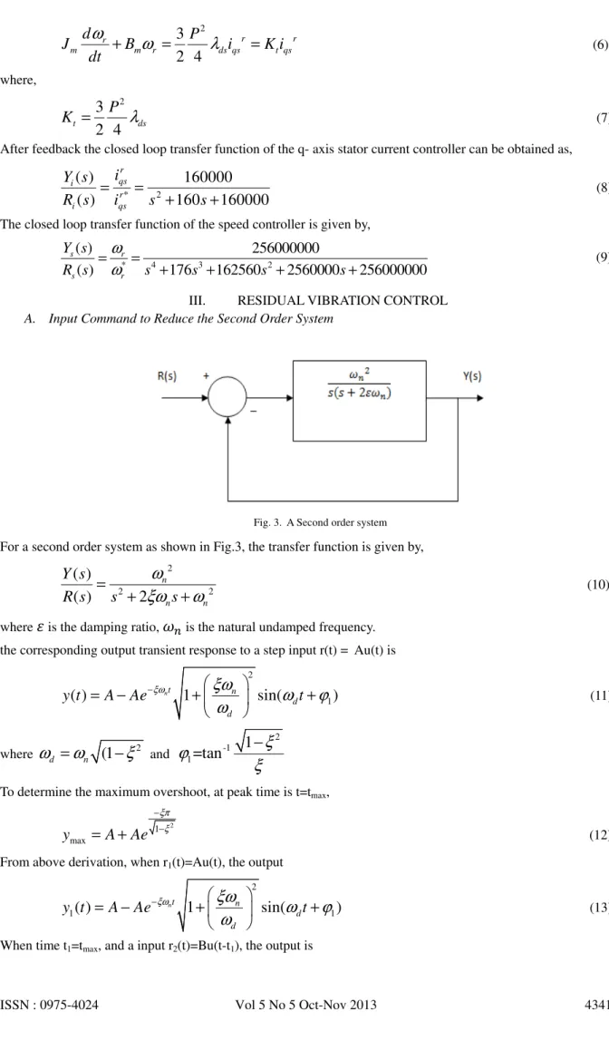
(9)III. RESIDUAL VIBRATION CONTROL A. Input Command to Reduce the Second Order System
Fig. 3. A Second order system For a second order system as shown in Fig.3, the transfer function is given by,
2
2 2
( )
( )
2
n
n n
Y s
R s
s
s
ω
ξω
ω
=
+
+
(10)where is the damping ratio, is the natural undamped frequency. the corresponding output transient response to a step input r(t) = Au(t) is
2
1
( )
nt1
nsin(
)
d d
y t
A
Ae
ξωξω
ω
t
ϕ
ω
−
=
−
+
+
(11)where
ω
d=
ω
n(1
−
ξ
2 and2 -1 1
1
=tan
ξ
ϕ
ξ
−
To determine the maximum overshoot, at peak time is t=tmax,
2 1 max
y
A
Ae
ξπ ξ
− −
=
+
(12)From above derivation, when r1(t)=Au(t), the output
2
1
( )
1
sin(
1)
nt n
d d
y t
A
Ae
ξωξω
ω
t
ϕ
ω
−
=
−
+
+
(13)1
2 ( )
2( ) 1 sin( 2)
n t t n
d d
y t B Be ξω ξω ω t ϕ
ω
− −
= − + +
14)
If H is the target, when t1=tmax,
Let A+B=H and the output y1(t)+y2(t)=H we get
1 1
2 2
( )
1 1 2
1
sin(
)
1
sin(
)
0
nt n n t t n
d d
d d
Ae
ξωξω
ω
t
ϕ
Be
ξωξω
ω
t
ϕ
ω
ω
−
+
+
+
− −+
+
=
(15)Let 2 1
E
e
ξπ ξ − −=
The amplitude of the first step is given by,1 H A E = + (16)
The amplitude of the second step is given by
B
=
AE
(17)1 2
1
nt
π
ω
ξ
=
−
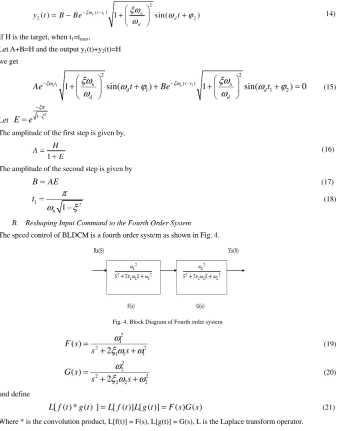
(18)B. Reshaping Input Command to the Fourth Order System
The speed control of BLDCM is a fourth order system as shown in Fig. 4.
Fig. 4. Block Diagram of Fourth order system
2 1
2 2
1 1 1
( )
2
F s
s
s
ω
ξ ω
ω
=
+
+
(19)2 2
2 2
2 2 2
( )
2
G s
s
s
ω
ξ ω
ω
=
+
+
(20)and define
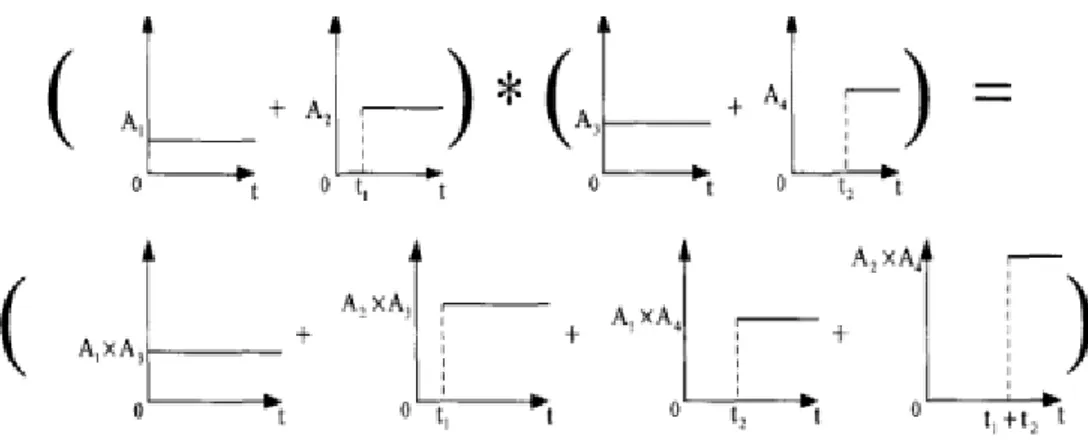
[ ( ) * ( ) ]
[ ( )] [ ( )]
( ) ( )
Fig. 5 Convolution Product Theorem for Fourth Order System
For residual vibration control, the two different inputs with different time for f(t) are A1 and A2. Then 1 1
1
1
A
E
=
+
(22)1 2 1
1
E
A
E
=
+
(23)1 2 1 1 1
E
e
ξ π ξ − −=
(24)1 2
1
1
1t
π
ω
ξ
=
−
(25)
For residual vibration control, the two different inputs with different time for g(t) are A3, and A4 respectively. Then, 3 2
1
1
A
E
=
+
(26)2 4 2
1
E
A
E
=
+
(27)2 2 2 1 2
E
e
ξ π ξ − −=
(28)2 2
2
1
2t
π
ω
ξ
=
−
(29)The amplitude of the four step input is given by,
1 3 2 3 1 4 2 4
(
A
*
A
) (
+
A
*
A
) (
+
A
*
A
) (
+
A
*
A
) 1
=
(30)IV. TRANSIENT RESPONSE ANALYSIS
Since the physical speed control system involves energy system, the output of the system, when subjected to an input, cannot follow the input immediately but exhibits a transient response before a steady state can be reached. The transient response of a practical speed control system often exhibits damped oscillations before reaching a steady state. So to analyze a control system, it is necessary to examine the transient response behaviour of the control system [4]. The transfer function of speed control system is given by,
2 2
( )
256000000
1
( )
(
161.5028021
158604.5849) (
14.49719789
1614.076919)
Y s
The system response can be analyzed to a step input as follows.
Let
.
then,2 2
0.418
256000000
1
( )
(
161.5028021 158604.5849) (
14.49719789
1614.076919)
Y s
s
s
s
s
s
=
×
×
+
+
+
+
(32)Taking Inverse Laplace Transform, we get,
80.84 80.84
7.23 7.23
( ) 0.418 0.009704
sin(389.88
78.29) 0.01
sin(389.88 )
0.43445
sin(39.53 - 79.63) 0.016029
sin(39.53 )
t t
t t
y t
e
t
e
t
e
t
e
t
− −
− −
=
−
−
−
+
−
(33)Fig. 6. Step response curve when u (t) =0.418
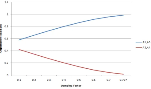
Fig. 6. shows the step response curve of the speed control system. From the analysis, it can be seen that, the first peak over shoot occurs at 0.08sec and the magnitude is given by 0.66. The first undershoot occurs at 0.16sec and the corresponding magnitude is 0.28. The second peak overshoot occurs at 0.24sec and the magnitude is obtained as 0.49. The second undershoot occurs at 0.32 sec and corresponding magnitude is obtained as 0.37. The transient response of the speed control system subjected to single step input exhibits damped oscillations and the response is settled at ts =0.77sec which is a larger one. Fig. 7. shows the variation of step inputs A1, A2, A3 and A4 with respect to damping factor.
Fig. 7.Variation of A1, A2, A3 and A4 with damping factor
correspondingly the values of A2 and A4 are 0.2. From the analysis, it can be seen that these values of A1, A2, A3 and A4 give an output response with zero residual oscillations. Similarly, we can find the values for input with respect to any other values of damping factor.
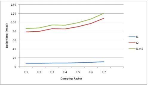
Fig. 8. Variation of delay times with damping factor
The Fig. 8 shows the variation of delay times t1, t2 and t1+t2 with respect to damping factor. It can be seen that the delay times increases with damping factor. From this analysis, it shows that the delay times corresponding to
0
.
4
gives an output response with zero oscillations. Thus, the precise speed control of BLDC motor can be achieved by properly choosing the damping factor and delay time of the step input. The Fig. 9 shows four step input given to the speed control system of the BLDCM drive system.Fig. 9. Four Step Input
For a damping factor
.
,.
;.
.
;.
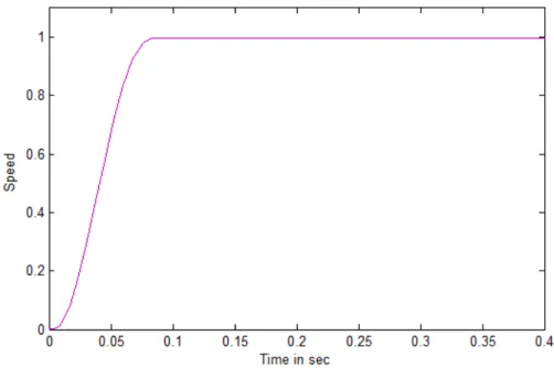
Fig. 10.Output Response after input shaping
Fig. 10. shows the speed response when four step input is given to the drive. The foregoing analysis shows that, the speed response is settled at ts=0.085sec without any damped oscillations. Thus it is concluded that, after input shaping the settling time is so much reduced from 0.77sec to 0.085 sec.
V. STABILITY ANALYSIS OF CONTROL SYSTEMS A. Steady State Error and Error Constants
The steady state performance of the speed controller system can be judged by its steady state error to Step, Ramp and Parabolic inputs. Based on block diagram one can calculate the steady state error ωe(s) due to unit step input1/s,unit ramp input 1/s2 and unit parabolic input 1/s3.[4] The steady state error and static error constants are obtained as, for unit step input Kp= ∞ and ωe(s) = 0; for unit ramp input Kv=100 and ωe(s) = 0.01and for unit parabolic input Ka=0 and ωe(s) = ∞. From the foregoing analysis, it is seen that the higher the static error coefficients, the smaller the steady state error. The type 4 speed control system can follow a step input with zero actuating error at steady state. This system can follow the ramp input with a finite error. This analysis also indicates that the speed control system is incapable of following a parabolic input.
B. Frequency Domain Analysis
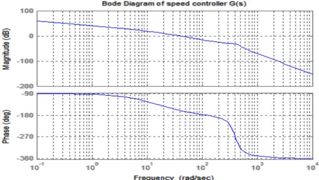
The frequency response of a control system presents a qualitative picture of the transient response. Such analysis of a control system indicates graphically what changes have to be made in the open-loop transfer function in order to obtain the desired transient response characteristics [5]. The Bode diagrams of both controllers are shown in Fig. 11 and Fig. 12.
Fig. 12. Bode Plot of Speed Controller
From the frequency response analysis, phase margin and gain margin for current controller is obtained as 200 and 47.0719dB and for speed controller 200 and 16.906dB.
VI. RESULTS AND DISCUSSION
In this paper both the speed controller and current controller of the BLDC motor drive are analyzed using the control system model of the drive system. The transient and steady state behaviour of the control system is analyzed using conventional control theory. The step response curve shown in Fig.4 shows that the first peak overshoot occurs at 0.08sec and the magnitude is given by 0.66. The first trough occurs at 0.16 sec and corresponding magnitude is 0.28. The response is settled with a settling time of 0.77sec which is a large one for any drive system. Therefore, instead of giving a single step reference input, multiple step input is given to the drive system. From Fig.6 it can be seen that the response is settled at ts=0.085sec without any oscillations. Thus it is concluded that after input shaping the settling time is so much reduced from 0.77sec to 0.085 seconds. From Fig.5 it can be seen that the magnitude of A1 and A3 increases with damping factor and the magnitude of A2 and A4 decreases with damping factor.
Also the steady state performance of the system is analyzed by calculating its steady state error for step, ramp and parabolic inputs. The steady state errors for step, ramp and parabolic inputs are obtained as 0, 0.01 and ∞. The static error constants are obtained as Kp=∞, Kv=100 and Ka=0. Thus we can conclude that the higher the static error coefficients, the smaller the steady state error. Also, the drive system can follow a step input with zero actuating error at steady state and is incapable of following a parabolic input. This system can follow the ramp input with a finite error.
The stability of both controllers are carried out which is shown in Fig.11 and Fig.12. From the Bode diagram, the phase margin and gain margin for current controller is obtained as 200 and 47.0719dB and for speed controller is obtained as 200 and 16.906dB. It shows that both gain margin and phase margin are positive for speed and current control systems. Therefore, both controllers are stable systems. This analysis will be helpful to design a stable control system for BLDC motor drives.
ACKNOWLEDGMENT
We would like to thank Dr.S.Ravi, Professor, Department of Electrical and Electronics Engineering, Nandha Engineering College, Erode for his technical guidance, and support of this work. The author would like to thank Prof. Palaniappan, Department of English, K.S.Rangasamy College of Technology, Tiruchengode for providing language help and proof reading of this work.
REFERENCES
[1] R. Venkitaraman, B.Ramaswami, “Thyristor Converter-Fed Synchronous Motor Drive”, Electric Machines and Electromechanics, 6: 433-449, 1981.
[2] Chung-Feng Jeffrey Kuo, Chih- Hui Hsu “Precise Speed Control of a Permanent Magnet Synchronous Motor”, International Journal of Advanced Manufacturing Technology. 28: 942-949, May 2005.
[3] Ching-Tsai Pan, Emily Fang, “A Phase-Locked-Loop-Assisted Internal Model Adjustable-Speed Controller for BLDC Motors”,IEEE Transactions on Industrial Electronics, Vol.55, No.9, pp 3415-3425, Sep 2008.
[4] Katsuhiko Ogata, Modern Control Engineering (International Edition) Prentice- Hall of India, New Delhi 1988 [5] I.J Nagrath and M.Gopal, Control Systems Engineering, New Age International (P) Limited, New Delhi, December 1981. [6] Vedam Subramanyam, Electric Drives, Tata McGraw- Hill Publishing Company Limited, New Delhi, 1994.
[7] R.Krishnan,” Electric Motor Drives, Modelling, Analysis and Control”, PHI Learning Private Limited, New Delhi, 2009.
[9] R.C.Becerra and M.Ehsani, “High Speed Torque Control of Brushless PM Motor” IEEE Transaction on Industrial Electronics, Vol.35, August 1988.
[10] Acarnley, P.P., Watson, J.F., “Review of position sensorless operation of brushless permanent-magnet machines” IEEE Transactions on Industrial Electronics., 53(2):352-362, 2006.
[11] Halvaei Niasar, A., Moghbelli, H., Vahedi, A., “A Novel Sensorless Control Method for Four-switch, Brushless DC Motor Drive without Using Any 30 Degree Phase Shifter”. Proceedings IEEE Int. Conference on Electrical Machines and Systems, p.408-413, 2007. [12] Su.G.J., McKeever, W., “Low-cost sensorless control of brushless DC motors with improved speed range” IEEE Transactions on Power
Electronics, 19(2):296-302, 2004.
[13] Texas Instruments, TMS320LFLC240xA DSP Controllers Reference Guide—System and Peripherals. No.SPRU357B, 2001. [14] Anand Sathyan, N.Milivojevic,y-J Lee and M.Krishnamoorthy, “An FPGA-Based Novel Digital PWM Control Scheme for BLDC
Motor Drives” IEEE Transaction on Industrial Electronics” Vol.35, pp 3040-3049 August 2009. Biography
M.Murugan was born in Tamil Nadu, India. He is graduated in 2002 from Madurai Kamarajar University, and post graduated in 2004 at Anna University, Chennai. He is a Research scholar in Anna University of Technology, Coimbatore. He is currently working as an Assistant professor in the department of EEE at K.S.Rangasamy College of Technology, Tiruchengode from June 2004 onwards. He is guiding UG, PG Students. He is an ISTE member. He published 5 international/national conferences. His research interest involves in Power Electronics and drives, Special Electrical Machines and Control Systems
Dr.R.Jeyabharath was born in Tamil Nadu, India. He is graduated in 2001 from Madurai Kamarajar University, and post graduated in 2003 at Bharathiar University, Coimbatore, and he got doctoral degree in 2008 at Anna University, Chennai. He is currently working as a Professor in the department of EEE at K.S.Rangasamy College of Technology, Tiruchengode from June 2003 onwards. He is guiding UG, PG Students. He is an ISTE, IETE member. He published 15 international/national conferences, journals. His research interest involves in Power Electronics and drives, Special Electrical Machines and optimization techniques.