DOI: 10.7508/ceij.2016.02.003
* Corresponding author E-mail: [email protected]
215
Assessment of Ilam Reservoir Eutrophication Response in Controlling
Water Inflow
Nourmohammadi Dehbalaei, F.1, Javan, M.2*,Eghbalzaeh, A.3, Eftekhari, M.4 and Fatemi, S.E.5
1
M.Sc., Department of Civil Engineering, Razi University, Kermanshah, Iran.
2
Assistant Professor, Department of Civil Engineering, Razi University, Kermanshah, Iran.
3
Assistant Professor, Department of Civil Engineering, Razi University, Kermanshah, Iran.
4
Director of Water Resource Institute (WRI), Tehran, Iran.
5
Assistant Professor, Department of Water Resources Engineering, Campus of Agriculture and Natural Resource, Razi University, Kermanshah, Iran.
Received: 02 Oct. 2015; Revised: 02 Aug. 2016; Accepted: 04 Oct. 2016
ABSTRACT: In this research, a 2D laterally averaged model of hydrodynamics and water quality, CE-QUAL-W2, was applied to simulate water quality parameters in the Ilam reservoir. The water quality of Ilam reservoir was obtained between mesotrophic and eutrophic based on the measured data including chlorophyll a, total phosphorus and subsurface oxygen saturation. The CE-QUAL-W2 model was calibrated and verified by using the data of the year 2009 and 2010, respectively. Nutrients, chlorophyll a and dissolved oxygen were the water quality constituents simulated by the CE-QUAL-W2 model. The comparison of the simulated water surface elevation with the measurement records indicated that the flow was fully balanced in the numerical model. There was a good agreement between the simulated and measured results of the hydrodynamics and water quality constituents in the calibration and verification periods. Some scenarios have been made base on decreasing in water quantity and nutrient inputs of reservoir inflows. The results have shown that the water quality improvements of the Ilam reservoir will not be achieved by reducing a portion of the reservoir inflow. The retention time of water in reservoir would be changed by decreasing of inflows and it made of the negative effects on the chlorophyll-a concentration by reduction of nutrient inputs and keeping constant of discharge inflow to reservoir, the concentration of total phosphorus would be significantly changed and also the concentration of chlorophyll-a was constant approximately. Thus, the effects of control in nutrient inputs are much more than control in discharge inflows in the Ilam reservoir.
216
INTRODUCTION
Eutrophication is the enrichment of an aquatic ecosystem with additional nutrients from different pollution sources such as point and nonpoint sources. Some quality problems likediurnal variations in dissolved oxygen concentration and pH, hypoxic condition and etc. in the bottom are caused by an overabundance ofalgae biomass. The mass transport formula including the advection and dispersion equations, exogenous environmentalfactors (e.g., water temperature, riverine nutrient loads) and interactive biochemical kinetics are effective factors on phytoplankton dynamics (Karamouz and karachian, 2011; Kuo et al., 2006; Liu et al., 2009). Various management techniques such as reducing external nutrient source, hypolimnetic aeration, hypolimnetic withdrawal, artificial circulation, nutrient diversion, dilution and etc. are selected to manage and maintain water quality in lakes and reservoirs (Kuo et al., 2006; Liu et al., 2009; Garrell et al., 1977; Irianto et al., 2012). To improve the eutrophication in the reservoir, much effort has been made to reduce the external loading of phosphorus. Some reservoirs rapidly respond to such reductions (Kuo et al., 2006; Liu et al., 2009) but a delay in reservoir recovery is often seen (Messer et al., 1983; Dodds, 1992; Dzialowski et al., 2007). Water quality models are one of the best available tools used to determine the quantitative relationship between pollutant loads and water quality responses in water bodies. In the last decade, the CE-QUAL-W2 model has been widely used for modeling reservoirs in around the world (Gelda et al., 1998; Chung and Oh, 2006; Kim and Kim, 2006; Fang et al., 2007; Ma et al., 2008; Chung and Lee, 2009; Lee et al., 2010; Dai et al., 2012; Amarala et al., 2013). Wu et al. (2004) simulated the eutrophication in the Shihmen reservoir by the CE-QUAL-W2
217 eutrophication management in the Mingder reservoir. They showed that load reduction will change the water quality in this reservoir. Etemad-Shahidi et al. (2009) applied the CE-QUAL-W2 model to determine total maximum daily load (TMDL) of total dissolved solids during a two years’ period in the Karkheh reservoir. Yu et al (2010) described the influence of a diffuse pollution on a natural organic matter (NOM) in the Daecheong reservoir by using the CE-QUAL-W2 model. Liu and Chen (2013) assessed the effect of the withdrawal level on stratification patterns and suspended solids concentration in the Shihmen reservoir by the CE-QUAL-W2 model. Deus et al. (2013) simulated the eutrophication in the Tucurui reservoir by this model and investigated various management scenarios to improve the eutrophication of the Tucurui reservoir. Park et al (2014) applied the CE-QUAL-W2 model to predict the pollutant load released from each reservoir in response to different flow scenarios. Zouabi-aloui et al. (2015) used the CE-QUAL-W2 model to simulate the impact of various water withdrawal scenarios in thermal stratification and water quality in the Sejnane reservoir.
The Ilam reservoir with a capacity of 71 million cubic meters is one of the two main sources of drinking water in Ilam city. The water taste and odor problems of the Ilam reservoir interested us to model the eutrophication in this reservoir. In this study, the laterally averaged two-dimensional CE-QUAL-W2 model was calibrated and verified by existing observation data in the Ilam reservoir. Then the calibrated model was used to evaluate the effect of using different management scenarios on chlorophyll a and total phosphorus concentrations.
STUDY AREA
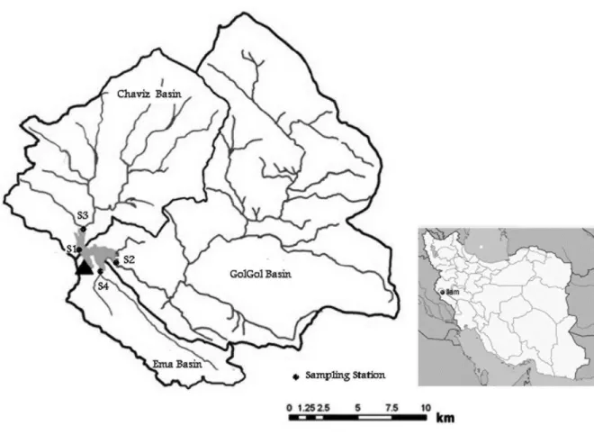
218
Fig. 1. Location of Ilam reservoir and the sampling point
Table 1. The trophic state of the reservoir in the various month at the dam station (S1)
Month TP
(mg/l) Trophic State
chlorophyll-a
(µg/l) Trophic State
Subsurface Oxygen Saturation (%)
Trophic State
July 943 Eutrophic 7.7 Mesotrophic 16 Mesotrophic
August 48 Eutrophic - - 14 Mesotrophic
September 195 Eutrophic 0.036 Oligotrophic 16 Mesotrophic
October 217 Eutrophic 1.17 Oligotrophic 16 Mesotrophic
November 100 Eutrophic 0.35 Oligotrophic 37 Mesotrophic
December 205 Eutrophic 0.4 Oligotrophic 59 Mesotrophic
April 72 Eutrophic 0.16 Oligotrophic 42 Mesotrophic
May 82 Eutrophic 0.36 Oligotrophic 52 Mesotrophic
June 118 Eutrophic 0.16 Oligotrophic 43 Mesotrophic
Model Description
In this study, the CE-QUAL-W2 model was selected to simulate the eutrophication process in the Ilam reservoir. This numerical model is a finite difference, laterally averaged, 2D hydrodynamics. It has been improved for the last three decades and also is supported by the US Army Corps of
219 nutrients, algal groups and organic matter can be simulated by the CE-QUAL-W2 model. Any combination of water quality parameters can be included or excluded from the numerical simulation. Due to assume lateral mixing, the CE-QUAL-W2 model is suited for relatively long and narrow water body that water quality gradient is in the longitudinal and vertical direction. In this model, the governing equations are the horizontal momentum equation, the continuity equation, the constituent–heat transport equation, the free water surface elevation equation, the hydrostatic-pressure equation and the state
equation (Cole and Wells, 2008).
Model Inputs
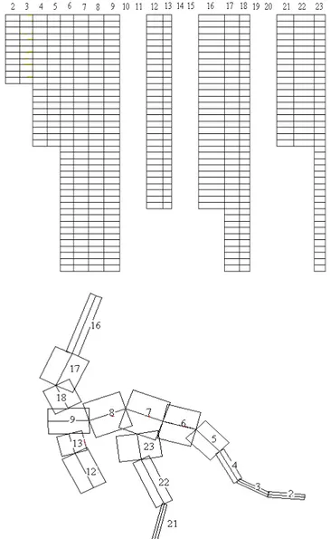
In the CE-QUAL-W2 model, the reservoir is divided into a number of segments linked together to form the system. Four branches water body of the Ilam reservoir was divided into sixteen segments with a length of 500 m to 700 m and layers with a depth of 1 m.Figure 2 shows the numerical model grids for the Ilam Reservoir. In addition to the Golgol, Chaviz and Ema rivers, a part of the reservoir water body located near the dam is also considered as a branch.
220 The CE-QUAL-W2 hydrodynamic model was calibrated using the year 2009 data and the year 2010 data were used for the numerical model validation. The modeling period was from July 27 2009 to June 14 2010 and the modeling start time was at
24:00 o’clock on January 1 2009. The
maximum time step and time step fraction were selected 1 hour and 0.8 in the simulation, respectively. The inputs of the numerical model were reservoir bathymetry, branches discharge, temperature and water quality, meteorological parameters and reservoir outflows. The grid dimensions were specified by three parameters: the length of each segment, the thickness of each layer and the width of the segment at each layer. The meteorological data generally are air temperature, dew point temperature, cloud coverage and wind speed and direction. The surface boundary conditions of the CE-QUAL-W2 model were constituted with these meteorological data. The requiredmeteorological data has been extracted from the Ilam synoptic stations. In this numerical simulation, the daily hydrology data and three-hourly
meteorology data were entered into the CE-QUAL-W2 model. Numerical simulations of the Ilam reservoir were divided into two main phases. The hydrodynamics and temperature at the first phase and then water quality constituents including ammonium, nitrate, phosphate, dissolve oxygen, silica and chlorophyll a have been simulated.
Hydrodynamics Results
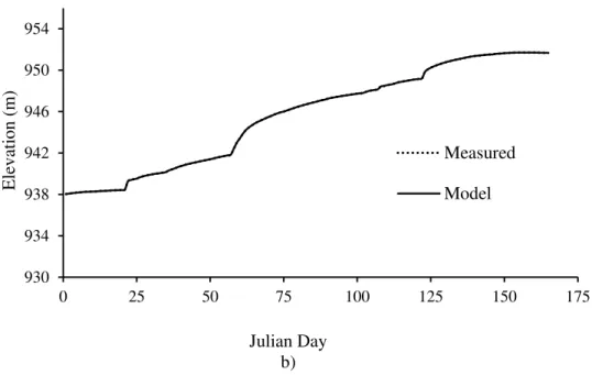
In the Ilam reservoir simulation, the calibration process was begun with the water balance. The water level was calibrated and verified using the daily data. Figure 3 shows the comparison of the simulated and measured water level. The mean absolute error (MAE) of the simulated water level was respectively 0.05 and 0.04 m for the year 2009 and 2010 therefore the flow balance was ensured in the model. The simulation and measurement results indicate that the water surface elevation gradually decreases and reaches the lowest level in the late autumn of 2009 and then gradually increases and reaches a peak level in the late spring of 2010.
930 932 934 936 938 940 942 944 946
0 50 100 150 200 250 300 350 400
Elev
ation
(m
)
Julian Day a)
Measured
221
Fig. 3. Comparison of the simulated and measured water surface elevation, a) the calibration period, b) the
verification period
The water temperature data was used to evaluate the hydrodynamics results of the numerical model. The temperature profiles were calibrated and verified using monthly data collected in 2009 (July to December) and 2010 (March to May), respectively. The light extinction coefficient is one of the key parameters in the modeling of the temperature distribution. Before simulating the reservoir temperature, this coefficient was determined from the measured Secchi Disk depth using the following relationship (Etemad-shahidi et al., 2009)
(1)
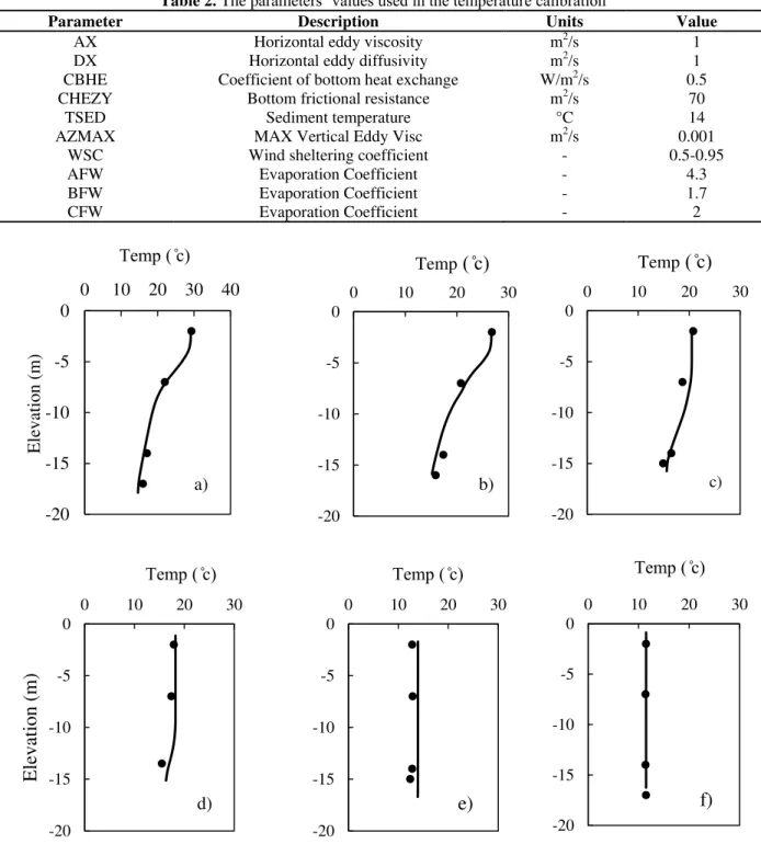
where λ and Zs: are light extinction coefficient (m-1) and depth of Secchi disk (m), respectively. After performing numerous runs of the model for calibrating the temperature distributions, the appropriate values of the coefficients such as horizontal eddy viscosity and diffusivity, sediment heat exchange coefficient, bottom frictional resistance, wind sheltering coefficient, maximum vertical eddy viscosity and
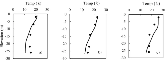
evaporation coefficients were determined and listed in Table 2. Figures 4 and 5 show the calibration and verification results for the temperature profile, respectively. As seen, the numerical model has successfully simulated the variations of the water column temperature in both stratified and well-mixed conditions. The MAE and maximum error of the simulated temperature were respectively 0.72 °C and 1.18 °C. Figure 6 shows that the simulated temperatures are within ±15% of the measured ones. In the Ilam reservoir, thermal stratification has started at the beginning of the spring (early April) and reached its maximum during the summer. The maximum temperature difference between the upper and lower layers is about 13 °C and the thermocline layer with a thickness of about 5 m is formed in the reservoir in the summer. The surface cooling and wind mixing induce the fall overturn of the water column in the late October. A complete vertical mixing has been observed in the late November and the reservoir has remained well-mixed during the winter (Figure 4).
930 934 938 942 946 950 954
0 25 50 75 100 125 150 175
Elev
ation
(m
)
Julian Day b)
Measured
222
Table 2. The parameters’ values used in the temperature calibration
Parameter Description Units Value
AX Horizontal eddy viscosity m2/s 1
DX Horizontal eddy diffusivity m2/s 1
CBHE Coefficient of bottom heat exchange W/m2/s 0.5
CHEZY Bottom frictional resistance m2/s 70
TSED Sediment temperature °C 14
AZMAX MAX Vertical Eddy Visc m2/s 0.001
WSC Wind sheltering coefficient - 0.5-0.95
AFW Evaporation Coefficient - 4.3
BFW Evaporation Coefficient - 1.7
CFW Evaporation Coefficient - 2
Fig. 4. Comparison of measured and simulated temperature profiles in the calibration period, a) Julian day = 208, b)
Julian day = 238, c) Julian day = 273, d) Julian day = 299, e) Julian day = 335 and f) Julian day = 364 -20
-15 -10 -5 0
0 10 20 30 40
Elev
ation
(m
)
Temp ( ̊c)
a)
-20 -15 -10 -5 0
0 10 20 30
Temp( ̊c)
b)
-20 -15 -10 -5 0
0 10 20 30
Temp( ̊c)
c)
-20 -15 -10 -5 0
0 10 20 30
Eleva
ti
on
(m
)
Temp ( ̊c)
d)
-20 -15 -10 -5 0
0 10 20 30
Temp ( ̊c)
e)
-20 -15 -10 -5 0
0 10 20 30
Temp ( ̊c)
223
Fig. 5. Comparison of measured and simulated temperature profiles in the verification period, a) Julian day = 105, b)
Julian day = 133 and c) Julian day = 165
Fig. 6. Comparison of the measured and simulated temperature data
Water Quality Results
For simulating the water quality of the Ilam reservoir, the dissolved oxygen, chlorophyll a and nutrient concentrations at the Golgol, Chaviz and Ema rivers confluence with the reservoir were entered as inlet boundary conditions. In Figures 7 and 8, the simulated water quality results including DO, phosphate, ammonium, silica, nitrate and chlorophyll a are compared with the measured data at the dam site in 2009. After numerous runs of the CE-QUAL-W2
model, the calibrated kinetic coefficients and constants for the water quality simulation were determined and listed in Table 3. In general, they are consistent with literature values (Afshar and Saadatpour, 2009, Cole and Wells, 2008). Several statistical methods including mean absolute error (MAE) and root-mean-square error (RMSE) were used to compare the simulated and measured results in the calibration and verification periods.
-30 -25 -20 -15 -10 -5 0
0 10 20 30
Elev
ation
(m
)
Temp ( ̊c)
a)
-30 -25 -20 -15 -10 -5 0
0 10 20 30
Temp ( ̊c)
b)
-30 -25 -20 -15 -10 -5 0
0 10 20 30
Temp ( ̊c)
c)
0 5 10 15 20 25 30 35 40 45
0 10 20 30 40
Te
m
pe
ra
tur
e
(S
im
ul
at
ed)
( ̊C
)
Temperature (Observed) ( ̊C)
- 15% Error Line + 15% Error Line
224 -20
-15 -10 -5 0
0 2 4 6 8 10 12
Ele
va
ti
on
(m
)
Do ( mg/l)
a)
-20 -15 -10 -5 0
0 2 4 6 8 10 12 Do (mg/l)
b) -20 -15 -10 -5 0
0 2 4 6 8 10 12 Do (mg/l)
c)
-20 -15 -10 -5 0
0 2 4 6 8 10 12
Ele
va
ti
on
(m
)
Do (mg/l)
d)
-20 -15 -10 -5 0
0 2 4 6 8 10 12 Do (mg/l)
e)
-20 -15 -10 -5 0
0 2 4 6 8 10 12 Do (mg/l)
f)
-20 -15 -10 -5 0
0 1 2 3
Ele
va
ti
on
(m
)
Phosphate (mg/l)
a)
-20 -15 -10 -5 0
0 1 2 3
Phosphate (mg/l)
b)
-20 -15 -10 -5 0
0 1 2 3
Phosphate ( mg/l)
225 -20
-15 -10 -5 0
0 1 2 3
Ele
va
ti
on
(m
)
Phosphate (mg/l)
d)
-20 -15 -10 -5 0
0 1 2 3
Phosphate (mg/l)
e)
-20 -15 -10 -5 0
0 1 2 3
Phosphate (mg/l)
f)
-20 -15 -10 -5 0
0 0.3 0.6 0.9
Ele
va
ti
on
(m
)
Ammonuim (mg/l)
a)
-20 -15 -10 -5 0
0 0.3 0.6 0.9 Ammonuim (mg/l)
b)
-20 -15 -10 -5 0
0 0.3 0.6 0.9 Ammonuim (mg/l)
c)
-20 -15 -10 -5 0
0 0.3 0.6 0.9
Ele
va
ti
on
(m
)
Ammonuim (mg/l)
d)
-20 -15 -10 -5 0
0 0.3 0.6 0.9 Ammonuim (mg/l)
e)
-20 -15 -10 -5 0
0 0.3 0.6 0.9 Ammonuim (mg/l)
f)
-20 -15 -10 -5 0
0 5 10 15 20
Ele
va
ti
on
(m
)
Nitrate ( mg/l)
(a)
-20 -15 -10 -5 0
0 5 10 15 20
Nitrate ( mg/l)
b)
-20 -15 -10 -5 0
0 5 10 15 20
Nitrate (mg/l)
226
Fig. 7. Comparison of the simulated and measured water quality profiles in the calibration period ((-) Modeled, (•)
Measured), a) Julian day = 208, b) Julian day = 238, c) Julian day = 273, d) Julian day = 299, e) Julian day = 335 and f) Julian day = 364
-20 -15 -10 -5 0
0 5 10 15 20
Ele
va
ti
on
(m
)
Nitrate (mg/l)
d)
-20 -15 -10 -5 0
0 5 10 15 20
Nitrate (mg/l)
e)
-20 -15 -10 -5 0
0 5 10 15 20
Nitrate (mg/l)
f)
-20 -15 -10 -5 0
0 2 4 6 8 10
Ele
va
ti
on
(m
)
Silica (mg/l)
a)
-20 -15 -10 -5 0
0 2 4 6 8 10
Silica (mg/l)
b)
-20 -15 -10 -5 0
0 2 4 6 8 10
Silica (mg/l)
c)
-20 -15 -10 -5 0
0 2 4 6 8 10
Ele
va
ti
on
(m
)
Silica (mg/l)
d)
-20 -15 -10 -5 0
0 2 4 6 8 10
Silica (mg/l)
e)
-20 -15 -10 -5 0
0 2 4 6 8 10
Silica (mg/l)
227
Fig. 8. Comparison of the simulated and measured chlorophyll a concentration in the calibration period, a) Top layer
b) Bottom layer
Table 3. Coefficients and constants used in the calibrated model of the water quality
Parameter Description Units Value
AG Algal grow rate (20 °C) day-1 0.66
AM Algal mortality rate for algal day-1 0.1
AS Algal settling rate day-1 0.1
AE Algal excretion rate for algal day-1 0.04
AR Algal dark respiration rate day-1 0.04
ASAT Algal light saturation W/m2 50
AHSP Algal half-saturation P g/m3 0.003
AHSN Algal half-saturation N g/m3 0.014
ASAT Saturation light intensity W/m2 50
NH4DK Ammonia decay rate day-1 0.001
NO3DK Nitrate decay rate day-1 0.03
PSIS Particulate silica settling velocity m/day 0.05
PSIDK Particulate silica decay 1/day 0.003
SOD Sediment oxygen demand g o2 m-2 day-1 0.7
0 2 4 6 8 10 12 14 16
0 100 200 300 400
Ch
lo
rop
hyll
a (
m
g/
l)
Julian day a)
Measured
Model
0 0.2 0.4 0.6 0.8 1
0 100 200 300 400
Ch
lo
rop
hyll
a (
m
g/
l)
Julian day b)
Measured
228
Calibration Period
Oxygen is an essential element for all organisms into aquatic ecosystems. According to Environment Protection Agency (EPA), larval life stages of many fish and shellfish species can be compromised when dissolved oxygen is less 5 mg/l for long periods. In a reservoir, the dissolved oxygen calibration is an important step for obtaining a useful model (Nielsen, 2005). The basic parameter influencing the modeling results of the dissolved oxygen is the sediment oxygen demand (SOD) (Chen et al., 2012). The parameter value of the sediment oxygen demand was determined so that a good agreement between the simulated and measured dissolved oxygen concentrations had been achieved. By the CE-QUAL-W2 model, the seasonal variations of the DO were well simulated in the reservoir and the simulated results were reasonably matched with the measured ones (Figure 7). At the surface layer of the Ilam reservoir, the DO concentration ranges are from 5.2 to 9 mg/L. During the summer and autumn seasons, the DO concentration is below the water quality criteria provided by EPA (Figure 7). The EPA water quality criteria states that phosphates concentration should not exceed 0.025 mg/l within a lake or reservoir. According to the measured data, the phosphate concentration of the Ilam reservoir is higher than drinking water standards during all months in which the measurements have been performed. Because of releasing phosphorus from the bottom sediments into water column under anoxic conditions, the available phosphorus has been increased within the reservoir water. The ammonium concentration is generally lower at the water surface due to algal uptake and higher at the bottom where the phytoplankton growth is dependent to the light limitation (Figure 7). The ammonium concentration is too higher than drinking water standards (0.5 mg/l) at the
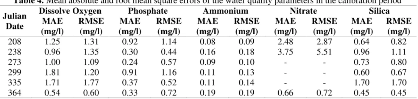
lower layers from August to December. After carbon, nitrogen is the second important component in the phytoplankton feeding processes. In this study, the nitrate decay rate was determined 0.03 day-1. A good agreement between the simulations and measurements of the ammonium and nitrate is observed (Figure 7 and Table 4). Silica is a limiting factor for diatoms and silica seasonal variations affect the diatoms growth. Diatoms are a major group of algae and second group of algae in the Ilam reservoir (Mahab Qods, 2010). The simulated and measured silica concentrations are compared with together in Figure 7 which indicates a good agreement between them. During the summer, when the stratification is evident, the simulations and measurements indicate that the silica concentration is higher at the bottom than the surface.
229
Table 4. Mean absolute and root mean square errors of the water quality parameters in the calibration period
Julian Date
Dissolve Oxygen Phosphate Ammonium Nitrate Silica
MAE (mg/l)
RMSE (mg/l)
MAE (mg/l)
RMSE (mg/l)
MAE (mg/l)
RMSE (mg/l)
MAE (mg/l)
RMSE (mg/l)
MAE (mg/l)
RMSE (mg/l)
208 1.25 1.31 0.92 1.14 0.08 0.09 2.48 2.87 0.64 0.82
238 0.96 1.35 0.30 0.44 0.16 0.18 3.75 5.51 0.96 1.11
273 1.00 1.09 0.24 0.57 0.09 0.10 - - 0.73 0.80
299 1.81 1.20 0.91 1.16 0.11 0.13 - - 0.60 0.67
335 1.71 1.77 0.37 0.52 0.11 0.14 - - 1.70 1.70
364 0.54 0.60 0.33 0.72 0.19 0.19 0.66 0.72 0.45 0.45
Verification Period
Model validation is possibly the most important step in the model building. There are many techniques including, comparison to other models, face validity, historical data validation, parameter variability – sensitivity analysis, predictive validation that can be utilized to verify a model. In this study, the historical data validation is selected for verifying the model. In this method, the parts of the data are used to build the model and the remaining data are used to test validity of the previously evaluated coefficients. For verification of the model, data from year 2010 were used. Verification results of the
numerical model are presented in Figure 9. Table 5 presents the verification results of MAE and RMSE between model results and observations. The means absolute errors are 1.21 mg/l, 0.19 mg/l, 2.85 mg/l, 0.1 mg/l, and 0.46 mg/l for DO, total phosphorus, nitrate, ammonium, and silica, respectively. The corresponding RMSE values are 1.43 mg/l, 0.21 mg/l, 4.31 mg/l, 0.12 mg/l and 0.57 mg/l, respectively. In Figure 9 and Table 5, a reasonable agreement between the model results and field measurements is observed. Therefore, this numerical model is appropriate for evaluation future management strategies.
Table 5. Mean absolute and root mean square errors of the water quality parameters in the verification period
Julian Date
Dissolve
Oxygen Total Phosphorus Ammonium Nitrate Silica
MAE (mg/l)
RMSE (mg/l)
MAE (mg/l)
RMSE (mg/l)
MAE (mg/l)
RMSE (mg/l)
MAE (mg/l)
RMSE (mg/l)
MAE (mg/l)
MAE (mg/l)
105 0.96 1.10 0.22 0.25 0.10 0.11 3.36 4.91 0.59 0.73
133 1.45 1.68 0.20 0.21 0.05 0.07 3.78 5.38 0.20 0.26
165 1.23 1.46 0.16 0.17 0.15 0.16 1.41 1.61 0.60 0.61
-30 -25 -20 -15 -10 -5 0
0 2 4 6 8 10 12
Ele
va
ti
on
(m
)
Do (mg/l)
(a)
-30 -25 -20 -15 -10 -5 0
0 2 4 6 8 10 12 Do (mg/l)
(b)
-30 -25 -20 -15 -10 -5 0
0 2 4 6 8 10 12 Do (mg/l)
230
Fig. 9. Comparison of the simulated and measured water quality profiles in the verification period ((-) Modeled, (•)
Measured), a) Julian day = 105, b) Julian day = 133 and c) Julian day = 165 -30 -25 -20 -15 -10 -5 0
0 1 2 3
Eleva ti on (m ) Phosphate (mg/l) (a) -30 -25 -20 -15 -10 -5 0
0 1 2 3
Phosphate (mg/l) (b) -30 -25 -20 -15 -10 -5 0
0 1 2 3
Phosphate (mg/l) (c) -30 -25 -20 -15 -10 -5 0
0 0.3 0.6 0.9
Ele va ti on (m ) Ammonuim (mg/l) (a) -30 -25 -20 -15 -10 -5 0
0 0.3 0.6 0.9 Ammonuim (mg/L) (b) -30 -25 -20 -15 -10 -5 0
0 0.3 0.6 0.9 Ammonuim (mg/l) (c) -30 -25 -20 -15 -10 -5 0
0 10 20 30
Ele va ti on (m ) Nitrate (mg/l) (a) -30 -25 -20 -15 -10 -5 0
0 10 20 30
Nitrate (mg/l) (b) -30 -25 -20 -15 -10 -5 0
0 10 20 30
Nitrate (mg/l) (c) -30 -25 -20 -15 -10 -5 0
0 2 4 6 8 10
Eleva ti on (m ) Silica (mg/l)
(a) -30
-25 -20 -15 -10 -5 0
0 2 4 6 8 10
Silica (mg/l) (b) -30 -25 -20 -15 -10 -5 0
0 2 4 6 8 10
Silica (mg/l)
231
MODEL APPLICATION
As mentioned earlier, the Ilam reservoir inflow is the discharge sum of Golgol, Chaviz and Ema rivers at the confluence with the reservoir. Based on the hydrological data, Golgol, Chaviz and Ema rivers respectively supply 68%, 23% and 9 % of the total annual inflow of the Ilam reservoir. The effects of various management scenarios on the chlorophyll a and total phosphorus concentrations were investigated. Simulations were executed for fifth scenarios: reference scenario (first scenario), the Ema river diversion (second scenario), the Ema and Chaviz rivers diversion (third scenario), total reduction of nutrient loads derived from the Ema river (fourth scenario) and total reduction of nutrient loads derived from Chaviz and Ema rivers (fifth scenario). The reference scenario corresponds to the actual situation and the results of the calibrated model used for this scenario. For the second and third scenarios, it was assumed that a diversion weir is constructed in the confluence of rivers with the reservoir and thus prevents the entering water from these rivers to the reservoir. Therefore, about 9% of the total annual inflow of the Ilam reservoir is diverted in the Ema river diversion (second scenario) and about 32% of the total annual inflow of the Ilam reservoir is diverted in the Chaviz and Ema rivers (third scenario). For the fourth and fifth scenarios, it was assumed that the best management approach in the watershed was applied to achieve nutrient load reduction from rivers. For this purpose, the concentration of nutrients including phosphate, ammonium, Silica and nitrate in rivers was reduced. All other reservoir condition was kept identical. Concentration duration curves of chlorophyll a and depth-averaged total phosphorus yielded by the numerical simulation of these scenarios are illustrated in Figures 10 and
11, respectively. The Ema river diversion (second scenario) reduces 3% depth-averaged total phosphorus concentration in 17% of the time and increases 44% chlorophyll a concentration in 44% of the time. The 9% reduction of the inflow to the Ilam reservoir (second scenario) leads to increase the water retention time which has a considerable effect on the chlorophyll a concentration. The inflow variations to the reservoir have little effect on the thermal stratification. The Ema and Chaviz rivers diversion (third scenario) decreases 23% depth-averaged total phosphorus concentration. The chlorophyll a concentration is increased 200 percent at the third scenario (32% reduction of the inflow). The water retention time affects the chlorophyll a concentration with inflow reduction (2nd and 3rd scenario). Hence, the chlorophyll a concentration within the reservoir approximately is independent of the nutrient loads input changes. On the other, it significantly affects the phosphors concentration of the reservoir. The total reduction of the nutrient loads entered by Chaviz and Ema rivers decreases 30% depth-averaged total phosphorus concentration in 17% of the time.
232
Fig. 10. Duration curves of chlorophyll a concentration at the top layer of the reservoir in the various scenarios
Fig. 11. Duration curves of total phosphorus depth-averaged concentration in the various scenarios
CONCLUSIONS
In this research, a 2D laterally averaged model of hydrodynamics and water quality, CE-QUAL-W2, was applied to simulate variations in the water quality parameters of the Ilam reservoir. The water quality of Ilam reservoir was obtained between mesotrophic and eutrophic based on the measured data including chlorophyll a, total phosphorus and subsurface oxygen saturation. The CE-QUAL-W2 model was calibrated using the year 2009 data and the year 2010 data were used for the numerical model validation. The
comparison of the water surface elevation with the measurements indicated that the flow was fully balanced in the numerical model.The numerical model has successfully simulated the variations of the water column temperature in both stratified and well-mixed conditions. Several water quality parameters such as DO, phosphate, ammonium, chlorophyll a, silica and nitrate that measured were considered for the model calibration and verification. A reasonably agreement between the simulated and measured results of the water quality constituents was observed in the calibration 0
5 10 15 20 25 30 35 40 45
0 10 20 30 40 50 60 70 80 90 100
Co
nc
en
trat
ion
(m
g/
l)
Exeedance Probability
Scenario 1 Scenario 2 Scenario 3 Scenario 4 Scenario 5
0.25 0.3 0.35 0.4 0.45 0.5 0.55 0.6 0.65
0 10 20 30 40 50 60 70 80 90 100
Co
nc
en
trat
ion
(m
g/
l)
Exeedance Probability
233 and verification periods. The numerical model successfully simulated the variations of the water column temperature in both stratified and well-mixed conditions. In the summer, the concentration of the chlorophyll a is higher and anoxic conditions happen in the bottom of the reservoir. During the summer and autumn seasons, the DO concentration is below the water quality criteria provided by EPA. Large quantities of phosphorus are also released from the bottom sediments when dissolve oxygen levels decrease in the lower layers. The phosphate concentration is higher than drinking water standards during all months in which the measurements have been performed. The ammonium concentration is too higher than drinking water standards at the lower layers from August to December.
According to results obtained by the scenarios analyze, the partial diversion of the total annual inflow of the Ilam reservoir significantly increases the chlorophyll a concentration at the top layer and this inflow diversion slightly affects the depth-averaged total phosphorus concentration. The depth-averaged total phosphorus concentration was significantly reduced and the chlorophyll a concentration at the top layer approximately was constant by the nutrient loads input variations of the Ilam reservoir.
REFERENCES
Afshar, A. and Saadatpour, M. (2009). "Reservoir eutrophication modeling, sensitivity analysis, and assessment: Application to Karkheh Reservoir, Iran", Journal of Environmental Engineering
Science, 26(7), 1227-1238.
Amarala, S.D., Britob, D., Ferreiraa, M.T., Nevesb, R. and Francoc, A. (2013). "Modeling water quality in reservoirs used for angling competition: Can groundbait contribute to eutrophication?",
Journal of Lake and Reservoir Management,
29(4), 257-269.
Chen, W.B., Liu, W.C. and Hung, L.T. (2012). "Measurement of sediment oxygen demand for
modeling the dissolved oxygen distribution in a subalpine lake", International Journal of Physical
Sciences, 7(27), 5036-5048.
Chung, S.W. and Lee, H.S. (2009). "Characterization and modeling of turbidity density plume induced into stratified reservoir by flood runoffs", Journal
of Water Science and Technology, 59(1), 47-55.
Chung, S.W. and Oh, J.K. (2006). "Calibration of CE-QUAL-W2 for a monomictic reservoir in a monsoon climate area", Journal of Water Science
and Technology, 54 (11-12), 29-37.
Cole, T.M. and Wells, S.A. (2008). "CE-QUAL-W2: A two-dimensional, laterally averaged, hydrodynamic and water quality model, version 3.6", Department of Civil and Environmental Engineering, Portland State University, Portland. Dai, L., Dai, H. and Jiang, D. (2012). "Temporal and
spatial variation of thermal structure in Three Gorges reservoir: A simulation approach",
Journal of Food, Agriculture and Environment,
10(2), 1174-1178.
Debele, B., Srinivasan, R. and Parlange, J.Y. (2008). "Coupling upland watershed and downstream waterbody hydrodynamic and water quality models (SWAT and CE-QUAL-W2) for better water resources management in complex river basins", Journal of Environmental Modeling and
Assessment, 13(1), 135-153.
Deus, R., Brito, D., Mateus, M., Kenow, I., Fornaro, A., Neves, R. and Alves, C.N. (2013). "Impact evaluation of a pisciculture in the Tucuruí reservoir (Pará, Brazil) using a two-dimensional water quality model", Journal of Hydrology, 487, 1-12.
Diogo, P.A., Fonseca, M., Coelho, P.S., Mateus, N.S., Almeida, M.C. and Rodrigues, A.C. (2008). "Reservoir phosphorus sources evaluation and water quality modeling in a transboundary watershed", Journal of Desalination, 226(1), 200-214.
Dodds, W.K. (1992). "Nutrient removal bioassay methods for assessment of the effects of decreased nutrient loading on phytoplankton communities in aquatic ecosystems", The Soap and Detergent Association.
Dzialowski, A.R., Lim, N.C., Liechti, P. and Beury, J. (2007). "Internal nutrient recycling in Marion reservoir", Kansas Biological Survey Report No. 145.
Etemad-Shahidi, A., Afshar, A., Alikia, H. and Moshfeghi, H. (2009). "Total dissolved solid modeling; Karkheh reservoir case example",
International Journal of Environmental Research,
234 Fang, X., Shrestha, R., Groeger, A., Lin, C.J. and Jao,
M. (2007). "Simulation of impact of streamflow and climate conditions on Amistad reservoir", Journal of Contemporary Water Research and
Education, 137(1), 4-20.
Garrell, M.H., Confer, J.C., Kirschner, D. and Fast, A.W. (1977). "Effects of hypolimnetic aeration on nitrogen and phosphorus in a eutrophic lake",
Journal of Water Resources Research, 13(2),
343-347.
Gelda, R.K., Owens, E.M. and Effler, S.W. (1998). "Calibration, verification, and an application of a two-dimensional hydrothermal model [CE-QUAL-W2(t)] for Cannonsville reservoir",
Journal of Lake and Reservoir Management,
14(2-3),186-196.
Ha, S.R. and Lee, J.Y. (2008). "Application of CE-QUAL-W2 model to eutrophication simulation in Daecheong reservoir stratified by turbidity storms", Proceedings of 12th World Lake
Conference, Jaipur, India.
Irianto, E.W., Triweko, R.W. and Soedjono, P. (2012). "Simulation analysis to utilize hypolimnetic withdrawal technique for eutrophication control in tropical reservoir (Case study: Jatiluhur reservoir, Indonesia)", International Journal of Environment and
Resource, 1(2), 89-100.
Karamuz, M. and Karachian, R. (2011). Water resources systems quality management and
programming, Amirkabir University of
Technology Publications (Tehran Polytechnics), Tehran, Iran.
Kim, Y. H. and Kim, B. C. (2006). "Application of a 2 simensional water quality model (CE-QUAL-W2) to the turbidity interflow in a deep reservoir (Lake Soyang, Korea)", Journal of Lake and
Reservoir Management, 22(3), 213-222.
Kuo, J.T., Hsieh, M.H., Liu, W.C., Lung, W.S. and Chen, H.C. (2006). "Linking watershed and receiving water models for eutrophication analysis of Tseng-Wen reservoir, Taiwan", International
Journal of River Basin Management, 4(1), 39-47.
Kuo, J.T., Lung, W.S., Yang, C.P., Liu, W.C., Yang, M.D. and Tang, T.S. (2006). "Eutrophication
modelling of reservoirs in Taiwan”, Journal of
Environmental Modelling and Software, 21(6),
829-844.
Lee, J.Y., Ha, S.R., Park, I.H., Lee, S.C. and Cho, J.H. (2010). "Characteristics of DOC concentration with storm density flows in a stratified dam reservoir", Journal of Water
Science and Technology, 62(11), 2467-2476.
Liu, W.C. and Chen, W.B. (2013). "Modeling hydrothermal, suspended solids transport and
residence time in a deep reservoir", International
Journal of Environmental Science and
Technology, 10(2), 251-260.
Liu, W.C., Chen, W.B. and Kimura, N. (2009). "Impact of phosphorus load reduction on water quality in a stratified reservoir-eutrophication modeling study", Journal of Environmental
Monitoring and Assessment, 159(1-4), 393-406.
Ma, S., Kassinos, S.C., Kassinos, D.F. and Akylas, E. (2008). "Effects of selective water withdrawal schemes on thermal stratification in Kouris dam in Cyprus", Journal of Lakes and Reservoirs:
Research and Management, 13(1), 51-61.
Mahab Qods Consultant Engineering Company. (2010). "Long-term drinking water studies report in the Ilam city", Technical Report, Tehran, Iran. Messer, J.J., Ihnat, J.M., Mok, B. and Wegner, D.
(1983). "Reconnaissance of sediment-phosphorus relationships in Upper Flaming Gorge reservoir",
Report Paper 215,
http://digitalcommons.usu.edu/water_rep/215. Nielsen, E. J. (2005). "Algal succession and nutrient
dynamics in Elephant Butte reservoir", M.Sc. Thesis, Brigham Young University, UK.
Park, Y., Cho, K.H., Kang, J.H., Lee, S.W. and Kim, J.H. (2014). "Developing a flow control strategy to reduce nutrient load in a reclaimed multi-reservoir system using a 2D hydrodynamic and water quality model", Science of the Total
Environment Journal, 466, 871-880.
Wu, R.S., Liu, W.C. and Hsieh, W.H. (2004). "Eutrophication modeling in Shihmen reservoir; Taiwan", Journal of Environmental Science and
Health, Part A, 39(6), 1455-1477.
Yu, S.J., Lee, J.Y. and Ha, S.R. (2010). "Effect of a seasonal diffuse pollution migration on natural organic matter behavior in a stratified dam reservoir", Journal of Environmental Science, 22(6), 908-914.
Zouabi-Aloui, B., Adelena, S.M. and Gueddari, M. (2015). "Effects of selective Withdrawal on hydrodynamics and water quality of a thermally stratified reservoir in the southern side of the Mediterranean sea: A simulation approach", Journal of Environmental Monitoring and