www.geosci-model-dev.net/9/2153/2016/ doi:10.5194/gmd-9-2153-2016
© Author(s) 2016. CC Attribution 3.0 License.
Development of an adjoint model of GRAPES–CUACE and its
application in tracking influential haze source areas in north China
Xing Qin An1, Shi Xian Zhai1,2, Min Jin3, Sunling Gong1, and Yu Wang1
1State Key Laboratory of Severe Weather, Key Laboratory of Atmospheric Chemistry of CMA, Chinese Academy of Meteorological Sciences, Beijing 100081, China
2Key Laboratory for Aerosol-Cloud-Precipitation of China Meteorological Administration, Collaborative Innovation Center on Forecast and Evaluation of Meteorological Disasters, School of Atmospheric Physics, Nanjing University of Information Science & Technology, Nanjing 210044, China
3Wuhan Meteorological Observatory, Wuhan 430040, China
Correspondence to:Xing Qin An ([email protected])
Received: 11 April 2015 – Published in Geosci. Model Dev. Discuss.: 28 August 2015 Revised: 1 April 2016 – Accepted: 23 May 2016 – Published: 14 June 2016
Abstract. The aerosol adjoint module of the atmospheric chemical modeling system GRAPES–CUACE (Global– Regional Assimilation and Prediction System coupled with the CMA Unified Atmospheric Chemistry Environment) is constructed based on the adjoint theory. This includes the de-velopment and validation of the tangent linear and the adjoint models of the three parts involved in the GRAPES–CUACE aerosol module: CAM (Canadian Aerosol Module), inter-face programs that connect GRAPES and CUACE, and the aerosol transport processes that are embedded in GRAPES. Meanwhile, strict mathematical validation schemes for the tangent linear and the adjoint models are implemented for all input variables. After each part of the module and the as-sembled tangent linear and adjoint models is verified, the ad-joint model of the GRAPES–CUACE aerosol is developed and used in a black carbon (BC) receptor–source sensitivity analysis to track influential haze source areas in north China. The sensitivity of the average BC concentration over Bei-jing at the highest concentration time point (referred to as the Objective Function) is calculated with respect to the BC amount emitted over the Beijing–Tianjin–Hebei region. Four types of regions are selected based on the administrative di-vision or the sensitivity coefficient distribution. The adjoint sensitivity results are then used to quantify the effect of re-ducing the emission sources at different time intervals over different regions. It is indicated that the more influential re-gions (with relatively larger sensitivity coefficients) do not necessarily correspond to the administrative regions. Instead,
the influence per unit area of the sensitivity selected regions is greater. Therefore, controlling the most influential regions during critical time intervals based on the results of the ad-joint sensitivity analysis is much more efficient than control-ling administrative regions during an experimental time pe-riod.
1 Introduction
op-timal problems based on sensitivity information. An adjoint model can be used to estimate the sensitivity of every vari-able in each time period and each simulation grid for the ob-jective function in one simulation. Therefore, it is much more efficient than the finite difference method and the DDM. The adjoint method is used to calculate the derivatives of mero-morphic functions based on machine precision; thus, it has higher calculation precision and it costs less, being propi-tious to large-scale nonlinear complex calculation and play-ing a significant role in meteorological and environmental fields. Based on the adjoint operator theory and the devel-opment of numerical models, the adjoint method is increas-ingly applied for the inversion of pollution sources and other calculations that involve many input parameters. Through this method, the TLM and the adjoint model of the origi-nal model can be obtained on the basis of the traditioorigi-nal Fi-nite Difference Method combined with the adjoint equation theory. The principle is to build the objective function using the difference between modeled and the observed parame-ter values. Then, the gradient (sensitivity) of the objective function to the model input parameters is calculated using the adjoint model. This gradient can be used as a decreas-ing step length, correctdecreas-ing the input values, until the objec-tive function reaches the minimum value through continuous iteration processes, therefore obtaining satisfactory input pa-rameter values (Wang, 2000).
The adjoint method presents a unique advantage for com-plex multiparametric systems. Only one simulation is re-quired to estimate the sensitivity or gradient of the objective function to all of the input parameters (Zhu and Zeng, 2002; Zhu et al., 1999; Liu, 2005). Consequently, various types of optimal control and inversion problems can be solved quickly using the gradient information (Chen et al., 1998; Liu and Hu, 2003). Marchuk (1986) and Marchuk and Skiba (1976) first applied the adjoint method to the atmospheric environ-ment field. They used the method in the optimal control and reasonable site selection of pollution sources. They clev-erly utilized the conjugation property of the adjoint oper-ator, thus avoiding the pollutant transmission problems in repeated problem solving and greatly reducing the calcula-tion amount. Skiba and Parra-Guevara (2000a, b) and Skiba and Davydova (2002, 2003) developed Marchuk’s method and applied it to solving atmospheric environment control problems. More recently, adjoint models were developed for air quality models, and sensitivity analyses and assimilations were conducted through them. Thus far, atmospheric chem-istry adjoint models include the adjoint of the European air pollution dispersion model (Elbern et al., 2000), which is mainly used in the simulation of large areas; the adjoint air quality model STEM-III (Sandu et al., 2005); the adjoint of the atmospheric chemical transmission model CAMx (Liu et al., 2007); the adjoint of the CMAQ model (Hakami et al., 2007; Turner, 2010); and the adjoint of the GEOS-Chem model (Henze et al., 2007). The adjoint of the gaseous pro-cesses in the CMAQ model was already developed, and it
included the chemical conversion and the transmission pro-cesses of 72 active species (Hakami et al., 2007). On this ba-sis, the adjoint of the aerosol processes in the CMAQ model is also under development; this will be the first coupled gas–aerosol regional-scale adjoint model to simulate specifi-cally aerosol mass composition and size distribution (Turner, 2010). Resler et al. (2010) presented a version of the 4D-Var (four-dimensional variation) method and successfully used the adjoint of the CMAQ model to estimate the optimized diurnal profiles of NO2 emissions. Sfetsos et al. (2013) ap-plied the CMAQ adjoint model to perform a surface O3 concentration–concentration and concentration–source sen-sitivity analysis for Athens. The GEOS-Chem adjoint model was generated both manually and automatically, and it simu-lates the secondary formation processes of inorganic aerosols (Henze et al., 2007). Using the 4D-Var method in the GEOS-Chem adjoint model, Henze et al. (2009) constrained emis-sion estimates through assimilation of sulfate and nitrate aerosol measurements from the IMPROVE network. Zhang et al. (2009) quantified source contributions to O3pollution at two adjacent sites on the US west coast in spring 2006 using the GEOS-Chem chemical transport model and its ad-joint. García-Chan et al. (2013) utilized the adjoint method in optimizing the location and management of a new industrial plant and displayed the application of the adjoint method in optimal control problems. Paulot et al. (2014) inverse mod-eled the NH3emissions in the United States, the European Union, and China using the GEOS-Chem adjoint for assimi-lating observational data.
Furthermore, scientists integrated population and mortal-ity data into the objective function, and apportioned source attribution to health impacts through adjoint sensitivity anal-ysis. For example, Pappin and Hakami (2013) calculated health benefit influences separately from emissions of indi-vidual source locations in Canada and the United States by estimating a certain reduction in anthropogenic emissions of NOxand VOCs. Zhao et al. (2013) calculated and discussed effective emission controlling strategies under a warming cli-mate with regard to the reduction of the O3concentration and short-term mortality due to O3 exposure. Koo et al. (2013) quantified the health risk from intercontinental pollution us-ing the GEOS-Chem adjoint model.
ad-joint model of the GRAPES–CUACE aerosol module was developed and used in black carbon (BC) receptor–source sensitivity analysis.
2 Methodology
2.1 Introduction to the CUACE system
The air quality forecasting system CUACE includes four ma-jor functional modules: emissions, gaseous chemistry, the size-segregated multicomponent aerosol algorithm, and data assimilation (Zhou et al., 2012). CUACE adopted CAM (Canadian Aerosol Module) as its aerosol module (Gong et al., 2003). The GRAPES–CUACE aerosol module has three parts: (1) CAM, (2) three interface programs that connect GRAPES–MESO and CUACE (in aerosol_driver.F, mod-ule_ae_cam.F, and aeroexe1.F), and (3) the aerosol trans-port processes that are embedded in GRAPES–MESO (see Fig. S1 in the Supplement).
CAM involves six types of particles – sulfate, organic car-bon, black carcar-bon, nitrate, sea salt, and soil dust – which are divided into 12 sections using the multiphase multi-component aerosol particle size separation algorithm. The mass conservation equation of the size-distributed multi-phase, multicomponent aerosols can be expressed as
∂Xip ∂t = ∂Xip ∂t TRANSPORT +∂Xip
∂t SOURCES
+ ∂Xip
∂t
CLEAR AIR
+ ∂Xip
∂t
DRY
+∂Xip
∂t
IN-CLOUD
+ ∂Xip
∂t BELOW-CLOUD ,
where the rate by which the mixing ratio of the dry particle mass constituentpchanges within the size rangeiis divided into components (or tendencies) for transport, sources, clear air, dry deposition/sedimentation, in-cloud, and below-cloud processes.
CAM also involves the vertical diffusion processes of aerosols in the atmosphere (in chem_trvdiff2.F). By solving the vertical diffusion equation, the vertical diffusion trend of aerosol particles is calculated. The aerosol physical and chemical processes section (CAM_V5) is the core of this module, including some primary aerosol processes in the at-mosphere: aerosol emission, moisture absorption increase, collision, coring, condensation, dry deposition, gravity set-ting, subcloud cleanup, aerosol activation, interaction be-tween aerosols and clouds, and transmission of sulfate in the clouds and the clear sky (see Fig. S1 in the Supplement). The CAM_V5includes29 programs in total: 1 main program (cam1d.f), 4 auxiliary subroutines, and 24 subprograms re-lated to the above-described aerosol physical and chemical processes.
In addition, the emission fluxes (both anthropogenic and natural emission sources) are calculated through the surface
fluxes calculation module (SFFLUX). SFFLUX contains one master program and six subprograms. Each of the six sub-programs calculates the emission fluxes of one component (see Fig. S1c in the Supplement). The three interface sub-routines transfer meteorological parameters from GRAPES– MESO to CUACE, extend the spatial dimension from 1-D to 3-D, and read emissions for CAM. The transport processes (both horizontal and vertical) in GRAPES–CUACE are cal-culated by the dynamic framework of GRAPES–MESO, which implements the quasi-monotone semi-Lagrangian (QMSL) semi-implicit scheme on every grid (Wang et al., 2009). It includes an “upstream point” calculation subrou-tine (upstream_interp) and the QMSL scheme subrousubrou-tine (BS_QMSL; Zhai, 2015).
In recent years, the GRAPES–CUACE modeling system was widely used in air pollutants simulation in China, and its performance is very well validated and improved (Zhou et al., 2012; Wang et al., 2015a, b; Jiang, 2015). These studies laid a good foundation for the development of the adjoint of GRAPES–CUACE aerosol model.
2.2 Aerosol adjoint construction and validation 2.2.1 Adjoint theory
Because adjoint operators in Hilbert spaces are more con-venient to deal with than adjoint operators are in Banach spaces, we take advantage of the simplified geometrical prop-erties of Hilbert spaces in developing the adjoint model (Cacuci, 1981b). In a Hilbert space, the inner product is de-noted by h,i. If x, y are continuous functions on a field
, the inner product is defined as the integral of the prod-uct of them: (x, y)=R
x·yd; if x, y are the vectors,
x= [x1, x2, x3, . . ., xn], y= [y1, y2, y3, . . ., yn], then the in-ner product is(x, y)=
n
P
i=1
xi·yi.
An atmospheric chemical transport model (CTM) solves the mass conservation equations and can be expressed as
Y=F (X), (1)
whereF is a map from Rn toRm, and represents various physical and chemical processes in the CTM. XǫRn and
Y ǫRmare vectors representing the input and output variables of the CTM, respectively. IfF is differentiable (not necessar-ily linearized), then the differential ofY (δY )can be denoted by the differential ofX(δX), and the TLM of CTM can be expressed as
∇XF =
∂F
∂X1
, . . ., ∂F ∂Xn
=
∂F1
∂X1
· · · ∂F1
∂Xn
..
. . .. ... ∂Fm
∂X1
· · · ∂Fm
∂Xn
. (3)
Now, we define another scalar differential function J (Y )
from the Hilbert space. Because J (Y )=J (F (X)) is the composite function ofX, the differential ofJ (δJ )will be
δJ= h∇YJ, δYi. (4) Suppose that L is a linear operator between real Hilbert spacesH. Its transpose operatorLTis the operator with hLu, vi = hu, LTvi (5) for any u, v∈H (Liu, 2007), where the symbol T is a transpose of the Jacobian matrix in Eq. (3). Combined with Eqs. (2) and (4), we get
δJ = h∇YJ,∇XF·δXi = h∇XTF· ∇YJ, δXi. (6) According to the gradient definition, Eq. (6) indicates that the gradient ofJ toXis
∇XJ= ∇XTF· ∇YJ. (7)
When F is a very complex function (e.g., an atmospheric chemistry model), it is almost impossible to directly obtain ∇XJ. TLM has relatively high computing cost. If we cal-culate∇XJ by the TLM, the computing cost of a TLM in-creased proportionally with the increase of concerned vari-ables. Under this circumstance, Eq. (7) indicates that if computer programs (the adjoint model) that can calculate ∇XTF· ∇YJ are available, then we can easily obtain ∇XJ.
J is defined as a vector differential function, and it is rela-tively easy to obtain∇YJ. Therefore, the adjoint model can obtain the sensitivity (or gradient) of an objective function to any model parameter at any time step through one calcu-lation. The more variables are concerned, the more efficient the adjoint model is than the TLM. As the adjoint operator is the transpose of the tangent linear operator, the TLM should be constructed first, and, then, the adjoint of a CTM is con-structed based on the TLM.
2.2.2 CUACE aerosol adjoint construction
In constructing the adjoint of the GRAPES–CUACE aerosol model, we developed the TLM and the adjoint of the three parts (CAM, interface subroutines, and aerosol transport pro-cesses) involved in the GRAPES–CUACE aerosol module.
First, the TLM of CAM_V5 (CAM_V5–TLM) was con-structed and validated (validation details in Sect. 2.2.3). Then, the adjoint of CAM_ V5 (CAM_V5–ADJ) was devel-oped and verified based on CAM_V5–TLM (verification de-tails in Sect. 2.2.4). CAM_V5–ADJ comprises 58 programs
in total: all 29 original source codes of CAM_V5, 25 corre-sponding adjoint codes (except the 4 auxiliary subroutines), 1 stack manipulation function definition program for saving the basic state in the inner structure (in adBuffer.f), and 3 zero-assignment subroutines (in putzeroint.f, initial0.f, and initial0all.f).
CAM_V5, CAM_V5-TLM, and CAM_V5–ADJ are box modules with spatially fixed coordinates. To update the spatial 1-D CAM–ADJ to the spatial 3-D CUACE–ADJ aerosol module, the adjoints of the interface subroutines (in aerosol_driver.F, module_ae_cam_ad.F, and aeroexe1_ad.F) and the transport processes (in ad_uptream_interp.F and ad_bs_qmsl.F) were developed to transfer the 3-D param-eters from GRAPES to CUACE. Then, the adjoints of SF-FLUX (in cam_sfflux_ad.F, cam_sfbc_ad.F, cam_sfnt_ad.F, cam_ sfoc_ad.F, cam_sfrd_ad.F, cam_sfss_ad.F, and cam_sfsf_ad.F) were integrated in CUACE–ADJ. The CUACE–ADJ aerosol module is capable of extending sensitivity values from the time series, at a horizontal grid cell, to the 3-D variations in a reverse chronological order, displaying inverse aerosol transport processes.
The physical processes (aerosol processes included) were calculated at the model’s vertical half levels. However, the aerosol transport processes, which are embedded in the dy-namic framework of GRAPES–MESO, were calculated at the model’s full vertical levels. Therefore, the interpolation routines (in phy_post_back.F, phy_prep.F) and their corre-sponding adjoints (in ad_phy_post_back.F, ad_phy_prep.F) were additionally integrated in the CUACE–ADJ aerosol model. In addition, basic states in the outer structure cor-respond to the output and input (O/I) of the binary file (read_initialdata.F).
Building an adjoint model for a forward model is a very complex task. To speed up the process and reduce mistakes, the entire model is divided into many small subprograms. In this study, the adjoint model was developed both man-ually and automatically. The automatic differentiation en-gine TAPENADE (Tangent and Adjoint PENultimate Auto-matic Differentiation Engine; http://www-tapenade.inria.fr: 8080/tapenade/index.jsp), developed at INRIA Sophia An-tipolis by the TROPICS team, was used to generate the tan-gent linear and the adjoint code of the subprograms in the CUACE aerosol module. During the adjoint generation pro-cedure, we distinguished input variables from output vari-ables and parameters. Afterward, manual assembly of the di-vided subprograms as well as validation of the tangent linear and the adjoint models were necessary.
2.2.3 Validation of the tangent linear model
locations. To overcome this problem, both the TLM and the adjoint model are divided into smaller sections, which are then tested separately. After these sections are confirmed, the assembled TLM and the adjoint model are tested.
Supposing that the code of every small section is regarded asY =F (X), the Taylor expansions ofF (X+δX)at point
Xare
F (X+δX)=F (X)+δXF′(X)+1 2(δX)
2F′′(X)
+. . .+o(δX)nF(n)(X). (8) After transformation,
F (X+δX)−F (X) δXF′(X) =1+
1 2δX
F′′(X) F′(X) +. . .+o(δX)n−1F
(n)(X)
F′(X) . (9)
WhenδXapproaches zero, the limit for the above equation is calculated as
Index= lim δX→0
F (X+δX)−F (X)
δXF′(X) =1.0, (10)
in which the denominator is the TLM output, and the numer-ator is the difference between the output value of the origi-nal model with inputX+δX and inputX. To calculate the limit of the above equation repeatedly, we only need to de-crease δX by an equal ratio value. If the result approaches 1.0, the tangent linear codes are correct. In general, whenδX
decreases, the limit value approaches 1.0. However, due to the machine rounding error, the limit values might decrease first and then increase, appearing as a parabola.
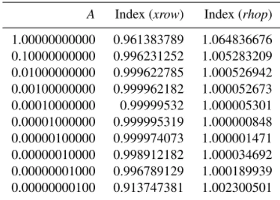
All input variables in the model should pass the TLM val-idation. There are many input variables in the model, but as the space of this paper is limited, we only choose two rep-resentative variables and provide the validation results here. For instance, the concentration value of pollutants (xrow) and the particle’s wet radius (rhop) are tested separately. The per-turbation value is set at 0.001 times the basic value forxrow
or rhop, the perturbation value of other variables is set to zero, and the decreasing ratio a is reduced to 0.1 ratio ev-ery time. The validation results are displayed in Table 1, from which it can be seen that the index value approaches 1.0 with decreasing a. Whena approaches zero, the index value slowly shifts away from 1.0 again; thus, the graph has a parabolic shape. This phenomenon is attributed to the ma-chine rounding error, as mentioned above.
2.2.4 Validation of the adjoint model
After all tangent linear codes have passed the testing, the ad-joint codes can be tested on the basis of the TLM. The adad-joint codes and the tangent linear codes need to satisfy Eq. (5) for all possible combinations of X andY. In Eq. (5), L repre-sents the tangent linear process andL∗ the adjoint process.
Table 1.Validation results of the tangent linear model.
A Index (xrow) Index (rhop)
1.00000000000 0.961383789 1.064836676 0.10000000000 0.996231252 1.005283209 0.01000000000 0.999622785 1.000526942 0.00100000000 0.999962182 1.000052673 0.00010000000 0.99999532 1.000005301 0.00001000000 0.999995319 1.000000848 0.00000100000 0.999974073 1.000001471 0.00000010000 0.998912182 1.000034692 0.00000001000 0.996789129 1.000189939 0.00000000100 0.913747381 1.002300501
To simplify the testing process, the adjoint input is the tan-gent linear output:Y=L(X). Thus, the above equation can be expressed as
(∇F·dX,∇F·dX)=(dX,∇TF (∇F·dX)). (11) By substituting dX into the tangent linear codes, the output value∇F·dXcan be obtained and the left part of the equation can be computed. Then, taking∇F·dX as the input of the adjoint codes, we obtain its output value∇TF (∇F·dX)and calculate the right part of the equation. As long as the resulted equation holds (within the error range), the constructed ad-joint model is validated.
Considering pollutant concentration variable xrow as an example, a smallxrow perturbation is input randomly, and the perturbation of other variables is set to zero. The pertur-bation value is taken as the tangent linear input. Then, we run the tangent linear codes once to obtain the value of the tan-gent linear output, and determine the inner product in the left side of Eq. (11). Next, we take the tangent linear output as the input of adjoint codes, run the adjoint codes once, and obtain the sensitivity value. Then, we use this value and the initial pollutant concentration perturbation to calculate the value of the right side of Eq. (11). In this calculation, it is important to keep the basic state value when doing the test, so that the tangent linear codes are consistent with the basic state of the adjoint codes. Otherwise, the calculated results will have no meaning. Assuming the result of the left part of the equa-tion is denoted as “VALTGL”, while that of the right part is “VALADJ”, the validation results are presented in Table 2.
Table 2.Validation results of the adjoint model.
Integral step VALTGL VALADJ
1 0.253071834334799587×10⁻¹¹ 0.253071834334799587×10⁻¹¹ 2 0.138781684963437701×10⁻⁷ 0.138781684963437635×10⁻⁷ 3 0.197243288646595624×10⁻⁶ 0.197243288646595703×10⁻⁶ 4 0.285995663142418833×10⁻⁶ 0.285995663142418833×10⁻⁶ 5 0.138094513716334626×10⁻⁶ 0.138094513716334599×10⁻⁶ 6 0.158774915826234477×10⁻⁶ 0.158774915826234609×10⁻⁶ 7 0.205383106884893541×10⁻⁶ 0.205383106884893673×10⁻⁶ 8 0.113356629291541069×10⁻⁶ 0.113356629291540963×10⁻⁶ 9 0.151566991405230902×10⁻⁶ 0.151566991405230823×10⁻⁶ 10 0.174929034468917025×10⁻⁶ 0.174929034468917104×10⁻⁶ 11 0.333573941572600298×10⁻⁶ 0.333573941572600616×10⁻⁶ 12 0.185912861066765391×10⁻⁶ 0.185912861066765523×10⁻⁶
Figure 1.Flow chart of GRAPES–CUACE, aerosol adjoint, and the flowchart of the parameters transmission process.
considered within the permitted range. As a result, all model variables passed the adjoint testing.
2.2.5 Operation flow of the GRAPES–CUACE aerosol adjoint model
After each part of the assembled TLM and the adjoint model were verified, the GRAPES–CUACE aerosol adjoint model was constructed. The structures and parameters flowchart is shown in Fig. 1. ADJ is short for adjoint; Xn and Xn+1 represent model parameters after n and n+1 GRAPES– CUACE integral time steps, respectively;Xn∗andX∗2 repre-sentXn’s adjoint∂J /∂XnandX2’s adjoint∂J /∂X2, respec-tively, where J is the objective function; ∂J /∂X are forc-ing terms; structures and variables in solid line frames are related to the forward simulation; and structures and vari-ables in dashed frames relate to the adjoint backward sim-ulation. In addition, as GRAPES–CUACE is an online at-mospheric chemistry modeling system, the aerosol transport processes are extracted from GRAPES. Therefore, a process called aerosol-related transport adjoint is presented in Fig. 1. When operating, the forward GRAPES–CUACE simula-tion should be run first to save the basic-state values of the unequilibrated variables in checkpoint files. Intermediate
val-ues are recalculated or saved in stack during the adjoint in-tegration. Then, the saved basic-state values during the for-ward integration and the forcing terms are used as inputs for the adjoint backward simulation.
2.3 Sensitivity analysis
To perform the sensitivity analysis and solve environmen-tal optimization problems, we usually take into account vari-ous factors, including air quality standards, economic losses, health benefits, the emissions reduction enforceable ratio range, and suitable locations for factories. Hence, a reason-able evaluation functionJ is needed, which includes one or several of the above factors as independent variables and/or as controlling conditions. In the adjoint method, such a func-tion is called the objective funcfunc-tion. We can define various types of objective functions based on different purposes. An objective function is always a function of the model output
Y, and may be simply denoted asJ=J (Y). The adjoint in-put, also called the forcing term (Fig. 1), is the gradient ofJ
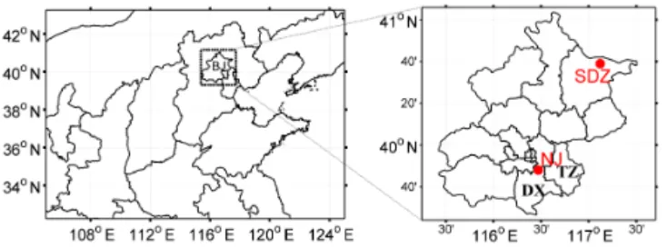
Figure 2. Left: model domain settings; right: the locations of Nanjiao (NJ) and Shangdianzi (SDZ) observation sites and the Tongzhou (TZ) and Daxing (DX) districts.
The principle application of the adjoint model is sensitivity analysis, and all its other applications may be considered to derive from it (Errico, 1997). In this research, J is defined as the concentration of the investigated pollutant when the pollution is greatest. Then, the inverse adjoint method can be used to locate where and when the emissions should have the greatest influence (time periods and regions with relatively larger sensitivity coefficients).
Because of its high efficiency in calculating sensitivity (or gradient), the adjoint model plays an important role in opti-mization problems. For example, in emission inventory op-timization problems, J is often defined as the discrepancy between the simulated and observed values. Running the ad-joint model once, the gradients (sensitivity) of the objec-tive function to the emission amount can be obtained, and then, by using the gradient information iteratively, the opti-mal emission intensity can be determined. In this study, op-timization problems were not carried out.
2.4 Model setup
In this study, the GFS reanalysis data, which are collected six times a day with 1◦×1◦resolution, are used as the initial and
boundary conditions in the GRAPES–CUACE modeling sys-tem, and INTEX-B2006 (0.5◦×0.5◦) is used as the emission
source. With a horizontal resolution of 0.5◦×0.5◦, the
sim-ulation domain covers northeast China (105–125◦E, 32.25– 42.25◦N), as shown in Fig. 2. Our analysis mainly focuses on the Beijing–Tianjin–Hebei (BTH) region. The entire sim-ulation period is from 20:00 BT (Beijing time) 28 June 2008 to 20:00 BT 4 July 2008; the first 72 h are regarded as the spin-up time.
2.5 Observations
The data used in this paper were obtained from the Bei-jing Meteorological Observatory Nanjiao station and Shang-dianzi station. The Nanjiao station (NJ; 39.8◦N, 116.47◦E) is located in the atmospheric observation test base in the southern suburb of Beijing. It is next to the Beijing urban area in the north and close to Fifth Ring Road in the south, where the traffic flow is relatively great. The Shangdianzi station (SDZ; 40.65◦N, 117.12◦E) is at the village
Shang-dianzi of Miyun County in northeastern Beijing. This sta-tion is a regional atmospheric background stasta-tion, around which there is no obvious industrial pollution and few hu-man activities, i.e., it represents a better ecological environ-ment. The locations of the two stations are shown in Fig. 2. Magee AE31 black carbon monitoring instruments are op-erated in both stations, with a 5 min sampling frequency (http://www.mageesci.com/). The hourly average BC con-centrations were calculated from these 5 min data.
3 Results and discussion
BC is an important component of atmospheric aerosols. It is emitted directly into the atmosphere predominantly during combustion (Seinfeld and Pandis, 2006). Its sources include anthropogenic and natural emission sources. Natural sources (e.g., volcanic eruption and forest fires) are occasional and regional, contributing little to the long-term background BC concentration in the atmosphere (Parungo et al., 1994). Com-paratively, many human activities increase the concentra-tion of BC aerosols; therefore, anthropogenic sources are the primary sources of BC. Streets et al. (2001) and Cao et al. (2006) noted that the vast majority of BC emissions in China are produced by the untreated raw coal, honeycomb briquettes, and biomass fuels that people use in their daily lives.
BC is the main light-absorbing aerosol species; it alters the radiative properties of other aerosols with which it is mixed. In addition, it may also affect cloud formation and precip-itation (Hakami et al., 2005), reduce crop production, de-crease visibility, and harm human health. In one word, BC plays an essential role in atmospheric radiative forcing, cli-mate change, and air quality evaluation.
3.1 High BC concentration episode and model validation
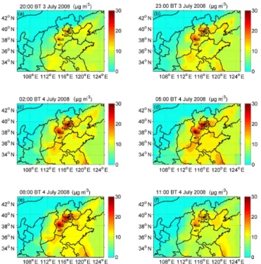
The simulated ground BC concentration distributions from 20:00 BT 3 July to 11:00 BT 4 July are shown in Fig. 3. These six graphs illustrate the formation and transportation processes of this high BC concentration episode over Bei-jing. At 20:00 BT 3 July, two small spots of high BC con-centrations appeared around Shijiazhuang (SJZ; 114.48◦E, 38.03◦N) and southern Beijing. At 23:00 BT 3 July, these
two high BC concentration spots were obviously enlarged and almost connected, extending to northern Xingtai (XT; 114.48◦E, 37.05◦N), eastern Baoding (BD; 115.48◦E,
Figure 3. BC concentration distribution at ground level (Unit: µg m−3).
BC concentration over Beijing remains at a relatively higher level.
Figure 4 shows the hourly variation of ground-level BC concentration in Beijing. It is easy to notice that during the first 2 simulated days, the BC concentration reached its peak at approximately 02:00 BT on 2 and 3 July, and its lowest value at approximately 15:00 BT on the same days. Thus, the absolute BC concentration in this case appears to be af-fected by the diurnal height variation of the boundary layer, atmospheric stability, and diffusion conditions. On the con-trary, the highest BC concentration on 4 July (15.7 µg m−3)
was recorded at 11:00 BT, perhaps because, on that day, the atmospheric conditions were more stable, and the pollutant diffusion was unsatisfactory, thus leading to BC accumula-tion.
The model results are compared with the above observa-tion data in Fig. 5. The correlaobserva-tion coefficients of the simu-lated and the observed BC concentrations at Shangdianzi and Nanjiao stations are 0.65 and 0.54, respectively. Therefore, the general variation trends of the simulated and observed BC concentrations are consistent. However, the simulated BC concentration values are greater than the corresponding observed values at both stations, with MRs / o (the mean ra-tio of the simulated to the observed) equal to 2.2 and 6.4 at Nanjiao and Shangdianzi stations, respectively. Overesti-mates are also reflected by the positive value of MFB (mean functional bias; Boylan and Russell, 2006) at the two stations (60.5 % at NJ station and 112.3 % at SDZ station). The MFEs (mean functional errors) are 60.5 and 115.6 % at NJ station and SDZ stations, respectively. As SDZ station is a regional
Figure 4.Hourly variation of simulated ground BC concentration over the Beijing municipality.
background station with no obvious industrial pollution and few human activities, the observational concentrations there are very small. Using the mean concentration over a coarse model grid (0.5◦×0.5◦) to represent BC concentrations at the background station directly leads to overestimation. The same reason applied to overestimation at NJ station. Previ-ous studies (Zhou et al., 2012; Wang et al., 2015a, b; Jiang et al., 2015) based on the GRAPES–CUACE modeling system have showed the reliability of the model very well. Overall, we consider the model results acceptable.
3.2 Objective function and sensitivity coefficient definitions
As mentioned above, the adjoint method can provide infor-mation about the influences of location-specific sources on the objective function. To determine the area and the time pe-riod when the most important emission sources fed the high-est BC concentration over Beijing as recorded at 11:00 BT 4 July 2008 (Fig. 4), we define the objective function J
as the average BC concentration over Beijing at 11:00 BT 4 July 2008.
The adjoint input, also regarded as a forcing term, is
∂J /∂C.Crepresents the pollutant concentration, such as the BC concentration, at the objective time. The direct output from the adjoint model is the gradient ofJ with respect to any model parameter var:∂J /∂var. If var is the hourly grid-ded offline emissions intensityq, then∂J /∂q directly con-nects the objective functionJ with emissions. The larger an emission source’s∂J /∂qis, the greater its influence is onJ. However, this kind of sensitivity definition does not reflect the absolute influence of certain emission sources. For exam-ple, for an emission source with relatively large∂J /∂q, but quite smallq, its actual influence will be negligible. There-fore, we define the emission sensitivity coefficient8as
8=q∂J
Figure 5. Comparisons of observed and modeled hourly BC concentrations at Nanjiao and Shangdianzi stations from 20:00 1 July 2008 to 19:00 4 July 2008. Statistical parameters used are mean functional bias (MFB), mean functional error (MFE), mean value of the simulated (Ms), mean value of the observed (Mo)and Mean ratio of the simulated to the observed (Ms / o)
In this way, the emission sensitivity coefficient 8 has the same unit with J and has a specific physical meaning. In a given area, the BC emissions’ influence onJ increases with the sensitivity coefficient value. If the BC emissions is re-duced byN %, the value ofJ decreases byN%·8, which means that the average BC concentration over Beijing at the objective time point also decreases byN%·8.
3.3 Distribution of adjoint sensitivity
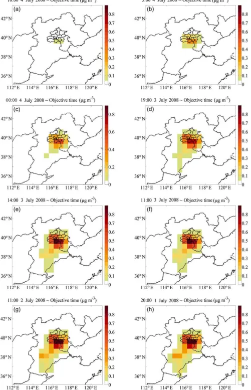
To control air quality, usually emissions are cut over a certain period, e.g., 1–3 days ahead of the predicted severe pollution day. Based on this practical concept, sensitivity coefficients at every model’s backward integral time step are added from the objective time point (highest BC concentration: 11:00 BT 4 July 2008) to a certain preceding time point, as illustrated in Fig. 6. Figure 6 shows a spatial–temporal cumulative effect from BC emissions to the objective functionJ.
As shown in Fig. 6, sensitivity coefficients accumulate along an inverse time series. When sensitivity coefficients from the previous hour until the objective time point are added, only the Tongzhou (TZ) and Daxing (DX) districts (locations of TZ and DX districts were shown in Fig. 2) in Beijing have sensitivity coefficients of 0.05–0.1 µg m−3. When sensitivity coefficients are added for the last 6 h, the in-fluential area is remarkably enlarged, with a maximum value of 0.3–0.4 µg m−3. As the hours ahead of the objective time points are increased, this influenced area is continually en-larged and intensified. When it reaches the 16 h period, as shown in Fig. 6d, the more critical area expands to Lang-fang and Baoding of the Hebei province, and the maximum value is approximately 0.7 µg m−3. This indicates that reduc-ing BC emission at a ratio ofN% from 19:00 BT 3 July to the objective time point over this grid cell could result in an average N%·0.7 µg m−3decrease of the BC concentra-tion over Beijing (objective region), at 11:00 BT 4 July 2008 (objective time point). However, along with this
accumula-Table 3.Information on the four emission reduction regions.
Region Number of grid cells Area (km2)
BTH 105 318 000
BJ 10 30 000
InR-1 7 21 000
InR-2 17 51 000
tion procedure, the expansion of the influential region scope and the increase in its sensitivity coefficients begin to slow down. Only a tiny difference between 24 h of accumulation (Fig. 6f) and 48 h of accumulation (Fig. 6g) is observed. This phenomenon reflects that emissions from 11:00 BT 2 July to 11:00 BT 3 July have little influence on J. When a heavy pollution event needs to be controlled by reducing emissions, the time period with the most significant influence should be scientifically determined in order to cut emissions both effec-tively and economically.
3.4 Time series of sensitivity coefficients in different regions
Adjoint sensitivity analysis is a powerful complement to for-ward methods. While forfor-ward techniques are source-based, backward methods provide receptor-based sensitivity infor-mation. Under this conception, we use the adjoint method to locate the most influential emission sources area and the most influential emission time period.
Four types of regions are defined according to administra-tive division and the sensitivity coefficients distribution (Ta-ble 3 and Fig. 7). BTH refers to the administrative Beijing– Tianjin–Hebei region, which covers 105 grid cells and is ap-proximately 318 000 km2; BJ represents administrative Bei-jing, which contains 10 grid cells and covers an area of around 30 000 km2. InR-1 (Influential Region 1) has 7 grid cells, occupying about 21 000 km2, which is smaller than that of BJ, whose sensitivity coefficient values are obviously larger than others; InR-2 (Influential Region 2) covers InR-1 and 10 more grid cells with secondary large coefficient val-ues, having 17 grid cells in total and covering approximately 51 000 km2.
Figure 6.Cumulative sensitivity coefficient distribution. Panels(a–e)are 1, 6, 11, 16, and 21 h cumulative sensitivity coefficients. Panels
(f–g)are 24 and 48 h cumulative coefficients, and(h)is the last backward simulation time step.
In Fig. 8a, the sensitivity coefficients of BTH, InR-1, and BJ reach their peak values at 18:00 BT 3 July, whereas that InR-2 is maximized at 17:00 BT 3 July. Afterward, they all decrease sharply along a backward time sequence. This phe-nomenon indicates that the impact of emissions on J be-gins to decrease along the inverse time sequence axis before 17:00–18:00 BT 3 July, about 17–18 h ahead of the most
Table 4.18 h (17:00 BT 3 July–11:00 BT 4 July) cumulative SC and SC/Grid over the four emission reduction regions.
Regions
SC BTH (µg m−3) BJ (µg m−3) InR-1 (µg m−3) InR-2 (µg m−3) InR-2/BTH InR-1/BJ
SC 7.3 3.5 4.0 5.9 0.8 1.2
SC/Grid 0.07 0.35 0.58 0.35 5.0 1.6
SC: sensitivity coefficient. SC/Grid: sensitivity coefficient per simulation grid.
Figure 7. Different influential regions. BTH: red dashed frame; InR-1: blue dashed frame; InR-2: pinkish red solid frame; object region: yellow shadow.
Then, we compare the preceding 18 h cumulative sensi-tivity coefficients, from 17:00 BT 3 July to 11:00 BT 4 July, for the above four regions (Table 4), given that the sensi-tivity coefficient on 17:00 BT 3 July is still relatively high (for BTH, InR-1, and BJ). From Table 4, the simulated SC (sensitivity coefficient) of BTH is 7.3 µg m−3, meaning that a reduction of N% BC emissions over BTH will cause an
N%·7.3 µg m−3 decrease of average BC concentration in Beijing on 11:00 BT 4 July. In general, it is obvious that re-ducing emissions over the entire BTH region will contribute most positively to air quality control in Beijing, followed by InR-2, InR-1, and BJ. However, from the four regions, the SC/Grid (sensitivity coefficient per grid) value is the largest in InR-1. Therefore, cutting the emissions of InR-1 has the most obvious effectiveness in decreasing the BC concentra-tion in Beijing. The SC/Grid of BTH is the smallest, and InR-2 is equivalent to BJ with intermediate concentrations. BTH covers an area which is 6.2 times that of InR-2, but the SC and SC/Grid of Inr-2 are 80 % and 5.0 times of BTH (Ta-ble 4). A similar phenomenon is found between BJ and InR-1. InR-1 accounts for only 70 % of the BJ area, but the SC and SC/Grid of InR-1 are 1.2 and 1.6 times that of BJ.
4 Conclusions
In this study, based on the adjoint theory and methods, we constructed and tested an adjoint model for an aerosol mod-ule of the atmospheric chemical model GRAPES–CUACE.
Figure 8. (a)Sensitivity coefficients at each 5 min integration time step along inverse time sequence;(b)cumulative sensitivity coeffi-cients along inverse time series.
Developing the GRAPES–CUACE aerosol adjoint model in-cluded constructing and validating the tangent linear and the adjoint models of the three parts involved in the GRAPES– CUACE aerosol module: CAM, interface programs, and the aerosol transport processes. Meanwhile, strict mathematical validation schemes for the tangent linear and the adjoint models were carried out for all input variables. After the as-sembled tangent linear and the adjoint models for each part were verified, the adjoint model of the GRAPES–CUACE aerosol was constructed. At the same time, the GRAPES– CUACE model and its aerosol adjoint were adopted to per-form a numerical simulation and a receptor–source sensitiv-ity test. Compared with the BC aerosol observations from the Nanjiao and Shangdianzi stations, the hourly trends of BC concentration estimated through the present model were similar, with correlation coefficients 0.65 and 0.54, respec-tively.
(about 17–18 h) had a much greater influence than emissions emitted earlier than that.
The BC adjoint sensitivity results presented here could help design efficient haze control schemes using the adjoint method. It is found that to increase the emission reduction efficiency, influential regions should be located scientifically (e.g., according to the adjoint sensitivity coefficients distri-bution) rather than based on administrative divisions.
5 Code availability
We used the GRAPES–CUACE as distributed by the Numer-ical Weather Prediction Center of Chinese Meteorology Ad-ministration (http://nwpc.cma.gov.cn) together with the Insti-tute of Atmospheric Composition of the Chinese Academy of Meteorological Sciences (http://www.cams.cma.gov.cn). The model was run on an IBM PureFlex System (AIX) with an XL Fortran Compiler. The CUACE–ADJ code can be re-quested from the corresponding author or downloaded as a Supplement to this article.
The Supplement related to this article is available online at doi:10.5194/gmd-9-2153-2016-supplement.
Acknowledgements. This study was supported by the National Natural Science Foundation of China (41575151), the Na-tional Science-Technology Support Program (2014BAC16B03), and the CMA Innovation Team for Haze-fog Observation and Forecasts. We appreciate Lin Zhang, Feng Liu, Qiang Cheng, Hongliang Zhang, and Min Xue for providing technical support in adjoint model construction. Thanks are also owed to the developers of the GRAPES–CUACE aerosol model. The authors are indebted to the anonymous referees for their valuable comments.
Edited by: J. Annan
References
Boylan, J. W. and Russell, A. G.: PM and light extinction model performance metrics, goals, and criteria for three di-mensional air quality models, Atmos. Environ., 40, 4946–4959, doi:10.1016/j.atmosenv.2005.09.087, 2006.
Cacuci, D. G.: Sensitivity theory for nonlinear systems. I. Non-linear functional analysis approach, J. Math. Phys., 22, 2794, doi:10.1063/1.525186, 1981a.
Cacuci, D. G.: Sensitivity theory for nonlinear systems. II. Exten-sions to additional classes of responses, J. Math. Phys., 22, 2803, doi:10.1063/1.524870, 1981b.
Cao, G., Zhang, X., Wang, Y., Che, H., and Chen D: Inventory of Black Carbon Emission from China, Advances in Climate Change Research, 2, 259–264, 2006 (in Chinese).
Chen, H., Hu, F., Zeng, Q., and Chen, J.: Some Practical Problems of Optimizing Emissions from Pollution Sources in Air, Climatic and Environmental Research, 3, 163–172, 1998 (in Chinese). Cheng, Q., Zhang, H., and Wang, B.: Algorithms of Automatic
Dif-ferentiation, Mathematica Numerica Sinica, 33, 15–36, 2009 (in Chinese).
Elbern, H., Schmidt, H., Talagrand, O., and Ebel, A.: 4D-variational data assimilation with an adjoint air quality model for emission analysis, Environ. Model. Softw., 15, 539–548, 2000.
Errico, R. M.: What is an adjoint model, B. Am. Meteorol. Soc., 78, 2577–2591, 1997.
García-Chan, N., Alvarez-Vázquez, L., Martínez, A., and Vázquez-Méndez, M.: On optimal location and management of a new in-dustrial plant: Numerical simulation and control, J. Frankl. Inst., 351, 1356–1371, doi:10.1016/j.jfranklin.2013.11.005, 2013. Gong, S. L., Barrie, L. A., Blanchet, J.-P., Salzen, K. v., Lohmann,
U., Lesins, G., Spacek, L., Zhang, L. M., Girard, E., and Lin, H.: Canadian Aerosol Module: A size-segregated simulation of atmospheric aerosol processes for climate and air quality models, 1, Module development, J. Geophys. Res., 108, 4007, doi:10.1029/2001JD002002, 2003.
Hakami, A., Henze, D. K., and Seinfeld, J. H.: Adjoint inverse mod-elling of black carbon during the Asian Pacific Regional Aerosol Characterization Experiment, J. Geophys. Res., 110, D14301, doi:10.1029/2004JD005671, 2005.
Hakami, A., Henze, D. K., Seinfeld, J. H., Singh, K., Sandu, A., Kim, S., Byun, D., and Li, Q.: The adjoint of CMAQ, Environ. Sci. Technol., 41, 7807–7817, 2007.
Henze, D. K., Hakami, A., and Seinfeld, J. H.: Development of the adjoint of GEOS-Chem, Atmos. Chem. Phys., 7, 2413–2433, doi:10.5194/acp-7-2413-2007, 2007.
Henze, D. K., Seinfeld, J. H., and Shindell, D. T.: Inverse model-ing and mappmodel-ing US air quality influences of inorganic PM2.5 precursor emissions using the adjoint of GEOS-Chem, At-mos. Chem. Phys., 9, 5877–5903, doi:10.5194/acp-9-5877-2009, 2009.
Jiang, C., Wang, H., Zhao, T., Li, T., and Che, H.: Modeling study of PM2.5pollutant transport across cities in China’s Jing–Jin– Ji region during a severe haze episode in December 2013, At-mos. Chem. Phys., 15, 5803–5814, doi:10.5194/acp-15-5803-2015, 2015.
Koo, J., Wang, Q., Henze, D. K., Waitz, I. A., and Barrett, S. R.: Spatial sensitivities of human health risk to intercontinen-tal and high-altitude pollution, Atmos. Environ., 71, 140–147, doi:10.1016/j.atmosenv.2013.01.025, 2013.
Liu, F.: Adjoint model of Comprehensive Air quality Model CAMx – construction and application, Peking University Post-doctoral Reseach Report, 2005.
Liu, F. and Hu, F.: Inversion of Diffusion on Coefficients And Effect of Related Difference Schemes, J. Appl. Meteorol. Sci., 14, 331– 338, 2003 (in Chinese).
Liu, F., Zhang, Y., Su, H., and Hu, J.: Adjoint Model of Atmospheric Chemistry Transport Model CAMx: Construction and Applica-tion, Acta Scientiarum Natruralium Universitatis Pekinensis, 43, 764–770, 2007 (in Chinese).
Marchuk, G.: Mathematical Models in Environmental Problems, New York: Elsevier Science Publishers, 1986.
with the oceans and continents, Izvestiya Atmospheric Oceanic Physics, 12, 279–284, 1976.
Pappin, A. J. and Hakami, A.: Source Attribution of Health Ben-efits from Air Pollution Abatement in Canada and the United States: An Adjoint Sensitivity Analysis, Environ. Health Persp., 121, 572–579, 2013.
Parungo, F., Nagamoto, C., Zhou, M. Y., Hansen, A. D. A., and Harris, J.: Aeolian transport of aerosol black carbon from China to the ocean, Atmos. Environ., 28, 3251–3260, 1994.
Paulot, F., Jacob, D. J., Pinder, R. W., Bash, J. O., Travis, K., and Henze, D. K.: Ammonia emissions in the United States, Eu-ropean Union, and China derived by high-resolution inversion of ammonium wet deposition data: Interpretation with a new agricultral emissions inventory (MASAGE_NH3), J. Geophys. Res.-Atmos., 119, 4343–4364, doi:10.1002/2013JD021130, 2014.
Resler, J., Eben, K., Jurus, P., and Liczki, J.: Inverse modeling of emissions and their time profiles, Atmospheric Pollution Re-search, 1, 288–295, doi:10.5094/APR.2010.036, 2010.
Sandu, A., Daescu, D. N., Carmichael, G. R., and Chai, T.: Ad-joint sensitivity analysis of regional air quality models, J. Com-put. Phys., 204, 222–252, 2005.
Seinfeld, J. H. and Pandis S. N.: Atmospheric Chemistry and Physics: From Air Pollution to Climate Change, 2nd Edn., John Wiley & Sons, Inc., 628–633, 2006.
Sfetsos, A., Vlachogiannis, D., and Gounaris, N.: An Investigation of the Factors Affecting the Ozone Concentrations in an Urban Environment, Atmos. Clim. Sci., 3, 11–17, 2013.
Skiba, Y. and Parra-Guevara, D.: Industrial pollution transport. Part 1. Formulation of the problem and air pollution estimates, Envi-ron. Model. Assess., 5, 169–175, 2000a.
Skiba, Y. and Parra-Guevara, D.: Industrial pollution transport. Part 2. Control of industrial emissions, Environ. Model. Assess., 5, 177–184, 2000b.
Skiba, Y. N. and Davydova-Belitskaya, V.: Air pollution estimates in Guadalajara City, Environ. Model. Assess., 7, 153–162, 2002. Skiba, Y. N. and Davydova-Belitskaya, V.: On the estimation of im-pact of vehicular emissions, Ecol. Model., 166, 169–184, 2003. Streets, D., Gupta, S., and Waldho, S.: Black carbon emissions in
China, Atmos. Environ., 35, 4281–4296, 2001.
Turner, M.: Inverse Modeling of NOx and NH3Precursor Emis-sions Using the Adjoint of CMAQ, Research Prelim Report, De-partment of Mechanical Engineering, University of Colorado, 2010.
Wang, H., Gong, S. L., Zhang, H. L., Chen, Y., Shen, X. S., Chen, D. H., Xue, J. S., Shen, Y. F., Wu, X. J., and Jin, Z. Y.: A new-generation sand and dust storm forecasting sys-tem GRAPES-CUACE/Dust: Model development, verification and numerical simulation, Chinese Sci. Bull, 54, 3878–3891, doi:10.1007/s11434-009-0481-z, 2009.
Wang, H., Shi, G. Y., Zhang, X. Y., Gong, S. L., Tan, S. C., Chen, B., Che, H. Z., and Li, T.: Mesoscale modelling study of the in-teractions between aerosols and PBL meteorology during a haze episode in China Jing–Jin–Ji and its near surrounding region – Part 2: Aerosols’ radiative feedback effects, Atmos. Chem. Phys., 15, 3277–3287, doi:10.5194/acp-15-3277-2015, 2015a. Wang, H., Xue, M., Zhang, X. Y., Liu, H. L., Zhou, C. H., Tan, S.
C., Che, H. Z., Chen, B., and Li, T.: Mesoscale modeling study of the interactions between aerosols and PBL meteorology during a haze episode in Jing–Jin–Ji (China) and its nearby surrounding region – Part 1: Aerosol distributions and meteorological fea-tures, Atmos. Chem. Phys., 15, 3257–3275, doi:10.5194/acp-15-3257-2015, 2015b.
Wang, X.: Toward the Objective Analysis, Four-Dimensional As-similation and Adjoint Method, Journal of PLA University of Science and Technology, 1, 67–74, 2000 (in Chinese).
Xue, J. and Chen, D.: Scientific Design and Application of Numer-ical Predicting System GRAPES, Science Press, Beijing, 2008. Zhai, S. X.: Development of the adjoint of GRAPES-CUCAE
aerosol module and model application to air pollution optimal control problems, MSc diss., Chinese Academy of Meteorologi-cal Sciences, 2015.
Zhang, L., Jacob, D. J., Kopacz, M., Henze, D. K., Singh, K., and Jaffe, D. A.: Intercontinental source attribution of ozone pollu-tion at western U.S. sites using an adjoint method, Geophys. Res. Lett., 36, L11810, doi:10.1029/2009gl037950, 2009.
Zhao, S., Pappin, A. J., Morteza Mesbah, S., Joyce Zhang, J., Mac-Donald, N. L., and Hakami, A.: Adjoint estimation of ozone cli-mate penalties, Geophys. Res. Lett., 40, 5559–5563, 2013. Zhou, C. H., Gong, S. L., Zhang, X. Y., Liu, H. L., Xue,
M., Cao, G. L., An, X. Q., Che, H. Z., Zhang, Y. M., and Niu, T.: Towards the improvements of simulating the chem-ical and optchem-ical properties of Chinese aerosols using an on-line coupled model – CUACE/Aero, Tellus B, 64, 18965, doi:10.3402/tellusb.v64i0.18965, 2012.
Zhu, J. and Zeng, Q.: A mathematical theory frame for atmospheric pollution control, Science China (D), 32, 864–870, 2002. Zhu, J., Zeng, Q., Guo, D., and Liu, Z: Optimal control of