Adv. Sci. Res., 3, 105–112, 2009 www.adv-sci-res.net/3/105/2009/
©Author(s) 2009. This work is distributed under the Creative Commons Attribution 3.0 License.
Advances in
Science and
Research
8th
EMS
Annual
Meeting
and
7th
Eur
opean
Confer
ence
on
Applied
Climatolo
gy
2008
Efficient high-resolution 3-D interpolation of
meteorological variables for operational use
C. Lussana1, M. R. Salvati1, U. Pellegrini1, and F. Uboldi2 1ARPA Lombardia, Milano, Italy
2Consultant, Novate Milanese, Italy
Received: 19 December 2008 – Revised: 7 June 2009 – Accepted: 8 June 2009 – Published: 5 August 2009
Abstract. In recent years, the use of mesoscale meteorological network data has been growing. An Optimal Interpolation (OI) method is used to interpolate on a regular grid the hourly averaged values of temperature, relative humidity, wind vector, atmospheric pressure, and hourly cumulated precipitation. For all variables, except precipitation, the background (i.e. first guess) information is obtained by detrending the observations using the geographical parameters. For precipitation, the M. Lema radar-derived best estimate of precipitation rate at the ground is used. The characteristics of the OI schemes are shown in several test cases using data from ARPA Lombardia’s mesoscale meteorological network. Finally, a quantitative diagnostics for temperature and relative humidity is carried out by using Cross Validation (CV) scores computed with large sets of data.
1 Introduction
This document describes a spatial interpolation scheme based on Optimal Interpolation (OI; Gandin, 1963) applied to the data collected by a mesoscale meteorological network. OI is a method widely used in meteorology and climatology and it is based on a linear combination of the observed values with a background field weighting their respective uncertain-ties. For a review of OI and its comparison with other data interpolation techniques see for example Daley (1991) and Kalnay (2003). In the presented work, the analyzed fields are mostly intended as support to nowcasting and forecasting in an operational meteorological centre. Forecasters require easy access to several different variables to gain better insight into meteorological phenomena: for this reason the OI is ap-plied to hourly averaged observations of temperature, wind, relative humidity, pressure, and to the hourly cumulated pre-cipitation.
The observing system is ARPA Lombardia’s mesoscale meteorological network, managed by the local public weather service. The meteorological network is character-ized by a high space and time resolution of observations (au-tomatic stations), but with strong inhomogeneities in sensors’ distribution. As an example, Fig. 1 shows raingauges and anemometers observation locations. Lombardy itself is
char-Correspondence to:C. Lussana
acterized by a very complex orography and by different land uses: the representativity component of the observational er-ror plays an important role and must be properly handled.
The interpolation is performed over a regular grid. The spatial domain measures roughly 200 km×200 km. A grid resolution of 1.5 km has been chosen: it is the coarser reso-lution that can be used without having significant differences between grid and station elevation. It is worth remarking that it is the grid resolution that accounts for most of the to-pographic detail of the analysis maps, and that the grid reso-lution is higher than the observation network resoreso-lution.
About three years of operational use have proven the algo-rithm to be efficient (in using computer resources) and stable (with respect to the observing system’s anomalies or mal-functionings). Furthermore, the OI procedures themselves have revealed some of the network’s problems.
Figure 1. Orography and station locations in the domain. Trian-gles: raingauges. Circles: anemometers. The bold black line is the administrative boundary. The inset shows the geographical loca-tion of Lombardy (Italy), longitude 8.5 to 11.5◦E, latitude 44.6 to
45.7◦N.
2 Optimal Interpolation schemes
The statistical interpolation scheme used for this work is de-scribed in Uboldi et al. (2008), where it is applied to temper-ature and relative humidity. Generally, OI schemes use an observation independent background field. This scheme uses instead a 3-D background obtained by observations detrend-ing; this field is representative of the larger scale captured by the network. The present manuscript describes the evolution of the OI scheme and its application to other meteorological quantities. It is worthwhile remarking that the OI scheme described in Uboldi et al. (2008) can also make use of an independent background, as it is done here for precipitation. Table 2 summarizes the choices made in OI implementa-tion for the variables treated in this work. All the spatial cor-relation functions used are isotropic except for the improved OI algorithm for temperature. The last three columns of Ta-ble 2 report the values forDh,Dzandε2. The de-correlation length scales in the horizontal direction and in the vertical di-rection, DhandDz respectively, are used in the background error spatial correlation functions to determine the volume
Figure 2.20 January 2006, 12:00 LT (Local Time=UTC+1). Tem-perature analysis (unit◦C). The isoline 0◦C is shown in gray; the
white contours mark urban areas.
influencing the analysis at each point inside the domain. The
ε2parameter is defined as the ratio between observation and background uncertainties.
The choices regarding the background must be variable dependent, and are also summarized in Table 2. In the context of statistical interpolation, precipitation must be re-garded as a variable apart from the others because of its specific statistical properties. The OI implementation used in this work combines raingauge measurements and the M. Lema radar-derived Best Estimate of Precipitation rate at the ground (BEP; Joss et al., 1998). Due to the extremely dis-continuous nature of the precipitation field, the availability of a background from radar data is very important in recon-structing the analysis field. An effort is made to integrate the two sources of information without degrading them.
C. Lussana et al.: High-resolution interpolation of meteorological data 107
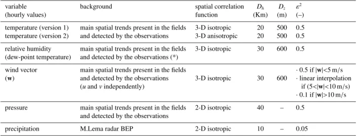
Table 1.Summary of OI implementations for each variable. For a detailed description of the parameters see also Uboldi et al. (2008). Dh andDzare the de-correlation length scales in the horizontal direction and in the vertical direction used in the spatial correlation functions;
ε2 is the estimated ratio between the variances of observation and background errors (for wind intensities between 5 and 10 m s−1 theε2
value is interpolated linearly between 0.1 and 0.5). A dew-point temperature observation (*) is obtained combining temperature and relative humidity observed at the same station.
variable background spatial correlation Dh Dz ε2
(hourly values) function (Km) (m) (–)
temperature (version 1) main spatial trends present in the fields 3-D isotropic 20 500 0.5 temperature (version 2) and detected by the observations 3-D anisotropic 20 500 0.5
relative humidity main spatial trends present in the fields 3-D isotropic 30 600 0.5 (dew-point temperature) and detected by the observations (*)
wind vector main spatial trends present in the fields ·0.5 if|w|<5 m/s (w) and detected by the observations 3-D isotropic 30 600 ·linear interpolation
(uandvindependently) if (5<|w|<10 m/s)
·0.1 if|w|>10 m/s
pressure main spatial trends present in the fields 2-D isotropic 40 – 0.5 and detected by the observations
precipitation M.Lema radar BEP 2-D isotropic 10 – 0.05
information. Besides, a model-independent analysis can be a convenient choice for studying network’s characteristics, and in the case of model verification studies.
In Uboldi et al. (2008) the OI implementation for temper-ature and relative humidity is described. With respect to that work, here, in order to account for the urban heat island ef-fect, some anisotropy is introduced in the spatial correlation functions for temperature. Urban (grid point/station) loca-tions are decorrelated from non-urban localoca-tions depending on the land use in their surroundings. In principle, such a procedure can be extended to other variables.
The interpolation scheme constrains the wind vector to be locally tangent to the grid orography, by making its nor-mal component vanish. The background field is obtained by detrending the zonal and the meridional wind observations independently. Finally, wind observations with a module greater than 10 m s−1 are assumed to be more reliable than
weak wind observations, influenced by meandering.
For precipitation, the assumption of Gaussian pdf for ob-servation and background errors, implicit in the OI, is very far from reality. In particular, when the observations or the background have zero value then the analyzed field must be exactly zero, while if the reported values for observations or background are positive then the interpolation scheme must always reconstruct positive analysis values. The interpola-tion procedure must be able to correctly describe both be-haviours. For each grid point, the Integral Data Influence (IDI; Uboldi et al., 2008) value computed by only using zero precipitation observations is compared with the IDI value computed by only using positive precipitation observations. Where the “zero-rain” IDI prevails, the analysis value is set to zero. Elsewhere, positive values are interpolated from (positive) observations.
All observations of temperature, relative humidity, wind and pressure are hourly averages, precipitation observations are hourly cumulated values.
3 Test cases
The characteristics of the interpolation scheme are shown by using test cases that present strong gradients in the variables’ fields. Strong gradients stress the interpolation scheme, ev-idencing the spatial scales that it is able to reproduce. The meteorological situations chosen -a persistent fog situation, two foehn cases and two precipitation cases- are also relevant for civil protection and economical activities.
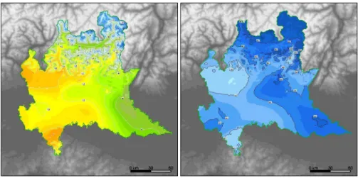
3.1 Fog in the Po Plain
This test case refers to a winter case of high pressure subsi-dence causing persistent fog in the Plain (see Fig. 3). The fog, of radiative origin, is associated with a marked ground-based inversion that is well reproduced in temperature and relative humidity fields as an intense gradient in the plain area. The correspondence between the limit of the cloudy area in the meteosat image, a completely independent source of information, and the gradients in the analyzed fields is sat-isfactory. The fields of wind and atmospheric pressure re-duced to the mean sea level, not shown here, exhibit the weak gradients expected in such a situation.
Figure 3.20 January 2006, 12:00 LT. Left: Temperature. Center: Meteosat-8 Channel 12 (HRV) image. Right: relative humidity (unit %). The temperature scale is the same as in Fig. 2.
Figure 4.21 January 2005, 12:00 LT. Left: temperature. Right: relative humidity. See Figs. 2 and 3 for temperature and relative humidity scales, respectively.
area, in the western part of the region. By integrating land use information in the OI scheme, it is possible to recognize and decorrelate urban from non-urban locations. The final effect can be seen by comparing the left panel in Fig. 3 with Fig. 2 in the Milan area. A careful inspection of the me-teosat picture shows better agreement with the field in Fig. 2, especially for the Milan area, and a quantitative diagnostics using Cross Validation (CV) scores confirms this qualitative evaluation.
3.2 Foehn cases
3.2.1 21 January 2005
The first case, well documented on-line (Eumetsat, 2008), refers to 21 January 2005. The Alps are under the influence
C. Lussana et al.: High-resolution interpolation of meteorological data 109
Figure 5. 12 March 2006, 08:00 LT. Left: wind vectors (unit m s−1; white boxes contain observations and mark station locations). Right:
pressure (reduced to the mean sea level; unit hPa).
3.2.2 12 March 2006
The meteorological situation for the second foehn case – 12 March 2006 – is similar to the previous one. However, in this case the eastern part of the region is still under the in-fluence of a cyclonic circulation. Very low temperature val-ues were observed in the mountain areas to the northeast, and light snowfall occurred during the morning in the south-eastern plain. As can be seen in Fig. 5, the wind field pat-tern is in agreement with the analyzed pressure gradient; the wind intensity maxima correctly correspond to the dry and warm areas in the temperature and relative humidity analysis (not shown here). It is worth remarking that all the variables are analyzed independently: their consistency is a qualitative confirmation that the OI does not introduce large errors.
3.3 Precipitation cases
The results for OI of cumulated precipitation are presented in two very different cases: a case of convective precipitation and a case of stratiform precipitation. Convective and strati-form precipitation have different spatial and temporal coher-ence, but in both cases the integrated field retains the good features of raingauges observations and post-processed radar background information. The realistic appearance of the 24 h cumulated fields also shows that any systematic error intro-duced by the interpolation algorithm must be of small am-plitude. In fact, even summing-up many precipitation fields, unrealistic features do not appear.
In order to show the characteristics of the integration of the available information, the precipitation analysis fields for the test cases chosen are compared with the OI of raingauges
observation only and with the M. Lema best estimate of pre-cipitation rate at the ground (Joss et al., 1998).
3.3.1 Convective precipitation
Convective precipitation is characterized by small horizontal scales and high vertical extension of the precipitating vol-ume. As can be seen in Fig. 6, in this case the radar estimate of the rain field (center panels) is more realistic than what can be obtained with raingauges only (leftmost panels). In the latter, the spatial pattern is clearly mainly determined by the station distribution and the symmetrical correlation func-tions. The analysis in the rightmost panels, integrating the two sources, maintain the radar’s realistic features.
By cumulating the analysis fields over 24 h, the peak of precipitation observed in the radar estimate is correctly con-served in the integrated map.
3.3.2 Stratiform precipitation
Figure 6. 24 August 2006. Convective precipitation case. The panels above show 1-h precipitation (23:00 LT; unit mm h−1) while panels
below show 24-h cumulated precipitation (unit mm day−1). Left: analysis field obtained by using raingauges only. Center: M. Lema
radar-derived best estimate of precipitation rate at the ground. Right: integration of both informational sources. The observed values reported in hourly analysis mark station locations.
4 Cross Validation scores
The CV score is routinely computed for each analysis time for temperature and relative humidity. The CV score repre-sents an estimate of the analysis error, based on the idea that each observation is used as an independent verification of the analysis field. The CV score distribution for temperature has been computed for the entire 2006: the overall median is 1.45◦C and the interquartile range is 0.50◦C. By group-ing stations accordgroup-ing to the IDI, stations belonggroup-ing to dense areas of coverage has a CV score distribution median less than 1◦C. Largest errors are more probable for isolated sta-tions with the third quartile having a value close to 2◦C. In any case, the median is always larger than 0◦C because local scales affecting the observation are filtered out by the inter-polation.
The same diagnostic is computed for relative humidity: the median for the year 2006 CV score distribution is 10.4% and
the correspondent interquartile range is 2.45%. However, it must be remembered that, in ARPA Lombardia’s meteo-rological network, the spatial distribution of hygrometers is less dense than the distribution of thermometers.
5 Conclusions
An Optimal Interpolation (OI) scheme for the different vari-ables measured by surface weather stations has been here presented. Given the characteristics of this OI implementa-tion, the analysis fields – with the exception of precipitation – depend only on point-wise observations. The method is then widely applicable, model-independent and particularly well suited for interpolation of observations from high-density au-tomatic networks, being also robust and efficient.
C. Lussana et al.: High-resolution interpolation of meteorological data 111
Figure 7.6 December 2006. Stratiform precipitation case. The panels above show 1-h precipitation (10:00 LT; unit mm h−1) while panels
below show 24-h cumulated precipitation (unit mm day−1). Left: analysis field obtained by using raingauges only. Center: M. Lema
radar-derived best estimate of precipitation rate at the ground. Right: integration of both informational sources. The observed values reported in hourly analysis mark station locations.
satisfactory hourly maps of several variables. The analy-sis, originally created as a support for forecasting activities, are used today for a variety of purposes (water budget esti-mates, verification, data quality control, air quality, fire pre-vention). The diagnostic results presented in Sect. 4 offer a first quantitative indication of the reliability of the analysis fields, which, though still at a preliminary stage, is also quite promising.
Despite the presence of important representativity errors and the complex topography of Lombardy, the observations of the high-resolution local network do provide useful in-formation that is correctly recovered by the interpolation scheme implemented. This result was not so obvious at the beginning of this work, and doubts were mainly motivated by a lack of knowledge of the network reliability. An important result of this work is the better knowledge on reliability and errors of the observational network. This allows for more reasoned choices of the parameters relevant in an OI
imple-mentation, and gives a strong feedback to quality assurance and network management procedures.
At present the characterization of observing stations in the OI scheme only depends on their geographical coordinates, with the exception of temperature and relative humidity anal-ysis. These fields have shown improvement after including urban heat island effects, by means of land use informa-tion. Further test will be carried out on possible exploita-tion of other land use and topographic informaexploita-tion known to be linked with local effects (e.g. distance from water bodies, slope and aspect,. . .).
References
Daley, R.: Atmospheric Data Analysis, Cambridge University Press, 1991.
Eumetsat: Strong North Foehn over the Alps (21 Jan-uary 2005), http://oiswww.eumetsat.org/WEBOPS/iotm/iotm/ 20050121 foehn/20050121 foehn.html, 2008.
Gandin, L. S.: Objective Analysis of Meteorological Fields, Gidromet, Leningrad. English translation by Israeli Program for Scientific Translations, Jerusalem, 1963.
Joss, J., Schadler, B., Galli, G., Cavalli, R., Boscacci, M., Held, E., Bruna, G. D., Kappenberger, G., Nespor, V., and Spiess, R.: Operational Use of Radar for Precipitation Measurements in Switzerland, Verlag der Fachvereine Hochschulverlag AG an der ETH Zurich, 1998.
Kalnay, E.: Atmospheric Modeling, Data Assimilation and Pre-dictability, Cambridge University Press, 2003.