Solving a bi-objective vehicle routing problem under uncertainty by a revised multi-choice goal programming approach

(1)

International Journal of Industrial Engineering Computations 8 (2017) 283–302

Contents lists available at GrowingScience

International Journal of Industrial Engineering Computations

homepage: www.GrowingScience.com/ijiec

Solving a bi-objective vehicle routing problem under uncertainty by a revised

multi-choice goal programming approach

Hossein Yousefia_{, Reza Tavakkoli-Moghaddam}b*_{, Mahyar Taheri Bavil Oliaei}b_{, Mohammad}

Mohammadia_{and Ali Mozaffari}c

a_{Faculty of New Sciences and Technologies, University of Tehran, Tehran, Iran}

b_{School of Industrial Engineering, College of Engineering, University of Tehran, Tehran, Iran} c_{Structural Civil Engineering, Islamic Azad University Tabriz Branch, Tabriz, Iran}

C H R O N I C L E A B S T R A C T

Article history:

Received September 2 2016 Received in Revised Format October 28 2016

Accepted January 7 2017 Available online January 7 2017

A vehicle routing problem with time windows (VRPTW) is an important problem with many real applications in a transportation problem. The optimum set of routes with the minimum distance and vehicles used is determined to deliver goods from a central depot, using a vehicle with capacity constraint. In the real cases, there are other objective functions that should be considered. This paper considers not only the minimum distance and the number of vehicles used as the objective function, the customer’s satisfaction with the priority of customers is also considered. Additionally, it presents a new model for a bi-objective VRPTW solved by a revised multi-choice goal programming approach, in which the decision maker determines optimistic aspiration levels for each objective function. Two meta-heuristic methods, namely simulated annealing (SA) and genetic algorithm (GA), are proposed to solve large-sized problems. Moreover, the experimental design is used to tune the parameters of the proposed algorithms. The presented model is verified by a real-world case study and a number of test problems. The computational results verify the efficiency of the proposed SA and GA.

Vehicle routing problem Multi-choice goal programming Customer priority

Customer satisfaction

1. Introduction

(2)

additional constraints, such as time windows. The VRP with time windows (VRPTW) is a variant of the VRP that considers the time windows for customers and makes sure that the services must start in their time windows. In the recent years, it has attracted more and more attention and studied widely. For the first time, the VRP was proposed by Dantzig and Ramser (1959) and then has been studied widely (e.g., Montoya-Torres et al., 2015; Pillac et al., 2013). In the VRPTW, the time window concept is considered due to a customer may need the earliest and latest service times. The earliest and latest times represent the lower and upper bounds of a time window, respectively. The time window condition is useful in many cases, such as goods distribution, school bus routing, and after-sales service problems. In the mentioned problems, customers must be serviced in a determined time window. The time window restriction is classified to hard and soft time windows. In the hard time window condition, this constraint must be satisfied strictly. However, the time window condition can be violated by considering the penalties cost in soft time windows.

Gehring and Homberger (2002) described the parallelization of a two-phase meta-heuristic algorithm for the VRPTW. Eksioglu et al. (2009) presented the comprehensive details of used heuristic and meta-heuristic methods in the VRP. A large neighborhood and variable neighborhood search (VNS) methods are presented in Rincon-Garcia et al. (2017) to solve the VRPTW by considering hard time windows. In their proposed model, the solution procedure includes two steps. In the first step, the required number of vehicles is minimized by a large neighborhood search method. Finally, the total travel distance is minimized in a feasible search space. The real application problems are multi-objective problems (Melián-Batista et al., 2014; Rath et al., 2015). For instance, the ant colony algorithm (ACA) is presented in Santa Chávez et al. (2016) to minimize the total travel distance, traveling times and energy consumption simultaneously.

In the more of real cases, on-time delivery is considered as a key to measuring the performance of servicing (Forslund & Jonsson, 2010). Transportation companies seek to satisfy customers’ time windows. However, full satisfaction of customers' requirements is not able in some conditions due to resource restrictions or cost reduction. In fact, companies try to reduce the total system cost and also on the other hand, companies would like to satisfy the customers' requirements in order to enhance the customers' satisfaction. In the VRPTW, the service delay is considered as a customer waited time when a vehicle arrives at a customer after its earliest service time. In real-life problems, the earliest service time can be considered as the most favorable time for customers. In the competitive condition, the customer's satisfaction degree has earned more consideration and companies try to enhance the customer's satisfaction by minimizing the customer waiting time. In the reality, customers are interested to be serviced as soon as possible; moreover, each customer has its own priority for the companies. In the recent years, because of increasing competition for efficient service and rigid necessities of customers, a physical distribution turns into more complicated. In applicable problems in the VRP, there are several objectives, such as the number of used vehicles, the total waiting time, total traveled distance, makespan (i.e., the longest route), total delay time and so on (Castro-Gutierrez et al., 2011).

A few studies can be found that deal with multi-objective functions, especially the ones that consider another aspect of the objective functions (e.g., customer satisfaction) and consider the opinion of the decision makers (DMs) in the decision process. Zografos and Androutsopoulos (2004) presented a mathematical model in the VRPTW for transportation hazardous goods by considering priority in order to minimize the total travel time and the total risk. Afshar-Bakeshloo et al. (2016) presented the mixed-integer linear program (MILP) model in the VRPTW and considered the customer satisfaction and pollution in addition total distance travel and the total required number of vehicles.

(3)

/ International Journal of Industrial Engineering Computations 8 (2017)

tabu search algorithm is presented in Taş et al. (2013) to minimize the total cost and the customers' expected earliness and lateness. Lee et al. (2012) presented a robust optimization method in the VRP to minimize the total distance travel and the required number of vehicles in the VRPTW by considering travel and demand as an uncertain parameter and customers deadlines. Barkaoui et al. (2015) presented a mathematical model in a dynamic VRPTW and integrating anticipated future visit requests during plan generation to improve the customer’s satisfaction. Sivaramkumar et al. (2015) proposed a mathematical model in the VRPTW by considering the customer’s satisfaction in order to minimize the total distance cost and the total required number of vehicles. They considered customer satisfaction by minimizing the sum of the total gap between ready and arriving times. A new hybrid variable neighborhood-tabu search heuristic in the VRPTW has been presented in Belhaiza et al. (2014) to minimize a backward time slack in the VRP with multiple time windows. As can be seen from the presented literature review of this paper, a multi-objective optimization problem by considering the priority and customers' satisfaction has been considered rarely.

Goal programming (GP) is one of the common methods to solve the multi-criteria decision-making (MCDM) problems and attempts to optimize a number of objectives simultaneously. In the recent decade, it has earned more consideration. In GP, specifying the aspiration level for each objective is essential. The main aim of this method is to reduce the deviations from aspiration levels. Usually, in reality, the aspiration level of objectives is imprecise for the DMs. The mathematical model in the VRP with soft time windows (VRPSTW) using a GP method is presented in Calvete et al. (2007). The proposed solution procedure consists of two steps. In the first step, the feasible routing has been determined and then in the second; the set of best ones has been selected as the optimum solution. The computational results demonstrated that the mentioned solution procedure has an efficient performance for medium-sized problems. Hong and Park (1999) proposed a bi-objective model in the VRPTW and used a GP method to solve the problem as well as developed a heuristic algorithm to reduce the computational time for medium and large-sized problems. Ghoseiri and Ghannadpour (2010) proposed a novel mathematical model and solution procedure in the VRPTW using GP and genetic algorithm (GA) to minimize the total distance cost and vehicles used simultaneously.

Most of the researchers assume that the input parameters are deterministic and certain. However, in the reality, many parameters (e.g., customer demand, traveling time and vehicle capacity) are imprecise (Delage et al., 2010). HO (1989) addressed the categorization of uncertainty into two groups; environmental uncertainty and system uncertainty. In the context of the VRP, the uncertainty of the vehicle capacity is included in the system uncertainty, and environmental uncertainty consists of the uncertainties in customers demand and the traveling time. There are three reasons for considering the uncertainty: (1) for the considerable time gap between design and implementation, (2) because of high cost for obtaining the parameters of problems exactly, and (3) the lack of information. In real cases, adequate information is not always accessible for predicting uncertain parameters. The fuzzy approach is a sufficient method to demonstrate uncertainties over the experts or decision makers’ knowledge. Customer demand is the significant parameter that is imprecise because of inadequacy and/or unavailability of required information and unpredictable customer’s behavior. The fuzzy travel time in the VRP is proposed in Lai et al. (2003), who employed the fuzzy programming with a possibility measurement and they used the GA to solve the proposed model.

(4)

the proposed model. In this paper, the demand of customers is considered as a fuzzy parameter.

Based on the review study presented in this paper, there are few efforts to consider the customer satisfaction in the VRPTW. As the best of our knowledge, this is the first study that employs the revised multi-choice goal programming (RMCGP) in the VRPTW. Hence, in this paper, a new bi-objective possibilistic programming model in the VRPTW by considering the priority and customers’ satisfaction is proposed. The main aim of the proposed model is to solve a new mathematical model in order to investigate the trade-off between the cost of the designed system and the customers’ satisfaction. The first objective is to minimize the sum of a fixed cost associated with the number of vehicles used and the total travel distance. The second objective is to minimize the gap time between the arrival time and the ready time by considering the priority of the customers. The rest of this paper is organized as follows. The formal description of the proposed mathematical model is presented in Section 2. Section 3 presents the method to convert the fuzzy model into its crisp equivalent model, revised multi-choice goal programming, and the procedure of meta-heuristic algorithms, namely simulated annealing (SA) and genetic algorithm. Section 4 illustrates the experimental results and the comparison between SA and GA. Finally, Section 5 is dedicated to the conclusion.

2. Problem definition

The VRPTW is described by a set of customer n to be served; a special node (named a depot) and a possible network connecting between the nodes. The vehicles leave the depot, serve the customers and must return to the depot. The customers to be serviced are denoted by nodes 1, 2, …, n. The nodes 0 and n+1 represent the same node (central depot). Therefore, the network connection of the problem consists of n+2 nodes. In this study, each customer has the predefined priority to be serviced. A route is defined as starting from a depot, traveling through the arc to serve the customers and returning to the depot. The

travel time tij is identified by each arc of the network. The demand of each customer is denoted by

d



_i as imprecise data. The customers must be served only once by one of the vehicles by considering vehicles limited capacity. Therefore, the capacity of the vehicles must be greater than or equal to the sum of its allocated customer. On the other hand, each customer i must be served by vehicles during a predefined time window [ai, bi], that ai, and bi denote the earliest and latest arrival times, respectively. Each vehicle arrives to customer i later than bi is penalized. Moreover, if it arrives earlier than ai, it should be waiting until opening time.

In this paper, a bi-objective mathematical model for the VRPTW is proposed. The first objective function minimizes the total travel distance and vehicles used costs. The second objective function minimizes the sum of gap time between the arrival time and the ready time of customers by considering the priority of them. The second objective function tries to service the customers as soon as possible by considering the priority of them. This objective function is applied as a customer satisfaction term. The details of the proposed model are as follows:

1. Each vehicle starts from node 0, to service customers then returns to noden 1. 2. The travelling time between nodes 0 and n1is zero.

2. Customers are serviced once by only one vehicle.

3. The demand of customers represented as a fuzzy parameter. Moreover, the demand of nodes 0 and

1

n is zero.

4. The vehicle cannot leave the node until the service is completed.

(5)

Parameters:

n Number of locations

K

Number of vehicles

ij

t

Travel time between customers i and j (0 i n,1  j n 1,i j)

i

d



Demand of customer i (1  i n)

i

S _{Service time of customer i}₍₁ _i _n₎

C Capacity of the vehicle

i

a

Lower bound of time window of customer i

i

b

Upper bound of time window of customer i

F

Fixed cost per vehicle in use

ij

M

A sufficiently large number (0 i n,1  j n 1,i j) i

P _{Priority of customer i}₍₁ _i _n₎ Decision Variables:

ijk

x

1 if vehicle k visits i immediately before visiting customer j; 0, otherwise

ik

w

Time when vehicle k starts to service node i

1

1 0

1 1 1 0 1

Min

K n K n n jk ijk ij k j k i j

Z F x x t

      







(1) 2 1 1

Min

g

n K i ik i k

Z

P

 





(2) s.t. 1 1 1 1 K n ijk k j x    



  1 i n (3)

0 1 1 n jk j x  



  1 k K (4)

1 0 1

0

n n ijk jik i i

x

  







  1 j n,1 k K (5)



1



ik i ij jk ijk ij

w   s t w  x M   0 i n,1  j n 1,1 k K (6)

1

1 n

i ijk ik j

a x w









  1 i n,1 k K (7)

1

1 n ik i ijk

j

w b x









  1 i n,1 k K (8)

1

0 1

n n i ijk i j

d x C



 



 

 _{  }₁ _k _K ₍₉₎

if

0 o th er wise

ik i i ik

ik

w a a w

g    

   1 i n,1 k K (10)

{0 ,1 }, 0 , 1 1, 0

ijk i

(6)

In this model, the first objective function (Eq. (1)) minimizes the sum of the total required number of vehicles and the total travel distance. The second objective function (Eq. (2)) minimizes the gap time between the arrival time and ready time by considering the priority of the customers. Eq. (3) insures that each customer served once by only one vehicle. Eq. (4) guaranties each vehicle starts to service the customers from the depot (0) and finally return to the depot (n+1), it should be noted nodes (n+1) and (0) demonstrate the same depot. Eq. (5) guarantees that each vehicle must leave for other customers once it services at a customer node. Eqs. (6) to (8) ensure the time window requirement is observed. If the customer i is not served by vehicle k, the value of wik will be zero by considering Eqs. (7) and (8). Eq. (9) guarantees that the sum of the customers’ loads in each route does not exceed the vehicle capacity limitation. The relative gap time of customers is determined by Eq. (10). For each customer the gap time determined by taking the difference between the arrival time of vehicle to the customers and the lower bound of the time windows. Eq. (11) indicates the logical binary requirement of the decision variables.

Eq. (10) can be linearized by replacing Constraint (12); that _ikis a binary variable and

M

is a significant large number. The constraint set is defined by:

(12a)

, i k



w

ik ik i ik

g



 

a

M



(12b)

, i k



w

ik ik i ik

g



 

a

M



(12c)

, i k



(1-

)

ik ik

g



M



(12d)

, i k



(1 - )

ik ik

g  M 

3. Solution procedure

The uncertainty can be categorized as uncertainty in input parameters and flexible programming (Dubois & Perny, 2016). Pishvaee and Razmi (2012) categorized the uncertainty of the input parameters as: (1) randomness, the random nature of the information can result in randomness; typically, researchers used stochastic programming methods to confront with it; (2) epistemic uncertainty; this kind of uncertainty deals with obscure coefficients in objectives and constraints. In the proposed model, a possibilistic programming method is used to deal with the uncertain data. To solve a proposed model, in the first step, the model is converted into an equivalent auxiliary crisp model. Then in the second step, a revised multi-choice goal programming (RMCGP) method is used to find a preferred compromise solution. Some researchers (e.g., da Silva et al., 2013; Liao & Kao, 2010) used this method to solve their proposed model.

The proposed model is coded in LINGO software. The validity of the model is tested on some randomly generated data sets. Due to the proposed model belongs to NP-hard problems (Ghannadpour et al., 2014); the required time to solve large-sized problems is too much (more than 6 hours). Thus, simulated annealing (SA) and genetic algorithm (GA) are used to obtain a near-optimal solution in a reasonable computational time.

3.1. Step 1: An auxiliary crisp model

(7)

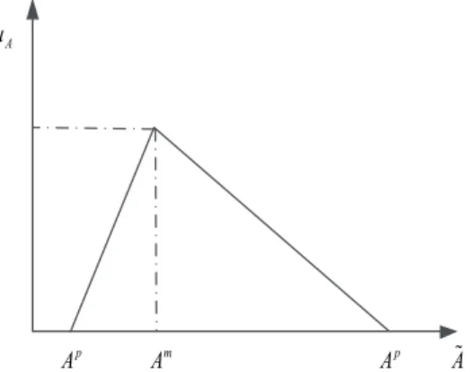
distribution of a fuzzy numberA



A A A_p, _m, _o



, where p

A ,Am, and Ao are the most pessimistic value, the most possible value and the most optimistic value, respectively, which determined by the DMs.

p

A m

A p

A A A



Fig. 1. Triangular possibility distribution of the fuzzy parameter.

The equivalent auxiliary crisp constraints can be demonstrated by:

1

1 , 2 , 3 ,

0 1

(w w w )

n n

p m o

i i i ijk k

i j

d _ d _ d _ x C



 

  



  1 k K (13)

where,

w w

₁

  

₂

w

₃

1

and

w

₁,

w

₂, and

w

₃denote the weights of the most pessimistic, the most possible, and the most optimistic value of the fuzzy demand of customers, respectively. Moreover, β is the minimum acceptable possibility. The optimum values of weights and β usually are determined by the knowledge of the DMs. However, based on the concept of the most likely values proposed by Lai and Hwang (1992), these parameters are considered as:

1 1 3

4 1

w , w w

6 6

   and β = 0.5.

3.2. Step 2: RMCGP

(8)

1

min ( )

n

i i i

i

W d d







(14a)

s.t.

( ) ( )0

k

h X  or k 1, 2, ...,q (14b)

( )

i i i i

f X d d b

  

  i 1, 2,...,n (14c)

, 0

i i

d d  i 1, 2,...,n (14d)

where,h_k(X)is system constraint k,f X_i( )represents goal constraint i,

b

irepresents the aspiration level of

goal i,

d

_iand

d

_iare positive and negative deviations from the target value of goal i, respectively.

( ) if ( ) 0 otherwise

i i i i

i

b f x f x b

d    _

  (15)

( ) if ( ) 0 otherwise

i i i i

i

f x b f x b

d    _

  (16)

The standard GP method emphasizes to find the best solution that is near to the aspiration level of objectives, and also attempts to minimize deviations from aspiration levels. However, in reality, considering exactly one level for aspiration level is not useful and DMs like to determine cautious primary aspiration levels based on available information. The multi-choice goal programming helps to the DMs in making decisions by preventing understatement of the decisions. Chang (2007) presented a new method to solve the multi-choice goal programing (MCGP) for multi-objective decision problems by multiple aspiration levels. The MCGP is formulated as follows:

1 2

1

min

( )

...

n

i i i i im

i

W f X

g or g or

g







(17a)

s.t.

( ) (

)0

k

h x

  

or

k 1, 2, ...,q (17b) where,

g

ij(i=1,2,…,n and j=1,2,…,m) is the j-th aspiration level of the i-th goal

g

ij1



g

ij



g

ij1. The

MCGP method can be formulated by:

1

m in ( )

n

i i i

i

W d d







(18a)

s.t.

( ) ( )0

k

h X  or k 1, 2, ...,q (18b)

1

( ) S (B)

m k i i ij ij

j f X d d g



  



i 1, 2,...,n (18c)

,

0

i i

d d

 



i 1, 2,...,n (18d)

S (B )ij Ri(X ) i 1, 2,...,n (18e)

where,

S B

_ij

 

represents a function of binary serial numbers. Chang (2008) presented the revised approach

for MCGP, which named RMCGP to solve the multi-objective decision problems without employing binary variables, used in the MCGP achievement function. The MCGP-achievement can reformulate in two conditions; ‘the more the better’ and ‘the less the better’. The first condition is formulated by:

1

min (

)

(

)

n

i i i i i i

i

W d



d





e



e

















(19a)

(9)

( ) ( ) 0

k

h X  o r  k 1, 2, ...,q (19b)

( )

k i i i

f X dd y i 1, 2,...,n (19c)

.max

y

_i

  

e

_i

e

_i

g

_i i 1, 2,...,n (19d)

.min .max i i i

g

 

y

g

i 1, 2,...,n (19e)

, , , 0

i i i i

d  d  e e  i 1, 2,...,n (19f)

The second condition is formulated by:

1

min (

)

(

)

n

i i i i i i

i

W d



d





e



e

















(20a)

s.t.

( ) ( )0

k

h X  or  k 1, 2, ...,q (20b)

( )

k i i i

f X

 

d



d





y

i 1, 2,...,n (20c)

.min

y

_i

  

e

_i

e

_i

g

_i i 1, 2,...,n (20d)

.min .max i i i

g

 

y

g

i 1, 2,...,n (20e)

,

, ,

0

i i i i

d d e e

   



i 1, 2,...,n (20f)

where,

g

_{i max}_. is the upper bound of the i-th aspiration level,

g

_{i min}_. is the lower bound of the i-th aspiration

level, is the continuous variable with a range of

g

_{i min}_.

 

y

_i

g

_{i max}_. , d_iand di

_{are positive and negative}

deviations from

f X

_i

(

)



y

_i and

w

_iis the weight of the i-th goal. For the first case:

e

i



and

e

i



are positive

and negative deviations from

y

_i



g

_i_.max and



_i is the weight of the sum of deviations of

y

_i



g

_i_.max . In the second case:

e

i



and

e

i



are positive and negative deviations from

y

_i



g

_i_.min and is the weight of

the sum of deviations of

y

_i



g

_i_.min .

Regarding to the explained method in Sections 3.1 and 3.2, the proposed model is presented by:

1 1 1 1 1 1 2 2 2 2 2 2

min W (

d



d



)





(

e



e



) W (



d



d



)





(

e



e



)

(21)

s.t.

Constraints (3)-(8),(11)-(13)

1 1 1 1

Z

  

d



d



y

(22)

1 1 1 1.min

y

  

e



e



g

(23)

1.min 1 1.max

g

 

y

g

(24)

2 2 2 2

Z

  

d



d



y

(25)

2 2 2 2.min

y

  

e



e



g

(26)

2.min 1 2.max

g

 

y

g

(27)

1

,

1

, , ,

1 1 2

,

2

, ,

2 2

0 d d e e d d e e

       



(28)

where,

d

₁is the positive deviation variable of Z1;

d

₁



is the negative deviation variable of Z1;

d

₂



is the

positive deviation variable of Z2;

d

2



is the negative deviation variable of Z2;

e

1



(10)

from

y

₁



g

_1._min ;

e

₁ is the negative deviations from

y

₁



g

_1._min ;

e

₂is the positive deviations from

2 2.min

y



g

;

e

2



is the negative deviations from

y

₂



g

_2._min . The value of

g

_{i min}_. and

g

_{i max}_. can determined below:

1.min

g

: can be determined by Minimizing Z1

1.max

g

: can be determined by Maximizing Z1

2.min

g

: can be determined by Minimizing Z2

2.max

g

: can be determined by Maximizing Z2

The DMs can determine the

g

_{i min}_. and

g

_{i max}_. by considering the solutions of the mentioned sub-problems

and by consulting with experts.

3.3. Simulated annealing

SA is derived from the analogy to annealing in solids and the solving method of combinatorial optimization problems. For the first time, the main idea proposed by Metropolis et al. (1953). For the first time, SA is used to solve the optimization problems by Kirkpatrick (1984). Usually, optimization problems have some local optimal points. Simple optimization algorithms search the local optimum points by selecting a random initial solution and obtaining the neighbor from solutions. Usually, the simple algorithms stopped the searching due to convergence to local optimum points. However, SA prevents to stay in the local optimum point through accepting cost increasing neighbors with some probability. The parameters setting of SA algorithms such as the initial temperature (T0), the number of neighborhoods, and a temperature reduction factor (α) have a significant impact on the performance of SA. In this algorithm to find the optimum solution, in the first step, the initial solution generated randomly and then in the around of the initial solution neighbor is searched. SA has some advantages and disadvantages compared to other meta-heuristics, such as GA and particle swarm solution (PSO). The advantages of this algorithm (e.g., easier implementation, convergence attributes and utilizing hill climbing) make it popular from meta-heuristic algorithms in the recent decade (Subramanian et al., 2013).

3.4. Genetic algorithm

As mentioned in the literature review section, the GA is one of the most popular algorithms used to solve VRPTW problems. This algorithm is a heuristic search algorithm that mimics evolution through natural selection. In this algorithm, the procedure of searching begins with a set of chromosomes mentioned as the initial population. The initial solution can be generated randomly or created by heuristic methods. The new population is created based on the crossover operator and then mutation operator is utilized. The fitness function is used to select the best solution. Finally, a maximum number of generations or other stopping criteria such as a computational time limit can stop the algorithm.

3.4.1. Solution representation

The solution structure for two proposed meta-heuristic algorithms is same. Fig. 2 demonstrates the possible solution of instance consists four vehicles and 10 customers.

(11)

As can be seen from Fig.2, two different routes separated with each other by index 0; each number demonstrates the customer that is served by vehicles. If the number of routes be less than vehicles number, it means to serve the customers, there is no need to use all of the vehicles. The proposed solution structure permits to minimize the number of vehicles used and the required number of vehicles simultaneously.

3.4.2. Best cost-best route crossover (BCBRC)

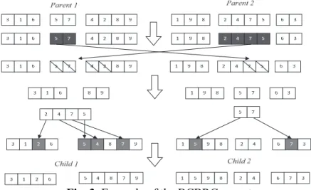
In this paper, the initial solution is generated through an appropriate proposed structure that presented in the previous section. A crossover operator exchanges the information between two chromosomes. In the field of the VRPTW, an appropriate crossover operation should not damage the best solution. Moreover, it should improve the well-known solution to create a better solution. However, some unsuitable crossover operators may create infeasible solutions for VRPTW problems (i.e., classical one-point crossover; due to the excluding or failing of vertices after reproduction) (Ghoseiri & Ghannadpour, 2010). Ombuki et al. (2006) presented a best cost-route crossover (BCRC) to minimize the required number of vehicles and total distance cost by considering the feasibility of constraints. The other version of the BCRC operator proposed by Ombuki-Berman and Hanshar (2009), named best cost-best route crossover (BCBRC). In this operator, the best route is selected by considering the average objective function of nodes. Fig. 3 demonstrates the structure of the BCBRC operator.

3.4.3. Sequence-based mutation (SBM)

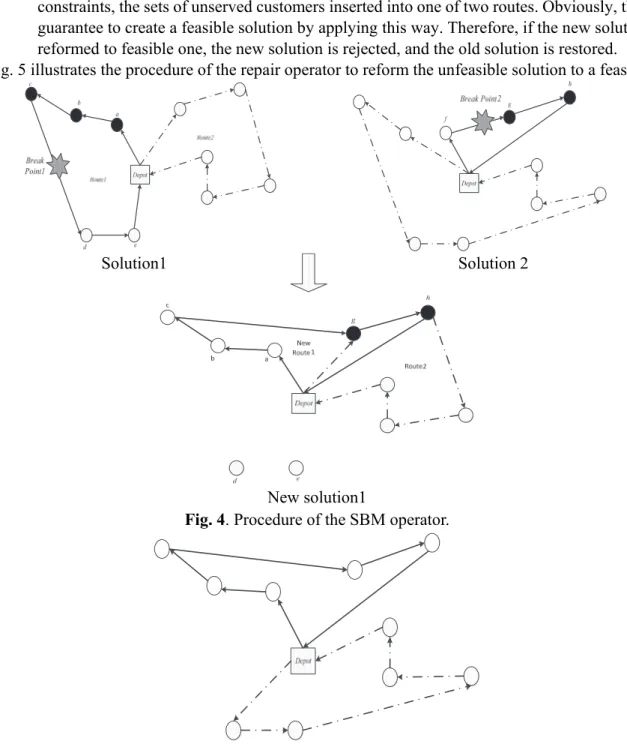
The main aim of the mutation operation is to prepare algorithms to gain local random research ability. The procedure of the proposed SBM operator includes two steps. Two produced solution from the crossover operator is selected. In the first step, from each solution, a link is selected randomly to break a route and then make a change in the routes before and after the break points to make new solutions. Fig. 4 demonstrates the procedure of the SBM operator to create a new solution. As can be inferred from this figure, this operator chooses break point 1 from solution 1 and break point 2 from solution 2, randomly. Then a connection between the route of customers served before the break point 1 and the route of customer serviced after the break point 2 is created. By applying this procedure, the new solution is created. As can be seen from Fig. 4, in the generated solution, a new route is created that namely “New Route1” from removing Route1 and preserving Route2. Likewise, the second new solution can be made by creating a connection between the route of customers served before the break point 2 and the route of customer serviced after the break point 1.

Fig. 3. Example of the BCBRC operator.

(12)

served at the end of the route. Due to some customers are duplicated or removed for servicing, a repair operator is utilized to repair this solution to feasible solution. For instance, in Fig. 4, two customers in new solution 1 are located on the both of the routes (customers g and h), and the customers d and e are not served. The repair operator reforms the unfeasible solution to feasible one in the following ways:

• If a customer located in both of the routes, the customers removed from one of two routes randomly.

• If a customer is removed from routes, then by considering the time window and capacity constraints, the sets of unserved customers inserted into one of two routes. Obviously, there is no guarantee to create a feasible solution by applying this way. Therefore, if the new solution is not reformed to feasible one, the new solution is rejected, and the old solution is restored.

Fig. 5 illustrates the procedure of the repair operator to reform the unfeasible solution to a feasible one.

Solution1 Solution 2

New solution1

Fig. 4. Procedure of the SBM operator.

(13)

4. Computational experiments

The proposed model is validated by solving some test problems. The detail of the parameters’ distribution functions is listed in Table 1. To solve large-sized test problems, SA and GA are used. The performance of proposed meta-heuristic algorithms is compared with each other and LINGO software. Both of SA and GA algorithms are compiled in MATLAB 7.1 on the personal computer including, Intel Core 2 Duo 2.6 GHz processors and 2 GB RAM. In this section, the performance of the proposed SA and GA in terms of solution quality and computational time is evaluated in some randomly generated problems. Each algorithm runs for five times and the best result is reported. The parameter setting of meta-heuristic algorithms have considerable effect on their performance. In this paper, the parameter settings of the proposed meta-heuristics is tuned by the response surface methodology (RSM). The optimum parameter settings of SA and GA algorithms are tabulated in Tables 2 and 3, respectively. The solutions of GA and SA are compared with the optimal solutions obtained from LINGO software in small-sized test problems. Moreover, for large-sized problems that LINGO software cannot reach the optimum solution at the reasonable time. The comparison result between the proposed meta-heuristics in small-sized problems is reported in Table 4. In small-sized problems, a gap between SA and GA with LINGO software is reported through the percentage of relative gap measure that calculated based on [100 × (GLINGO− GMeta)/GMeta], where GLINGO and GMeta are the objective function value (Eq. (21)) of LINGO software and meta-heuristic algorithm, respectively. Moreover, for large-sized problems, the gap between GA and SA is presented based on [100 × (Gbest-Meta − GMeta)/GMeta] in which, GMeta is the objective function of the obtained solution over meta-heuristic methods and Gbest-Meta is the objective function value of meta-heuristic methods that have better performance. Each meta-heuristic method runs for five times and the average gap is reported in Table 5. As can be inferred from Table 5, SA outperforms GA in terms of the solution quality in the all of the test problems. Based on the RMCGP method, the solution procedure of meta-heuristics

algorithms includes two steps. First, the values of

g

1.min,

g

1.max,

g

2.min, and

g

2.maxare obtained in each replication for five times and the best one is selected. Then, based on the obtained results from the previous step, the value of the objective function (Eq. (21)) is calculated. The required computational times for the proposed meta-heuristics are reported in Table 5. The required computational time increased sharply as the test problem size becomes larger. The results demonstrate that GA and SA can obtain a near-optimum solution in a reasonable time especially in large-sized problems. As can be seen from Table 5, the required computational time of GA is more than SA.This difference is derived from the fact that GA has some additional mechanisms (e.g., selection mechanism and crossover), which is time consuming. Moreover, a paired t-test was carried out to compare the runtime of SA and GA. The result of the t-test is illustrated in Table 6. As can be inferred from Table 6, the significant difference is not shown from the result of the t-test.

Table 1

Sources of random generation of the parameters.

Parameter Value Parameter Value

ij

t

U(0.5,5.25)

i

a

U(3.5,6)

k

C _U(95,115)

i

b

U(5,9.5)

i

d



U(11,25) F 2000

i

S

U(0.2,1)

(14)

Table 2

Parameter settings of SA.

Parameter Initial temperature Temperature reduction rate No. of neighborhood

value 100 0.97 40

Table 3

Parameter settings of GA.

Parameter Population size Crossover rate Mutation rate

value 250 0.7 0.4

Table 4

Average relative gaps and CPU time for small-sized test problems.

Data set

SA GA

n K Replications Gap (%) Time(s) Replications Gap (%) Time(s)

1 2 3 4 5 1 2 3 4 5

1 8 3 .00 .00 .00 .00 .00 .000 32 .00 .00 .00 .00 .00 .000 39 2 10 3 .00 .00 .00 .00 .00 .000 37 .00 .01 .00 .00 .00 .002 42 3 12 4 .00 .00 .01 .00 .00 .002 42 .00 .01 .01 .00 .00 .004 51 4 14 4 .01 .00 .00 .01 .00 .004 48 .01 .02 .01 .01 .01 .012 53 5 20 4 .01 .00 .02 .01 .02 .012 53 .02 .02 .03 .01 .02 .02 64 6 25 5 .01 .02 .01 .02 .01 .014 59 .04 .03 .05 .02 .02 .032 71 7 30 5 .02 .03 .03 .04 .02 .028 62 .06 .05 .06 .03 .04 .048 75

Table 5

Average relative gaps and CPU Time for large-sized problems.

Data set SA GA

n K Time(s) Gap (%) Time(s)

8 40 6 73 3.12 89

9 45 6 81 3.26 101

10 50 7 92 3.82 109

11 60 9 106 4.06 123

12 70 10 124 4.59 142

13 80 12 146 5.17 175

14 85 13 165 5.32 204

15 90 14 193 6.24 230

16 100 16 237 7.03 284

17 120 18 264 7.82 328

18 140 20 302 9.24 376

19 145 22 357 10.36 441

20 160 25 391 11.59 586

Table 6

Result of the t-test for SA and GA computational time.

Meta-heuristics SA GA

Mean 143.2 179.15

Variance 12453.95789 23131.18684

Observations 20 20

Hypothesized Mean Difference 0

df 35

t Stat -0.852274558

P(T<=t) one-tail 0.199928106

t Critical one-tail 1.689572458

P(T<=t) two-tail 0.399856213

(15)

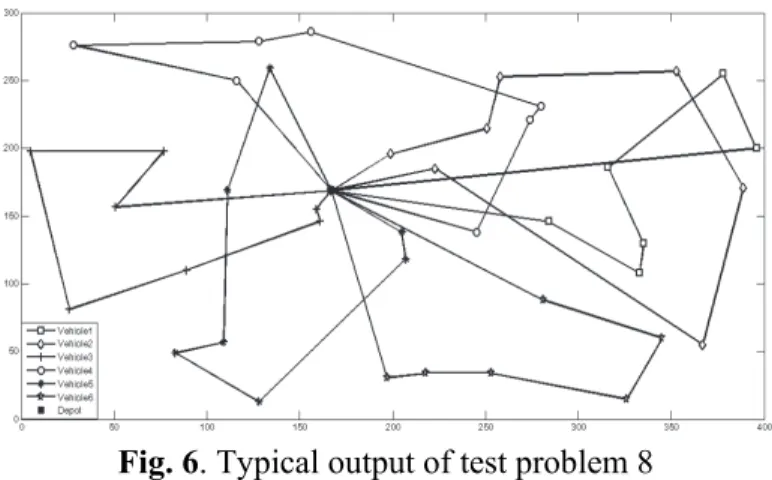
Fig. 6. Typical output of test problem 8

Fig. 6 shows a typical output of test problem 8. In order to determine the effect of the fixed cost of vehicles on the second objective function, the sensitivity analysis is carried out. This experiment is carried out for test problem 7 and all trends can be generalized for other test problems. Fig. 7 demonstrates the sensitivity of the second objective function upon the fixed cost of vehicles increase, in which the second objective function is getting constant or worse regarding by increasing the constant cost of vehicles.

Fig. 7. Impact of increasing the cost of vehicles on the second objective function.

As can be inferred from Fig. 7, the value of the second objective function will be increased by increasing the constant cost of vehicles; however, if the fixed cost of vehicles cost is increased from 300 to 1200 percent, the value of the second objective function remains constant.

4.1. Case study

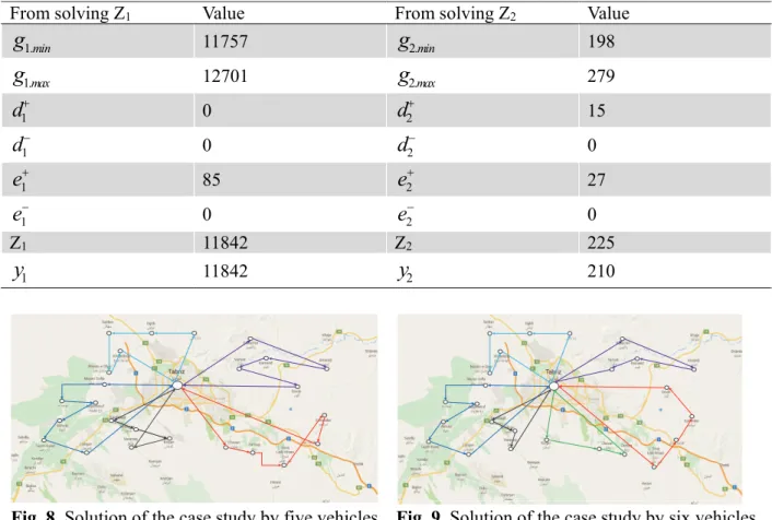
In this section, a real case of goods transportation is studied to validate the performance of the proposed model. The case study is carried out for an international transportation company in Iran. Tranome Tabriz Company (TTC) founded in 1985. This company transports different type of products to all parts of Iran and some Iran’s neighbor countries (e.g., Azerbaijan, Turkey, and Iraq). This company has contracted with the Mohandesan Company (MC) for transporting gas capsule to 25 cities by five available vehicles. The required information gathered from both of the companies. As mentioned in the previous sections, according to a dynamic nature of the environment, the customers’ demand is considered as a fuzzy parameter. The proposed model for TTC is solved in LINGO software. To solve the proposed model, in the first step, the proposed model is converted to an equivalent crisp model. Then, the RMCGP method is used. Table 7 demonstrates the results. As can be seen from Table 7, since the positive and negative deviations of the first goal are zero, the first goal is fully satisfied. However, in the second goal, since the

300 350 400 450 500 550

0 200 400 600 800 1000 1200

The v

alue of second object

ive

funct

ion

(16)

positive deviation is bigger than zero, the second goal has positive deviation. The solution does not satisfy the aspiration level 198 y₂279 and achieves 93.33% of the second goal. Fig. 8 demonstrates the

solution of the case study, in which 25 cities have serviced by five vehicles.

Table 7

Result of the sub-problems by five vehicles

From solving Z1 Value From solving Z2 Value

1.min

g

11757

g

_2._min 198

1.max

g

12701

g

_2._max 279

1

d

 0

d

₂ 15

1

d

 0

d

₂ 0

1

e

 85

e

₂ 27

1

e

 0

e

₂ 0

Z1 11842 Z2 225

1

y

11842

y

₂ 210

Fig. 8. Solution of the case study by five vehicles Fig. 9. Solution of the case study by six vehicles

If the DMs decided to increase the number of the available vehicles from five to six vehicles, the proposed model is resolved. Table 8 demonstrates the result of the problem by considering the six available vehicles.

Table 8

Result of the sub-problems by six vehicles

From solving Z1 Value From solving Z2 Value

1.min

g

11175 g2 .m in 181

1.max

g

13648

g

_2._max 264

1

d

 129

d

₂ 0

1

d 0 d2



0

1

e

 1668

e

₂ 22

1

e

 0

e

₂ 0

Z1 12972 Z2 203

1

(17)

As can be seen from Table 8, positive and negative deviations of the second goal are zero; therefore, the second goal is satisfied fully. However, in the first goal, since the positive deviation is bigger than zero, the first goal has a positive deviation. The solution does not satisfy the aspiration level 11175 y₁13648

and achieves 99% of the first goal. Fig. 9 demonstrates the optimum vehicle routing problem by six available vehicles. As a sensitivity analysis by according to Table 9, it can be comprehended that the value of each objective function increased by increasing the value of Wi corresponding objective function. Therefore, the DMs can adjust the value of objective functions by changing the corresponding Wi. Moreover, the Pareto frontier of the problems is illustrated in Figs. (10-11). As can be inferred from these figures, due to the both of objective functions are minimized, thus the Pareto frontiers for the problem is concave.

Table 9

Result of a sensitivity analysis.

Number of vehicles W1 W2 Z1 Z2

0.8 0.2 11842 225

0.7 0.3 12026 210

5 0.6 0.4 12125 191

0.5 0.5 12265 172

0.4 0.6 12365 160

0.3 0.7 12456 142

0.8 0.2 12843 203

0.7 0.3 12965 184

6 0.6 0.4 13056 162

0.5 0.5 13187 146

0.4 0.6 13263 132

0.3 0.7 13326 127

Fig. 10. Pareto frontier of the problem by five vehicles.

Fig. 11. Pareto frontier of the problem by six vehicles.

100 120 140 160 180 200 220 240

11800 11900 12000 12100 12200 12300 12400 12500

O

b

je

ctiv

e func

ti

on 2

Objective function 1

100 120 140 160 180 200 220

12800 12900 13000 13100 13200 13300 13400

Obj

ecti

v

e fun

cti

on

2

(18)

5. Conclusion

In this paper, a bi-objective possibilistic programming model was developed to formulate the VRPTW by considering the customers’ satisfaction. In the proposed mathematical problem, the first objective function was to minimize the sum of a fixed cost related to the number of vehicles and travel distance, and the second objective function considered the customers’ satisfaction by minimizing the gap time between the arrival time and ready time by considering the customers’ priority. In this paper, for solving the proposed problem, two steps were considered; in the first step, the possibilistic proposed model was converted into an equivalent auxiliary crisp model and in the second step, an RMCGP method was employed to attain an approved adjustment solution. The proposed model provides useful awareness to help the DMs in identifying effective parameters and creates an optimal decision closer to reality. The proposed model provides a suitable way to solve bi-objectives decision-making problems, which includes multi-choice of aspiration levels. The customers’ demand was considered as fuzzy numbers. The proposed model was validated by LINGO software. In order to solve the model in large-sized problems, two meta-heuristic algorithms (i.e., simulated annealing (SA) and genetic algorithm (GA)) is used. The results demonstrated that SA outperforms GA in both objective function values and computational times. Finally, to demonstrate the validation of the proposed model, an industrial case study related to the TTC was investigated.

References

Afshar-Bakeshloo, M, Mehrabi, A, Safari, H, Maleki, M, & Jolai, F. (2016). A green vehicle routing problem with customer satisfaction criteria. Journal of Industrial Engineering International, 12(4), 529-544.

Aouni, B., Martel, J. M., & Hassaine, A. (2009). Fuzzy goal programming model: an overview of the current state‐of‐the art. Journal of Multi‐Criteria Decision Analysis, 16(5‐6), 149-161.

Archetti, C., Speranza, M. G., & Vigo, D. (2014). Vehicle routing problems with profits. Vehicle Routing: Problems, Methods, and Applications, 18, 273.

Barkaoui, M., Berger, J., & Boukhtouta, A. (2015). Customer satisfaction in dynamic vehicle routing problem with time windows. Applied Soft Computing, 35, 423-432.

Belhaiza, S., Hansen, P., & Laporte, G. (2014). A hybrid variable neighborhood tabu search heuristic for the vehicle routing problem with multiple time windows. Computers & Operations Research, 52, 269-281.

Calvete, H. I., Galé, C., Oliveros, M. J., & Sánchez-Valverde, B. (2007). A goal programming approach to vehicle routing problems with soft time windows. European Journal of Operational Research, 177(3), 1720-1733.

Castro-Gutierrez, J., Landa-Silva, D., & Pérez, J. M. (2011, October). Nature of real-world multi-objective vehicle routing with evolutionary algorithms. In Systems, Man, and Cybernetics (SMC), 2011 IEEE International Conference on (pp. 257-264). IEEE.

Chang, C. T. (2007). Multi-choice goal programming. Omega, 35(4), 389-396.

Chang, C. T. (2008). Revised multi-choice goal programming. Applied Mathematical Modelling, 32(12), 2587-2595.

Charnes, A., & Cooper, W. W. (1957). Management models and industrial applications of linear programming. Management Science, 4(1), 38-91.

da Silva, A. F., Marins, F. A. S., & Montevechi, J. A. B. (2013). Multi-choice mixed integer goal programming optimization for real problems in a sugar and ethanol milling company. Applied Mathematical Modelling, 37(9), 6146-6162.

Dantzig, G. B., & Ramser, J. H. (1959). The truck dispatching problem. Management science, 6(1), 80-91.

(19)

Dubois, D., & Perny, P. (2016). A Review of Fuzzy Sets in Decision Sciences: Achievements, Limitations and Perspectives. In Multiple Criteria Decision Analysis (pp. 637-691). Springer New York.

Eksioglu, B., Vural, A. V., & Reisman, A. (2009). The vehicle routing problem: A taxonomic review. Computers & Industrial Engineering, 57(4), 1472-1483.

Forslund, H., & Jonsson, P. (2010). Integrating the performance management process of on-time delivery with suppliers. International Journal of Logistics: Research and Applications, 13(3), 225-241. Gehring, H., & Homberger, J. (2002). Parallelization of a two-phase metaheuristic for routing problems

with time windows. Journal of heuristics, 8(3), 251-276.

Ghannadpour, S. F., Noori, S., & Tavakkoli-Moghaddam, R. (2014). A multi-objective vehicle routing and scheduling problem with uncertainty in customers’ request and priority. Journal of Combinatorial Optimization, 28(2), 414-446.

Ghoseiri, K., & Ghannadpour, S. F. (2010). Multi-objective vehicle routing problem with time windows using goal programming and genetic algorithm. Applied Soft Computing, 10(4), 1096-1107.

Goncalves, G., Hsu, T., & Xu, J. (2009). Vehicle routing problem with time windows and fuzzy demands: an approach based on the possibility theory. International Journal of Advanced Operations Management, 1(4), 312-330.

Hashimoto, H., Ibaraki, T., Imahori, S., & Yagiura, M. (2006). The vehicle routing problem with flexible time windows and traveling times. Discrete Applied Mathematics, 154(16), 2271-2290.

HO, C. J. (1989). Evaluating the impact of operating environments on MRP system nervousness. The International Journal of Production Research, 27(7), 1115-1135.

Hong, S. C., & Park, Y. B. (1999). A heuristic for bi-objective vehicle routing with time window constraints. International Journal of Production Economics, 62(3), 249-258.

Huang, M., & Hu, X. (2012). Large scale vehicle routing problem: An overview of algorithms and an intelligent procedure. Int. J. Innov. Comput. Inf. Control, 8, 5809-5819.

Jiménez, M., Arenas, M., Bilbao, A., & Rodr_ı, M. V. (2007). Linear programming with fuzzy parameters: an interactive method resolution. European Journal of Operational Research, 177(3), 1599-1609. Jones, D. F., Mirrazavi, S. K., & Tamiz, M. (2002). Multi-objective meta-heuristics: An overview of the

current state-of-the-art. European journal of operational research, 137(1), 1-9.

Jones, D., & Tamiz, M. (2016). A review of goal programming. In Multiple Criteria Decision Analysis (pp. 903-926). Springer New York.

Kirkpatrick, S. (1984). Optimization by simulated annealing: Quantitative studies. Journal of statistical physics, 34(5-6), 975-986.

Lai, K. K., Liu, B., & Peng, J. (2003). Vehicle routing problem with fuzzy travel times and its genetic algorithm. Technical Report.

Lai, Y. J., & Hwang, C. L. (1992). A new approach to some possibilistic linear programming problems. Fuzzy sets and systems, 49(2), 121-133.

Lee, C., Lee, K., & Park, S. (2012). Robust vehicle routing problem with deadlines and travel time/demand uncertainty. Journal of the Operational Research Society, 63(9), 1294-1306.

Liao, C. N., & Kao, H. P. (2010). Supplier selection model using Taguchi loss function, analytical hierarchy process and multi-choice goal programming. Computers & Industrial Engineering, 58(4), 571-577.

Melián-Batista, B., De Santiago, A., AngelBello, F., & Alvarez, A. (2014). A bi-objective vehicle routing problem with time windows: A real case in Tenerife. Applied Soft Computing, 17, 140-152.

Metropolis, N., Rosenbluth, A. W., Rosenbluth, M. N., Teller, A. H., & Teller, E. (1953). Equation of state calculations by fast computing machines. The journal of chemical physics, 21(6), 1087-1092. Moghadam, B., & Seyedhosseini, S. (2010). A particle swarm approach to solve vehicle routing problem

with uncertain demand: A drug distribution case study. International Journal of Industrial Engineering Computations, 1(1), 55-64.

(20)

Ombuki-Berman, B., & Hanshar, F. T. (2009). Using genetic algorithms for multi-depot vehicle routing. In Bio-inspired algorithms for the vehicle routing problem (pp. 77-99). Springer Berlin Heidelberg. Ombuki, B., Ross, B. J., & Hanshar, F. (2006). Multi-objective genetic algorithms for vehicle routing

problem with time windows. Applied Intelligence, 24(1), 17-30.

Pillac, V., Gendreau, M., Guéret, C., & Medaglia, A. L. (2013). A review of dynamic vehicle routing problems. European Journal of Operational Research, 225(1), 1-11.

Pishvaee, M. S., & Razmi, J. (2012). Environmental supply chain network design using multi-objective fuzzy mathematical programming. Applied Mathematical Modelling, 36(8), 3433-3446.

Rath, S., Gendreau, M., & Gutjahr, W. J. (2015). Bi‐objective stochastic programming models for determining depot locations in disaster relief operations. International Transactions in Operational Research.

Rincon-Garcia, N., Waterson, B., & Cherrett, T. (2017). A hybrid metaheuristic for the time-dependent vehicle routing problem with hard time windows. International Journal of Industrial Engineering Computations, 8(1), 141-160.

Chávez, J., Escobar, J & Echeverri, M. (2016). A multi-objective Pareto ant colony algorithm for the Multi-Depot Vehicle Routing problem with Backhauls.International Journal of Industrial Engineering Computations , 7(1), 35-48.

Sivaramkumar, V., Thansekhar, M. R., Saravanan, R., & Amali, S. M. J. (2015). Multi-objective vehicle routing problem with time windows: Improving customer satisfaction by considering gap time. Proceedings of the Institution of Mechanical Engineers, Part B: Journal of Engineering Manufacture, 0954405415586608.

Subramanian, P., Ramkumar, N., Narendran, T. T., & Ganesh, K. (2013). PRISM: PRIority based SiMulated annealing for a closed loop supply chain network design problem. Applied Soft Computing, 13(2), 1121-1135.

Taş, D., Dellaert, N., Van Woensel, T., & De Kok, T. (2013). Vehicle routing problem with stochastic travel times including soft time windows and service costs. Computers & Operations Research, 40(1), 214-224.

Torabi, S. A., & Hassini, E. (2008). An interactive possibilistic programming approach for multiple objective supply chain master planning. Fuzzy Sets and Systems, 159(2), 193-214.

Zheng, Y., & Liu, B. (2006). Fuzzy vehicle routing model with credibility measure and its hybrid intelligent algorithm. Applied mathematics and computation, 176(2), 673-683.

Zografos, K. G., & Androutsopoulos, K. N. (2004). A heuristic algorithm for solving hazardous materials distribution problems. European Journal of Operational Research, 152(2), 507-519.