Nº 493
ISSN 0104-8910
Real exchange rate misalignments
Maria Cristina T. Terra
Real Exchange Rate Misalignments
Maria Cristina T. Terra
¤Frederico Estrella Carneiro Valladares
yAugust 18, 2003
Abstract
This paper characterizes episodes of real appreciations and deprecia-tions for a sample of 85 countries, approximately from 1960 to 1998. First, the equilibrium real exchange rate series are constructed for each country using Goldfajn and Valdes (1999) methodology (cointegration with fun-damentals). Then, departures from equilibrium real exchange rate (mis-alignments) are obtained, and a Markov Switching Model is used to char-acterize the misalignments series as stochastic autoregressive processes governed by two states representing di¤erent means. Three are the main results we …nd: …rst, no evidence of di¤erent regimes for misalignment is found in some countries, second, some countries present one regime of no misalignment (tranquility) and the other regime with misalignment (cri-sis), and, third, for those countries with two misalignment regimes, the lower mean misalignment regime (appreciated) have higher persistence that the higher mean one (depreciated).
1
Introduction
In the aftermath of Bretton Woods collapse and the advent of ‡exible exchange rates, many economic models relying on PPP as an equilibrium condition, hav-ing it behav-ing derived as an outcome or a possible violation, could be easily found. Whenever PPP is admitted to fail, the existence of real exchange rate (RER) misalignments is being implicitly assumed, that is, departures from an equilib-rium RER value occur.
In fact, RER misalignments can be found in the core of many of the most studied open economy macroeconomics and international …nance issues. Dorn-busch (1976), for instance, shows that di¤erential speeds of adjustments between commodity and asset markets produce, in response to nominal shocks, short-run deviations from PPP. In the same framework, real shocks can produce a change in the long run equilibrium RER. Calvo and Rodriguez (1977) and Mussa (1982) are also examples of this class of models.
¤I thank Pronex and CNPq for …nancial support. E-mail: [email protected]
This question becomes substantially relevant when the role and possible e¤ects of RER movements over economic and social outcomes are taken into ac-count. Let RER be the relative cost between a common basket of international and domestic goods, measured in the same numeraire. Hence, it can be under-stood as thetrue indicator of the incentives to the economic agents regarding the production and consumption decisions between domestic and international goods. Therefore, RER movements - under a few theoretical conditions - can a¤ect both national savings and domestic absorption with real economic e¤ects. In addition, this problem has also been addressed in another perspective. Persistent exchange rate misalignments can generate severe macroeconomic dis-equilibria usually leading to costly external imbalances corrections. Both the-oretical and empirical literatures on speculative attacks, for example, attach a signi…cant position to RER appreciations. Following Krugman (1979) semi-nal work, …rst generation speculative attacks models modi…ed versions allowing PPP deviations were developed. This advance leads to RER appreciation as an empirical regularity that should be seen in the run-up of such events. Evidences of RER appreciations as an early warning indicator of possible currency crisis episodes have been recently widely documented.1
A broad range of studies has been developed in the recent decades in order to discuss whether and how purchasing power parity (PPP) hypothesis is a reasonable assumption. As stated in Rogo¤ (1996), few studies suppose that PPP holds in the short-run (continuously). In fact, the literature has been concentrated on whether there exists reversion of real exchange rates towards a long-run mean. The underlying idea on this approach is to investigate if real exchange rate misalignments (appreciations and depreciations) around a long-run equilibrium value vanish.
Goldfajn and Valdes (1999) go beyond this question and assume that RER, as a rule, reverts to a time-varying long run equilibrium value. The authors are especially concerned about how (instead of whether) real appreciations revert to the equilibrium level. Two main questions are addressed in their paper. The …rst is related to the construction of an acceptable methodology in order to characterize movements on observed RER as deviations from an equilibrium value. The second issue discussed is the assessment of how these appreciations episodes end, that is, which component of the RER (nominal exchange rate or price level di¤erential), after a maximum degree of overvaluation has been achieved, is the main responsible for the return to the equilibrium value.
Two alternative methods for estimating a suitable empirical proxy for the equilibrium real exchange rate (ERER) are employed in Goldfajn and Valdes (1999): a plain Hodrick-Prescott …lter on observed RER and the estimation of a long run relationship between RER and economic fundamentals using cointegra-tion techniques. An overvaluacointegra-tion series is then constructed involving the ob-served RER and the predicted value for both mentioned methodologies. When the overvaluation index is above a certain threshold, the associated period is
1See, for example, Eichengreen, Rose and Wyplosz (1995), Kaminsky, Lizondo and
classi…ed as an appreciation episode. Using a statistical framework, the number and dynamics of appreciations for multiple limits. As expected, they found that the number of appreciations is a negative function of the appreciation thresh-old. An important drawback of this approach is that the threshold used to identify appreciations is largely arbitrary. Consequently, the methodology used to classify observations may be quitead hoc.2
This paper is mainly focused on the characterization of both real appreci-ations and depreciappreci-ations episodes trying to set up a methodology that do not depend on individual discretion on the classi…cation of whether a departure from equilibrium RER is big enough to be considered a meaningful economic episode (real appreciation and depreciation). Firstly, equilibrium RER series are constructed using Goldfajn and Valdes (1999) methodology (cointegration with fundamentals) for a large subset of countries covered in their paper.3
Af-ter the departures from equilibrium RER (misalignments) have been obtained, a Markov Switching Model (MSM) is used to model the misalignments series as stochastic autoregressive processes governed by two states representing di¤erent means. This speci…c econometric characterization allows testing the plausibility of two states without an user de…ned ad-hoc threshold. In theory, each mean can be interpreted as signaling the existence of appreciations or depreciations episodes.
Some important results are found. In …rst place, some countries do not present statistical evidence that di¤erent regimes should be considered for mis-alignments. Second, the misalignments processes characteristics, jointly with the supposed probabilistic structure, favors the detection, in some cases, of states that can be understood as crises and tranquility states, instead of appre-ciation and depreappre-ciation outcomes.
The results obtained also seem to indicate that the threshold issue discussed above is relevant. Alternative regimes are found for some of those countries whose departures from ERER are not large, using Goldfajn and Valdes (1999) - hereafter GV - metric. Hence, an endogenously determined limit for apprecia-tions/depreciations that takes into consideration the series behavior across time seems to be adequate. Finally, evidence of a di¤erent behavior of RER depar-tures under di¤erent regimes is found. Lower mean misalignments are reported as having higher persistence than higher mean misalignments.
In the MSM model, at each point of time, the current state of the underlying series is unknown and statistical inference about the likelihood of being on a speci…c state can be made. Hence, it is also possible to markedly establish starting and ending points for real appreciation and depreciation episodes. A comparison between both methods is made for the whole set of countries and
2The authors implicitly acknowledge this problem on the de…nition of the overvaluation
bound and study, using a statistical framework, the number and dynamics of appreciations for multiple limits. As expected, they found that the number of appreciations is a negative function of the appreciation threshold.
3With the bene…t of additional data, the period covered is extended up to 1998. This
some remarkable di¤erences appear. Maybe, partially in‡uenced by the above mentioned tranquility/crises pattern, both the number and average duration of misalignments episodes are higher than those …gures calculated by GV.
This paper is organized as follows. The next section discusses the estimation of the RER misalignments using the cointegration with fundamentals approach. The third section uses the previous section misalignments estimates as inputs to a two-state Markov Switching Model. The …nal section concludes.
2
Real exchange rate misalignments estimation
An important e¤ort on RER misalignments studies relies on the proper esti-mation of the equilibrium real exchange rate. The empirical de…nition here employed is, to a certain extent, the culmination of a wide debate on PPP deviations. A special strand of the literature, usually interested in predicting nominal and real exchange rates behavior in the long run, assumes that RER series are permanently a¤ected by shocks and adopts the idea that the equilib-rium real exchange rate changes over time. [See, for example, Mark (1995)]. As a consequence, the idea of a long run constant mean level underlying PPP is abandoned. The exchange rate continues to return to a target level although it is not the PPP anymore.4
A natural extension to this approach is to allow equilibrium exchange rate to be a function of other economic factors – hereafter denominated fundamentals – that have an e¤ect on the equilibrium RER and try to derive a long run equilibrium relationship among all these variables. This is precisely one of the practices adopted in Goldfajn and Valdes (1999) and also used in the present work. Hence, most of the work here performed is similar to that present in GV. The method basically consists of estimating a cointegrating relation between observed RER and a chosen set of economic fundamentals. Implicitly, there is the assumption that the RER can be decomposed into a permanent component, that is, a non-stationary I(1) series, and another element that has a stationary behavior. The integrated component represents those changes in the RER that do not vanish over time, namely, changes in the ERER. The I(0) elements are the short-run misalignments that disappear over time.5
4The core inspiration for such change can be attributed to Balassa-Samuelson e¤ects. In
this case, a trend in the equilibrium real exchange rate can be derived from di¤erences of productivity growth rates of tradables and nontradables sectors among di¤erent countries. The key idea is that in a country in which tradables sector productivity, relatively to nontradables, grows steadily faster than its partners, the price of nontradable goods has a tendency to increase, thus entailing a long-run real exchange rate appreciation. Two hypothesis are crucial to this result: free capital mobility between both countries and sectors and lack of labor mobility between countries, even though it is allowed to move from a sector to another. [See Obstfeld and Rogo¤ (1996)]
5The …rst step is to test for the existence of cointegration among the series. Then an
uni-variate estimation method is performed to estimate the cointegrating relationship. Di¤erently
from GV, OLS estimation is performed here. The authors reveal that “Stock-Watson approach
Once a cointegrating vector has been found, an equilibrium RER series is constructed applying the cointegrating vector to the fundamental series. At each point of time, an equilibrium value to the RER is reached and the di¤erence between the observed RER and the calculated equilibrium RER is the real exchange rate misalignment. This task was accomplished for a subset of 85 countries - from a total of 93in GV and the data used is described in the following subsection.6
2.1
Data
Following Goldfajn and Valdés (1999), whenever possible – in terms of availabil-ity or reliabilavailabil-ity – WPIs were used to construct the RER series. In other cases, they are replaced with CPIs as speci…ed in GV. The monthly data required for this task – average monthly nominal exchange rates and price indexes – were mainly obtained from International Financial Statistics- IMF covering a period ranging from January 1960 through December 1998. All series were graphically examined in order to avoid data glitches. As in GV, price indexes missing values for some short periods of time were obtained via interpolation.
Bilateral exchange rates for each country were calculated for those coun-tries encompassing more than 4% of total trade. Subsequently, after a suitable normalization of these series to avoid scale problems (Jan/1990 = 100), a mul-tilateral real exchange rate was obtained for each country, properly weighting the bilateral series by their respective relevance on trade.7
In accordance with GV, four economic fundamentals are used to capture changes in RER attributable to structural rather than transitory factors: terms of trade, openness, government size and international interest rate. The impacts of these fundamentals on RER as well the characteristics of the data used as proxies to these economic factors are shortly addressed below.
Terms of Trade (TOT): The usual simpli…cation that all countries produce the same varieties of tradable goods is not reasonable in practice. In fact, the goods a country exports has a degree of di¤erentiation from those it imports. Obstfeld and Rogo¤ (1996) draw attention to the point that terms of trade – the relative price of exports to imports – are one of the main channels of global transmission of macroeconomic shocks. The outcomes of these relative price changes over RER are associated to adjustments on nontradables prices due to demand shifts. Following Diaz-Alejandro (1982) long-established approach, a negative (permanent) TOT shock – that is, an increase in import prices com-pared to export prices – imparts a nontradables price decrease caused by the fall in real income. A real depreciation is attained in equilibrium.8 The main
source for TOT data used is the World Development Report from World Bank,
of reasoning but we make a case for OLS estimation, as it is also a consistent estimator.
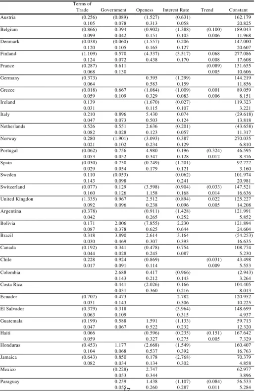
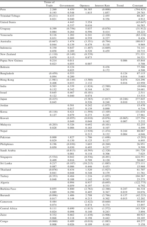
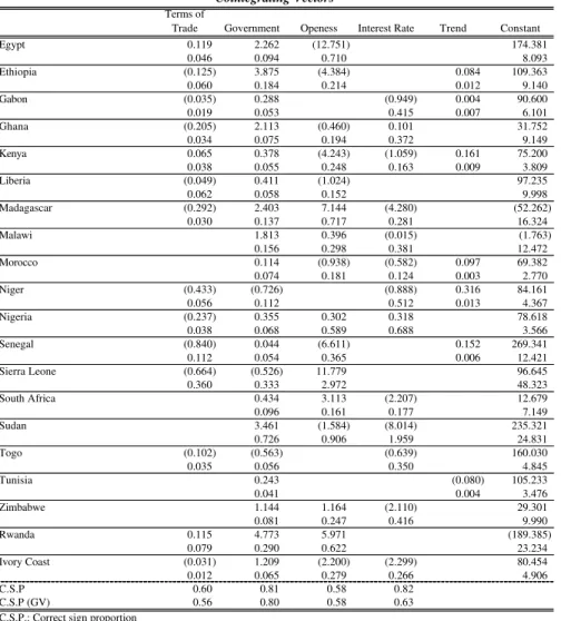
6Due to space restrictions, Table 1 in Appendix I presents a sample of the cointegrating
relationships estimated for the whole set of 85 countries covered in this paper.
7We use the same weights as GV. The resulting multilateral RER was considered available
for a speci…c month only when all bilateral series were available for that month.
8We assume this line of reasoning in the subsequent analyses even though an opposite
completed with IFS exports and imports prices when possible. As these data are available in annual basis, the same course of action of GV to convert it to monthly data was employed, that is, yearly data was linearly interpolated using June as the basis month.9
Openness (OPEN): This variable is, to some extent, a measure that indicates the degree to which the country is a¤ected by the international environment – how much it is connected to the rest of the world. Here, it is proxied by the sum of exports and imports over GDP. A real depreciation is observed in equilibrium when openness level is higher. The reason is quite simple: a trade liberalization reduces domestic prices of tradables causing a demand shift from nontraded goods towards those that are traded. Under some fairly reasonable cross price elasticities assumptions, nontradables prices must fall and a real depreciation is reached in equilibrium.
Size of Government (GOV): A permanent change in the size of government a¤ects RER whenever it triggers demand swings from tradables to nontrad-ables. Countries where government spending is likely to fall more heavily on nontradable goods relative to private spending should experience equilibrium RER appreciations following an increase in the size of government. 10
Goldfajn and Valdés (1999) uses, as proxies for the last two fundamentals, the statistics provided by Penn World Tables (PWT 5) identi…ed as Openness and Real Government share of GDP for the period between 1960-1992. From 1992 to 1994, World Bank data is used. We take bene…t of a new set of data covering a period up to 1998 (PWT 6.0). Besides the time extension, another advantage follows: the use of two sources of data is avoided.
The series from both data sets were compared for the overlapping periods and remarkable divergences in some cases were found related to level as well as dynamics. The disparities on the series levels are related to di¤erent rela-tive price systems among aggregates as a consequence of di¤erent starting points (PWT 5.6 data is measured in 1985 prices and PWT 6.0 has 1996 as basis). The constant price share of government spending, for a particular year is di¤erent when valued in 1996 international dollars than when valued in 1985 interna-tional dollars.11 This di¤erence, however, does not in‡uence the estimation of
the cointegrating vector in order to establish the long-run relationship between RER and fundamentals. The discrepancies observed in the dynamics of the fun-damental, however, do have consequences on the equilibrium RER assessment.
9The monthly government consumption and the degree of openness were also obtained
using this technique.
1 0There is some controversy in this topic, however. Rogo¤ (1992) argues that as long as
capital and labor are fully mobile cross sectors, this e¤ect might be transitory. Essentially, supply factors in place of demand factors should exhibit a long run e¤ect on RER.
11PWT data is constructed departing from International Comparison Program (ICP)
It is important to highlight that these changes are not connected to substantial methodological shifts but rather to growth rates adjustments for a subset of countries. National accounts growth rates for a number of countries have been updated, thus altering these indicators dynamics.12
International Interest Rate (TBAA3M): A gap between domestic and inter-national interest rates has opposite outcomes on RER when short and long run perspectives are considered. Lower international interest rates strengthen capi-tal ‡ows and thus generate an appreciation tendency in small open economies. On the other hand, in the long-run, as it can be associated with a smaller net as-sets accumulation, it might be consistent with a equilibrium RER depreciation. The US 3-Month Treasury Bill is used to capture this e¤ects.
Summarizing the arguments discussed above, the following relationships with equilibrium RER are expected to hold in the long-run:
@ERER @T OT <0;
@ERER @OP EN >0;
@ERER @GOV <0;
@ERER
@T BAA3M <0 (1)
Table 1 in the Appendix presents the estimated cointegrating vectors.13
3
Misalignments and MSM
The preliminary assessment of the misalignments previously computed indicates that it can be characterized as stochastic processes with substantial degree of persistence. In fact, for many countries studied, misalignments seem to be up to long swings, that is, to move in one direction for long periods of time. Additionally, these movements are frequently succeeded by sudden shifts on its values towards the opposite direction. This stylized fact is in harmony with GV inertia of RER when the latter is outside its equilibrium path. Besides, it seems to be coherent with the low probability of smooth returns of appreciation episodes.
These long swings followed by sudden reversals suggest the Markov Switching Model as a suitable description for such class of processes. The MSM deals with situations in which discrete shifts in regime are possible, that is, the existence of “episodes across which the dynamic behavior of the series is markedly di¤erent.” (Hamilton, 1989, p.358). Additionally, no previous knowledge of the state of the stochastic process is required. In fact, this becomes a probabilistic inference problem in which every observation is assigned a probability of being originated from a speci…c regime.
Many empirical questions are up to be addressed with this model. Hamil-ton (1989) originally makes use of this framework to estimate the likelihood of
12Burundi, Morocco and Syrian Arab Republic are some of the countries where this
phenom-ena is seen on government spending. Openness series are less prone to signi…cant divergences but they can be observed for Bolivia, Algeria and Sierra Leone for example. We do thank Bettina Aten for her invaluable informations regarding the series construction procedures.
13All tables in the Appendix presents the results for a subset of the countries in this study,
two regimes for US GNP growth. The paper illustrates that a high probabil-ity of being in a low growth rate regime, as a general rule, is associated with those periods characterized as recessions by the National Bureau of Economic Research. Martinez-Peria (2002), particularly interested on exchange market pressure, models the mechanics of swings from tranquil to speculative attack regimes (and vice-versa). Engel and Hamilton (1990) develops a MSM model in order to assess shifts on the dollar nominal exchange rate and shows that it has a better predictive performance than a simple random walk model. Fi-nally, Bonomo and Terra (1999), focusing on Brazilian exchange rate political economy, makes use of an extended version of Hamilton’s model to obtain, in addition to whether real exchange rate misalignments have di¤erent regimes, the political factors that may in‡uence the shifts from one regime to another. Engel and Hakkio (1996) and Kaminsky (1993) are also examples of the use of MSM to exchange rates.
Here, the focus is on whether distinct regimes for misalignments exist. At …rst, we presume that overvalued and undervalued states will arise. The estima-tion may either con…rm the existence of two misalignment states, or it may show that only one regime is the best description for the misalignment. As already mentioned, a straightforward advantage of this model is that is endogenously determines the existence of alternative regimes. This is particularly relevant if we take into consideration that the level of misalignment that may have e¤ect on economic outcomes can be quite di¤erent on a country basis. More clearly, depending on alternative social and economic structures – such as institutions or exchange rate arrangements, for example – the same level of departure from RER may or may not be considered a relevant economic episode (a real appre-ciation or depreappre-ciation). Indeed, it is reasonable to suspect that appreappre-ciations and depreciations may have also di¤erent cuto¤s. These questions are examined here.
The MSM model as well as its empirical implementation to the RER mis-alignments is presented in the next subsection. Some comparisons of the results obtained with those available from GV then follow.
3.1
Markov Switching Model implementation
The RER misalignment is modeled as following an auto-regressive stochastic process ruled by alternative states which have di¤erent means and variances. A Markov Switching Model is used to characterize such process, and it may be described by the following equation:
mt¡¹(st) =Á(mt¡1¡¹(st¡1)) +¾(st)»t (2)
wheremtis the RER misalignment,f»tgis a sequence of i.i.d. N(0;1)random
variables, andstis an unobserved variable governing both the mean term¹and the variance ¾. Basically, the stochastic process is an autoregressive process that ‡uctuates around two di¤erent means. The variablest is usually referred
is at each moment. Hence, the dynamics of the stochastic process is de…ned by the interaction of the autoregressive coe¢cientÁ, the gaussian innovations »t,
andst.
The variable st is modeled as a discrete-valued stochastic process that can assume distinct values and we will admit two states as possible, henceforth la-beled states one (depreciated) and two (appreciated). Consequently, the actual misalignment series may have observations that can come from alternative sto-chastic processes with two di¤erent means and possibly also di¤erent variances. As usual,stis modeled as a …rst-order Markov process in which the current state depends only on the state in which the stochastic variable was in the immediate preceding period.
LetfstgTt=1 be the sample path of the Markov process described above. A
transition probabilities matrix can be de…ned by:
P =
·
p11 1¡p22 1¡p11 p22
¸
(3)
wherepiiis the probability that the economy will remain in stateinext period. We de…nepii= exp(¯i)
1+exp(¯i). The transition probabilities, written as logistic
func-tions from parameters¯i, are time invariant. Our main focus in this paper is
on the probability of being, in a given point of time, in a speci…c regime (with a higher or lower mean).
The model is estimated using maximum likelihood. For this reason, some hypothesis might be made concerning the conditional distribution of the mis-alignments in such a way that a likelihood function can be built. Mismis-alignments sample pathfmtgTt=1 are assumed to be a stochastic process characterized as a
gaussian i.i.d. mixture that depends on the unobserved state variable sample path. Therefore, the density ofmt conditional onsthas a normal distribution:
f(mt=st=i;®i) = p1
2¼¾iexp
(
[(mt¡¹i)¡Á(mt¡1¡¹i)] 2
2¾2 i
)
(4)
for®i= (¹1; ¾i; Á)a vector of population parameters and i = 1,2.14
The estimation problem reduces to …nding a set of parameters that maxi-mizes the log likelihood function subject to the usual constraints on transition probabilities. Once a set of parameter estimates has been found, a sequence of estimates for the (constant) transition probabilities is also available. Such estimates can be used to form …ltered probabilities which assess the likelihood of the states at each point of time.15
14It is important to remember that normality assumption regards the conditional rather the
unconditional distribution of misalignments. The actual misalignments series are supposed gaussian mixtures and may have completely di¤erent theoretical/empirical distributions. In fact, Jarque-Bera tests were applied for each sequence and the null hypothesis was not rejected for only 9 of the 85 countries sampled.
15Alternatively, smoothed probabilities which also take into consideration the information
3.2
Results
MSM estimation relies basically on an EM algorithm developed in Hamilton (1989) for maximization of the log likelihood in order to avoid the computational intractability issue. Although this algorithm is considered a well-established, robust and stable procedure, some details may be taken into consideration on its implementation.16
Diebold, Lee and Weinbach (1994) recalls that, as usually noted in the lit-erature, “EM algorithm gets close to the likelihood maximum very quickly, but then takes more iterations to reach convergence” (p. 296). The number of itera-tions might be closely associated with the maximum likelihood function shape. A ‡at region neighboring the estimated maximum is found for a considerable part of the series under investigation. Also, whenever convergence is achieved, as the solution is obtained numerically rather than analytically, the resultant maximum likelihood parameter estimates have to be considered, in principle, a local maximum. This implies that alternative start up parameters may be tested to check whether those estimates can be considered a global maximum. For this reason, whenever possible due to computational cost, accuracy might be favored.
After the MSM has been properly estimated, it is necessary to test if mis-alignments are more likely to have been originated from a random mixture dis-tribution (that is, two regimes) rather than from a standard AR(1) stochastic processes. Hamilton (1994) warns that usual LR tests used to verify misspeci…-cation are not appropriate in this context because LR tests regularity conditions may not be attained. The null hypothesis that describes the Nthstate is
uniden-ti…ed when the researcher tries to …t a N-state model when the data generating process has N-1 states (our plain AR(1) model). Garcia (1998) derives asymp-totic statistics of the LR tests for a variety of Markov switching models using the asymptotic distribution theory employed when a nuisance parameter is not identi…ed under the null hypothesis.
The alternative hypothesis of two regimes was tested against the AR(1) null. The likelihood ratio statistics for each country is reported in Table 2 in the Appendix I and the critical values vary with the auto-regressive factor. The null hypothesis of an AR(1), at a 5% con…dence level, could not be rejected for 11 of the 85 total sampled countries.17 Although cross-section comparisons
are not made here, loosely speaking, these countries seem to share a common characteristic: the departures from RER are usually smaller when compared to the whole set and this may be interpreted as an indication that those departures should not be considered meaningful economic episodes. In summary, they can be better characterized by a model [AR(1)] in which misalignments ‡uctuate around a zero mean with a speci…c (maybe outsized) variance in opposition to a stochastic process that is the combination of other two processes with di¤erent
16We thank René Garcia for providing a Fortran program used for estimating the Markov
Switching Model.
1 7The countries are Bahrain, Bangladesh, Canada, Hong Kong, Liberia, Nepal, Pakistan,
means (and possibly di¤erent variances).18
For the remaining 74 countries, 10 were best described by regimes that had not only di¤erent means but also dissimilar variances. The relatively small sample is not enough to authorize inferences on whether exists an association of the second moment of the stochastic process with the …rst moment of the regimes (i.e., if appreciations are less volatile than depreciations). For four countries – Burundi, Central Africa, Denmark and Kuwait - the lower mean regime is also associated with lower volatility. Zaire, Jamaica, Liberia, Mexico and Paraguay illustrates the opposite: lower means are associated with higher volatility when compared to those linked to the higher mean regimes. For El Salvador, however, although likelihood increases when a two-variance model is considered, the di¤erence of the variances is not statistically signi…cant.
As mentioned previously, we are preferably concerned with the plausibility of two means. The two states are expected to take account of RER appreciations
vis-à-visRER depreciations. However, although for many cases this result seems to hold, another outcome is also present: the model identi…es a regime with a mean quite close to zero and another in which it is very far from zero. Intuitively, they can be understood as a state of tranquility in comparison with another state in which a large departure from equilibrium RER takes place – such as large devaluations triggered by balance of payments crises. Cameroon, Peru and Rwanda are examples of this pattern.19
Another chief result is found when the model is estimated for those countries whose RER departures are small using GV metric. Although, as previously discussed, for some of them the AR(1) null cannot be rejected, in many cases the MSM suggests the existence of two regimes and the di¤erence of the means is statistically signi…cant.20
Another important comparison relating the MSM and the GV methodology may be made through the evaluation of their ability to express this sort of economic episodes. In the MSM framework, this task can be accomplished using the …ltered probabilities mentioned in the previous subsection. When the …ltered probability of the depreciated states - given the available data - is close to 1, there is strong evidence that the misalignment is in a depreciated regime. Conversely, when close to 0 there is support to the hypothesis that the observed misalignment comes from a lower mean regime.21 Therefore, the inference about
whether a misalignment may have been originated from one regime or another
18Pakistan misalignments, for example, are usually not very large and are subject to a
somewhat high degree of volatility, particularly from 1985 onwards.
19The latter, for instance, has a mean close to zero (¹
2 = -1.52) andanother considerably
higher (¹1 = 149.54). Apparently, it is a sign of a particular deviation incident occurred in
1994. For this reason, substantial asymmetries on the mean parameter for the alternative regimes can be veri…ed.
2 0This is precisely the case of Austria, Belgium and Denmark among others.
21GV’s overvaluation measure contrasts the actual and the estimated equilibrium RER.
can be performed based on these …ltered probabilities. However, a certain degree of arbitrariness is involved here: a threshold on …ltered probabilities must be also adopted. Most empirical applications available in the literature use a 0.50 threshold. When the calculated …ltered probability is above this maximum value, the observation is considered as being from the speci…c regime.
A di¤erent approach is adopted here. A higher cutting edge is de…ned in order to the observation to be considered a relevant episode. The graph below displays a histogram of the depreciated state …ltered probabilities encompassing the 85 countries analyzed. It is clear that most of the estimated probabilities are either close to zero or one and also that movements between the two extremes are fast.
0 0.1 0.2 0.3 0.4 0.5 0.6 0.7 0.8 0.9 1 0
1000 2000 3000 4000 5000 6000 7000 8000 9000 10000
Depreciated State Probability
# of Observations
Depreciated State Probabilities Histogram
Total Number of Observations: 32,343
As 89.6% of the 32,343 …ltered probabilities calculated are located within a 0.30 distance from the extremes, this border line was adopted. As a consequence, RER appreciation episodes are de…ned as those observations whose associated appreciation …ltered probabilities are higher than 0.70. The same is valid for RER depreciations: the limit for depreciation …ltered probabilities is also set at 0.70.22
The resulting episodes were compared with those that could be observed if GV methodology was in place. Table 3 in Appendix I tabulates, for each country, the number of episodes and the average duration. Additionally the lower panels of country …gures in Appendix II present simultaneously the beginning and ending dates of episodes for selected countries. Again, the MSM results are highly in‡uenced by the factors mentioned before. For most of the countries, these indicators are higher than those calculated using GV methodology. In some cases, this is related to the characterization of tranquility/crisis periods in spite of appreciation and depreciation episodes. In general, tranquility periods are expected to hold for longer periods, being interrupted by the incidence of crisis.
22Note that a …ltered probability in a two-state model is the complement of the
It is worth to mention, however, a negative aspect of using estimated …ltered probabilities in order to accomplish this task. Some inertia can be observed on …ltered probabilities and sometimes a direct relationship between changes in misalignments and the assigned …ltered probabilities cannot be established.
Nevertheless, positive evidence on MSM as an appropriate framework is also found. For many countries that GV methodology did not indicate the occurrence of appreciation or depreciation incidents, the MSM appointed some episodes. This again supports the idea that a common threshold for all countries might be avoided.
4
Conclusions
The main purpose of the present work was the evaluation of whether RER mis-alignments - de…ned as deviations from a long run equilibrium relationship – may be characterized by a switching regime that interpret these misalignments as appreciations or depreciation episodes. The basic idea underlying this econo-metric modeling choice is the avoidance of a limitation of GV model discussed above: a common threshold for all countries. Whenever the latter setup is imple-mented, appreciation/depreciation episodes are de…ned when the misalignment surpasses anad hoc limit. Nonetheless, it’s far from certain that this common threshold is consistent with di¤erent economic structures observed among coun-tries. As a consequence, there is room for an endogenously determined limit. Additionally, behavioral asymmetries on RER misalignments between regimes may exist as the alternative regimes may present diverse patterns of persistence and volatility.
The most usual switching regime model implemented in the empirical litera-ture - a two-state MSM – was implemented on RER misalignments. The latter were obtained through the estimation of a cointegrating relationship between actual RER and a set of economic variables in order to account for changes in RER explainable by ‡uctuations in fundamentals. A certain degree of divergence from those calculated by GV may be observed due to the following reasons. The period covered was extended and economic fundamentals revisions changed the variables up to be included as participants of the cointegrating vector for some countries. Moreover, the estimation method here employed – OLS rather Stock Watson univariate model – might result in slight alterations on misalignments. The MSM estimation for each country resulted in similarities as well as some disparities when compared to those available in GV. Firstly, the AR(1) null hypothesis for some countries in which GV would not sign the existence of either appreciation or depreciation cannot be rejected. Conversely, for other countries in the same situation, the null hypothesis is rejected and this can be understood as evidence that countries do not share the same bounds from which misalignments should be considered relevant economic episodes.
crises against the expected appreciation depreciation pattern. In general, this is observed for countries in which the RER ‡uctuates around its equilibrium value for a long interval but signi…cant larger departures can be observed. This can be a result of the particular probabilistic structure assumed and suggests the investigation of whether a three-state switching model has a better …t to the available data. Instead of classifying some of the observations as coming from a state in which the mean is close to zero, they would be assigned to a state that could be interpreted as an economic departure. Hence, important economic departures would not be rated as values close to equilibrium.
As a consequence of the preceding mentioned outcome from two-state mod-els, the accurate classi…cation of appreciations/depreciations when …ltered prob-abilities are used is doubtful. Although …ltered probprob-abilities between extremes are fast, sometimes these alterations are disconnected from large swings observed in misalignments. This may obscure the regime changes assessment.
It is worth mentioning that it was found support within those countries that can be characterized by the two-state model that sometimes there exists distinction on variance among regimes. Albeit no conclusion could be derived on whether RER volatility may be higher in depreciation vis-à-vis appreciation regimes (or vice-versa) some di¤erences regarding these states con…guration ap-pear. In general, as shown by the state transition probabilities, appreciation (lower mean) episodes have higher persistence and thus last longer than depre-ciations (higher mean). This …nding may be consistent with a line of reasoning adopted by GV when they …nd that undervaluations are usually less prone to move back to equilibrium by means of smooth returns. Downward rigidity of prices together with policymakers di¤erent degrees of tolerance with booms and recessions may cause this asymmetry.
Supplementary research is desired in this area and should focus on two main issues. Firstly, as suggested in GV, the comparison from the factors that are dominant on the reversal from undervalued/overvalued states to the RER equi-librium value (nominal and cumulative di¤erential in‡ation) may shed light over the mechanism that leads to a higher persistence of appreciation episodes. Also, this question can be also examined under the scope of those issues that may in‡uence policymakers’ choices, which are partially revealed by the lower persistence of RER depreciations. A line of attack to accomplish this task is the estimation of Hamilton’s model extensions in which time-varying transition probabilities are estimated. This would be advantageous not only from the per-spective of being able to uncover the questions that policymakers look at when deciding policies. Also, a better model …t may enhance the characterization of RER appreciation and depreciations.
References
[2] Calvo, Guillermo A. and Carlos A. Rodriguez (1977), “A Model of change Rate Determination under Currency Substitution and Rational Ex-pectations.”Journal of Political Economy 85: 617-626.
[3] Diaz-Alejandro, C. (1982), “Exchange Rates and Terms of Trade in the Argentine Republic, 1913–1976,” in M. Syrquin and S. Teitel,Trade, Sta-bility, Technology and Equity in Latin America, NewYork, NY: Academic Press.
[4] Diebold, Francis, Joon-Haeng Lee, and Gretchen Weinbach (1994), “Regime Switching with Time-Varying Transition Probabilities”, in Harg-reaves, Colin,Nonstationary Time Series Analysis and Cointegration, Ox-ford University Press, OxOx-ford.
[5] Dornbusch, R. (1976), “Expectations and Exchange Rate Dynamics”,The Journal of Political Economy 84: 1161-1176.
[6] Eichengreen, B., A. Rose and C. Wyplosz (1995), “Exchange Market May-hem: The Antecedents and Aftermath of Speculative Attacks”, Economic Policy 21: 249-312.
[7] Engel, Charles and C. Hakkio (1996), “The Distribution of Exchange Rates in the EMS”,International Journal of Finance Economics 1: 55-67.
[8] Engel, Charles and J. Hamilton (1990). “Long Swings in the Dollar: Are They in the Data and Do Markets Know It?” American Economic Review, 80: 689-713.
[9] Garcia, René. (1998): “Asymptotic null distribution of the likelihood ratio test in Markov switching models.”International Economic Review 39: 763-788.
[10] Goldfajn, Ilan and Rodrigo Valdés (1999). “The aftermath of apprecia-tions”, Quarterly Journal of Economics 114: 229-62.
[11] Hamilton, James. D. (1989). “A New Approach to the Economic Analysis of Nonstationary Time Series and the Business Cycle”, Econometrica 57: 357-384.
[12] Johansen, Søren (1988), “Statistical Analysis of Cointegration Vectors,”
Journal of Economic Dynamics and Control 12: 1551–1580.
[13] Johansen, Søren and Katarina Juselius (1990). “Maximum likelihood esti-mation and inference on cointegration with applications to the demand for money”, Oxford Bull. Econ. Statist.52: 169-210.
[15] Kaminsky, G., S. Lizondo and C. Reinhart (1998). “Leading indicators of currency crises.”International Monetary Fund Sta¤ Papers 45: 1-48.
[16] Krugman, P. (1979), “A model of balance-of-payments crises.”Journal of Money, Credit and Banking 11: 311-325.
[17] Mark, N.C. (1995), “Exchange rates and fundamentals: evidence on long-horizon predictability.”American Economic Review 85: 201–218.
[18] Martinez-Peria, M.S. (2002), “A regime switching approach to the study of speculative attacks: A focus on EMS crises”. Empirical Economics 27(2): 299-334..
[19] Mussa, Michael L. (1982). “A Model of Exchange Rate Dynamics”,Journal of Political Economy 90: 74-104.
[20] Obstfeld, M. and Kenneth Rogo¤ (1996). Foundations of International Macroeconomics. Cambridge, MA. MIT Press.
5
Appendix I
Table 1
Cointegrating Vectors
Terms of
Trade Government Openess Interest Rate Trend Constant Austria (0.256) (0.089) (1.527) (0.631) 162.179
0.105
0.078 0.313 0.058 20.825 Belgium (0.866) 0.394 (0.902) (1.388) (0.100) 189.043
0.099
0.042 0.151 0.105 0.006 11.968 Denmark (0.038) (0.060) (1.557) 0.206 147.000
0.120
0.105 0.165 0.127 20.607 Finland (1.109) 0.570 (4.337) (3.517) 0.068 277.086
0.124
0.072 0.438 0.170 0.008 17.608 France (0.287) 0.611 (0.089) 131.655
0.068
0.130 0.005 10.606 Germany (0.373) 0.395 (1.299) 144.219
0.064
0.583 0.159 11.856 Greece (0.018) 0.667 (1.084) (1.009) 0.001 89.059
0.059
0.109 0.329 0.083 0.006 8.151 Ireland 0.139 (1.670) (0.027) 119.323
0.031
0.115 0.107 3.221 Italy 0.210 0.896 5.430 0.074 (29.618)
0.047
0.073 0.503 0.124 13.818 Netherlands 0.526 0.551 2.636 (0.201) (43.658)
0.082
0.028 0.123 0.057 11.317 Norway 0.280 (1.901) (3.093) 0.387 270.035
0.021
0.102 0.234 0.129 6.810 Portugal (0.062) 0.756 4.980 0.196 (0.324) 46.595
0.053
0.052 0.347 0.128 0.012 8.376 Spain (0.030) 0.750 (0.249) (1.201) 92.722
0.029
0.054 0.179 0.121 3.160 Sweden 0.110 (0.053) (0.062) 101.974
0.143
0.098 0.241 20.981 Switzerland (0.077) 0.129 (3.598) (0.904) (0.033) 147.521
0.160
0.126 1.158 0.168 0.014 16.636 United Kingdon (1.335) 0.967 2.512 (0.894) 0.022 125.227
0.092
0.096 0.238 0.096 0.005 14.208 Argentina (0.378) (0.911) (1.428) 121.991
0.042
0.265 0.252 5.852 Bolivia 0.171 2.006 (7.855) 2.230 121.894
0.087
0.378 0.625 0.644 24.604 Brazil 0.318 3.890 2.614 3.164 (54.253)
0.030
0.469 0.307 0.393 16.635 Canada (0.192) 0.341 (0.478) 0.754 108.774
0.044
0.028 0.245 0.087 5.230 Chile 0.228 0.924 (0.869) (0.031) 43.498
0.017
0.091 0.114 0.009 5.553 Colombia 2.688 0.417 (0.966) (2.943)
0.143
0.212 0.143 3.264 Costa Rica 0.441 (2.026) 0.166 104.405
0.031
0.360 0.216 8.013 Ecuador (0.707) 0.473 2.782 120.952
0.031
0.143 0.306 10.225 El Salvador (0.379) 0.318 (3.964) 148.699
0.063
0.109 0.315 4.937 Guatemala (0.199) 0.588 1.591 (1.133) 59.713
0.047
0.067 0.522 0.232 12.320 Haiti 0.066 (0.596) (0.235) (0.151) 167.642
0.059
0.327 0.275 0.005 7.329 Honduras (0.453) 1.177 (2.668) (1.549) 160.407
0.104
0.068 0.537 0.392 16.763 Jamaica (0.643) 0.850 0.178 (2.768) 70.379
0.082
0.034 0.134 0.302 4.858 Mexico (0.228) 2.747 62.977
0.053
Table 1
Cointegrating Vectors
Terms of
Trade Government Openess Interest Rate Trend Constant Peru 2.260 8.450 38.385 (0.000) (794.825)
0.193
0.548 1.815 1.057 29.783 Trinidad Tobago (0.211) 0.433 2.455 88.267
0.021
0.040 0.356 4.912 United States 4.443 3.354 (43.647)
0.337
0.616 16.583 Uruguay 0.399 (0.756) 5.037 (0.078) (31.912)
0.084
0.264 0.596 0.414 18.223 Venezuela 0.116 1.202 6.241 (2.328) (82.124)
0.031
0.089 0.559 0.227 8.426 Australia (0.667) 1.474 (3.351) (0.794) 180.013
0.044
0.139 0.479 0.118 9.969 Indonesia 0.330 0.647 (1.407) (4.669) 74.141
0.058
0.209 0.520 0.459 10.733 New Zealand (1.110) (0.149) (8.539) 371.321
0.070
0.113 0.873 16.521 Papua New Guinea 0.214 0.011 0.086 45.844
0.023
0.055 0.007 5.708 Bahrain 0.124 0.436 77.306
0.025
0.172 4.500 Bangladesh (0.459) 0.553 0.124 87.115
0.094
0.200 0.016 5.683 Hong Kong (1.981) (0.149) (3.580) 0.074 324.296
0.408
0.033 2.132 0.016 43.950 India 0.503 6.339 (1.824) (2.580) (0.046)
0.132
0.342 0.344 0.293 24.681 Israel 0.645 0.467 (0.101) 2.511
0.122
0.040 0.074 13.533 Japan (0.415) (5.383) (1.017) (0.246) 277.845
0.045
0.526 0.248 0.010 12.523 Jordan 0.581 0.242 (1.875) 15.470
0.017
0.139 0.090 6.716 Korea (0.118) 0.421 (1.594) (3.105) 131.034
0.127
0.079 0.273 0.245 17.961 Kuwait (0.055) (0.010) (0.076) (0.065) 127.356
0.049
0.048 0.162 0.007 5.232 Malaysia (0.203) 0.326 0.692 (0.101) 52.255
0.028
0.006 0.165 0.107 4.590 Nepal (2.928) (1.474) 0.244 88.067
0.213
0.132 0.004 4.046 Pakistan 0.000 1.827 1.706 (1.698) (5.293)
0.029
0.130 0.125 0.127 6.895 Philiphines 0.196 (0.030) 3.603 (0.260) 26.951
0.050
0.030 0.495 0.237 9.599 Saudi Arabia (0.813) (0.595) (2.328) 191.720
0.081
0.118 0.306 7.025 Singapore (5.534) 0.042 (0.536) (0.491) 624.551
0.409
0.016 0.709 0.120 50.067 Sri Lanka 0.217 (0.107) (10.215) (1.085) 273.111
0.087
0.086 0.446 0.453 15.968 Thailand (0.076) 0.434 1.520 (1.927) 61.707
0.041
0.048 0.348 0.179 11.761 Turkey (0.353) 0.484 1.216 (1.055) 104.267
0.048
0.108 1.142 0.343 23.275 Algeria 0.994 8.937 (0.695) (122.775)
0.059
0.197 0.333 6.792 Burkina Faso 0.055 0.880 (2.782) (2.388) 0.247 66.318
0.089
0.290 0.405 0.367 0.019 10.076 Burundi (0.096) 1.406 2.708 (2.786) 0.137 (42.223)
0.017
0.148 0.213 0.302 0.015 12.202 Cameroon 0.484 (2.422) (0.660) 99.845
0.074
0.874 0.374 13.897 Central Africa 0.111 0.690 (1.813) (1.572) 143.328
0.024
0.098 0.140 0.243 3.894 Zaire 0.332 0.662 (1.438) (4.906) 80.923
0.068
0.118 0.198 0.442 10.105 Congo (0.060) 0.489 (0.018) (1.083) 69.277
0.008
Table 1
Cointegrating Vectors
Terms of
Trade Government Openess Interest Rate Trend Constant Egypt 0.119 2.262 (12.751) 174.381
0.046
0.094 0.710 8.093 Ethiopia (0.125) 3.875 (4.384) 0.084 109.363
0.060
0.184 0.214 0.012 9.140 Gabon (0.035) 0.288 (0.949) 0.004 90.600
0.019
0.053 0.415 0.007 6.101 Ghana (0.205) 2.113 (0.460) 0.101 31.752
0.034
0.075 0.194 0.372 9.149 Kenya 0.065 0.378 (4.243) (1.059) 0.161 75.200
0.038
0.055 0.248 0.163 0.009 3.809 Liberia (0.049) 0.411 (1.024) 97.235
0.062
0.058 0.152 9.998 Madagascar (0.292) 2.403 7.144 (4.280) (52.262)
0.030
0.137 0.717 0.281 16.324 Malawi 1.813 0.396 (0.015) (1.763)
0.156
0.298 0.381 12.472 Morocco 0.114 (0.938) (0.582) 0.097 69.382
0.074
0.181 0.124 0.003 2.770 Niger (0.433) (0.726) (0.888) 0.316 84.161
0.056
0.112 0.512 0.013 4.367 Nigeria (0.237) 0.355 0.302 0.318 78.618
0.038
0.068 0.589 0.688 3.566 Senegal (0.840) 0.044 (6.611) 0.152 269.341
0.112
0.054 0.365 0.006 12.421 Sierra Leone (0.664) (0.526) 11.779 96.645
0.360
0.333 2.972 48.323 South Africa 0.434 3.113 (2.207) 12.679
0.096
0.161 0.177 7.149 Sudan 3.461 (1.584) (8.014) 235.321
0.726
0.906 1.959 24.831 Togo (0.102) (0.563) (0.639) 160.030
0.035
0.056 0.350 4.845 Tunisia 0.243 (0.080) 105.233
0.041
0.004 3.476 Zimbabwe 1.144 1.164 (2.110) 29.301
0.081
0.247 0.416 9.990 Rwanda 0.115 4.773 5.971 (189.385)
0.079
0.290 0.622 23.234 Ivory Coast (0.031) 1.209 (2.200) (2.299) 80.454
0.012
0.065 0.279 0.266 4.906 C.S.P 0.60 0.81 0.58 0.82
C.S.P (GV) 0.56 0.80 0.58 0.63 C.S.P.: Correct sign proportion
Countries
Auto-regressive
Factor
µ(1) µ(2) (∗) β(1) β(2) σ(1) σ(2) (∗∗) α
Austria 2.470 (1.809) 3.794 3.844 0.898 - 0.904 43.04 217.56 15.60
(3.20) 8.82 8.62 38.91 - 57.12
Belgium 0.958 (3.179) 4.784 4.101 0.621 - 0.979 60.28 38.83
(*) 0.71 NaN 7.95 6.48 30.49 - NaN
Denmark (0.323) (3.803) 4.297 2.970 1.040 0.775 0.985 30.12 189.76 11.59
(1.42) 9.33 6.42 14.23 (3.28) 97.01
Finland 9.747 (5.570) 4.177 5.380 1.531 - 0.985 91.98 450.59 54.12
(1.34) 5.54 7.36 32.02 - NaN
France 0.959 (3.429) 3.968 3.023 1.009 - 0.968 36.84 288.94 11.71
(2.26) 8.87 6.30 27.67 - 83.10
Germany 0.581 (5.557) 5.415 2.541 1.050 - 0.992 43.75 269.86 13.23
(1.15) 10.41 3.63 46.07 - NaN
Greece 1.877 (5.912) 5.323 4.059 1.116 - 0.959 53.05 305.73 4.17
(2.79) 5.19 5.08 24.92 - 56.45
Ireland 0.287 (4.076) 3.827 1.109 1.064 - 0.969 44.36 318.14 10.00
(2.47) 9.89 1.18 25.98 - 83.20
Italy 6.201 (0.342) 1.253 4.421 1.105 - 0.963 68.36 302.43 14.81
(0.24) 2.19 9.70 29.39 - 73.67
Netherlands 3.006 (0.520) 0.543 4.578 0.750 - 0.959 42.25 116.54 11.81
(0.60) 0.80 9.52 29.58 - 66.23
Norway 2.306 (1.685) 3.536 3.432 1.038 - 0.969 25.04 273.94 9.62
(0.96) 7.15 5.11 24.77 - 75.39
Portugal 1.267 (4.141) 4.117 2.543 1.319 - 0.956 31.55 391.60 11.31
(2.75) 9.29 4.80 27.91 - 66.99
Spain 2.956 (3.510) 3.643 3.562 1.401 - 0.928 39.06 440.72 16.15
(2.88) 8.29 10.88 28.42 - 40.35
Sweden 5.659 (4.730) 4.260 4.719 1.350 - 0.990 25.46 401.68 17.31
(0.73) 6.80 7.86 30.61 - NaN
Switzerland 2.322 (1.513) 3.906 1.839 1.179 - 0.984 11.24 343.43 8.23
(0.40) 7.63 3.24 24.57 - 94.91
United Kingdon 5.507 (4.591) 4.346 4.672 1.653 - 0.958 44.08 495.76 12.91
(2.28) 6.73 7.61 30.25 - 66.77
Argentina 44.264 (41.761) 5.733 6.242 5.758 - 0.990 68.35 993.49 15.43
(1.47) 4.79 6.02 33.41 - NaN
Bolivia 4.405 (58.201) 4.630 3.427 6.367 - 0.951 64.06 537.93
(*) 0.48 NaN 6.36 3.97 20.95 - 49.87
Brazil 11.714 (9.869) 3.113 3.591 4.883 - 0.959 51.59 1,035.08 14.03
(1.66) 7.76 8.55 27.82 - 68.56
Canada 1.223 (1.063) 2.877 2.507 0.800 - 0.975 (2.89) 209.94 9.31
(0.70) 5.89 5.88 18.74 - 89.83
Chile 6.436 (46.133) 5.256 4.705 3.507 - 0.990 161.47 838.13 25.57
(2.71) 7.10 5.40 30.32 - NaN
Colombia 2.784 (11.080) 4.824 3.582 1.255 - 0.985 152.31 371.05 26.74
(2.87) 8.20 6.46 30.63 - NaN
Costa Rica 18.223 (0.699) (0.004) 5.030 2.388 - 0.953 105.48 662.18 18.39
(0.29) - 8.68 30.27 - 66.54
Ecuador 8.877 (9.285) 4.204 3.980 2.430 - 0.972 35.15 351.89 14.84
(1.66) 5.64 6.43 21.71 - 57.86
El Salvador 15.805 (8.158) 4.537 5.311 2.513 2.516 0.983 81.87 682.60 15.30
(1.24) 5.53 7.25 25.40 0.01 NaN
Guatemala 165.401 107.813 5.907 6.280 2.186 - 1.001 197.05 606.59 26.92
0.28 4.60 5.42 30.83 - NaN
Haiti 21.538 (4.040) 2.368 5.201 3.302 - 0.973 70.69 659.86 15.24
(0.65) 3.28 7.26 27.03 - 72.98
Honduras 73.347 18.275 5.702 6.320 2.924 - 1.007 118.47 742.37 19.27
0.64 4.16 5.76 32.09 - NaN
Jamaica 12.037 (10.823) 4.446 6.076 1.875 4.450 0.980 143.93 626.84 11.98
(1.78) 5.07 6.04 26.66 7.81 89.15
Maximum Likelihood Function Value (MSM) Table 2
Markov Switching Model - Estimation results summary Dependent variable: exchange rate misalignment
Mean Constant part of probability Standard Deviation
Countries
Auto-regressive
Factor
µ(1) µ(2) (∗)
β(1) β(2) σ(1) σ(2) (∗∗) α
Mexico 12.113 (12.716) 1.387 5.018 2.186 18.050 0.980 280.97 655.58 19.65
(1.64) 2.16 8.71 30.04 4.84 NaN
Paraguay 4.062 (3.224) 1.944 4.133 2.275 8.957 0.964 159.17 732.51 4.58
(1.00) 3.40 9.36 26.64 5.61 73.05
Peru 71.672 (5.004) 1.241 4.616 13.153 - 0.947 65.00 1,266.30 12.01
(0.42) 2.05 8.69 27.09 - 58.86
Trinidad Tobago (5.817) (20.030) 3.851 4.420 2.030 - 0.995 39.06 600.28 18.40
(0.75) 7.13 8.65 29.94 - NaN
United States 3.637 (1.323) 1.762 3.739 1.691 - 0.981 25.46 530.27 8.86
(0.32) 3.74 8.73 25.76 - NaN
Uruguay 25.193 (13.363) 2.979 3.844 5.163 - 0.958 11.24 913.19 25.04
(2.15) 7.23 9.30 28.25 - 65.42
Venezuela 18.769 (6.563) 2.835 4.120 3.659 - 0.946 44.08 558.71 17.03
(1.47) 4.37 8.02 23.66 - 40.81
Australia 6.105 (0.583) 1.104 3.807 1.647 - 0.953 42.77 497.70 13.61
(0.35) 2.33 10.50 26.99 - 62.54
Indonesia (2.054) (10.752) 3.804 3.736 1.887 - 0.994 34.26 433.99 8.46
(0.62) 6.62 5.76 23.37 - NaN
New Zealand (8.938) (22.249) 4.125 3.908 1.987 - 0.994 90.83 576.75 13.45
(0.98) 8.70 6.34 29.69 - NaN
Papua New Guinea 2.705 (2.337) 2.750 3.104 1.203 - 0.956 30.20 276.90 15.93
(1.47) 7.33 7.81 24.79 - 57.61
Bahrain 14.019 (1.004) 2.644 5.352 1.248 - 0.963 4.57 164.51 16.74
(0.42) 2.70 5.22 NaN - 50.23
Bangladesh 6.399 (13.191) 1.920 5.665 2.263 - 0.761 (94.86) 541.51 19.59
NaN 1.92 5.66 2.26 - 0.76
Hong Kong (27.934) (36.302) 4.768 4.557 1.630 - 0.997 5.80 334.50 8.38
(0.34) 6.11 5.21 24.78 - 96.88
India 11.648 (2.301) 3.112 4.562 1.956 - 0.964 49.99 283.22 13.74
(0.62) 4.58 6.25 20.68 - 50.93
Israel 10.461 (1.953) 2.638 4.373 2.207 - 0.962 55.26 513.87 14.04
(0.64) 4.85 8.53 26.47 - 65.91
Japan 2.356 (3.281) 3.744 2.637 1.763 - 0.976 12.56 509.50 8.77
(0.91) 8.26 4.64 25.22 - 89.55
Jordan 0.118 (3.984) 3.738 (0.177) 1.141 - 0.938 16.90 172.04 9.93
(3.05) 8.03 (0.25) 20.52 - 40.33
Korea 21.590 (4.661) 3.932 4.726 2.611 - 0.972 119.86 649.22 22.08
(1.02) 6.19 7.96 29.28 - 85.15
Kuwait 0.279 (4.823) 4.174 2.097 1.718 1.139 0.935 18.12 175.59 8.44
(3.40) 7.17 3.17 7.02 (2.29) 38.81
Malaysia (2.424) (6.082) 3.942 2.758 0.797 - 0.990 39.77 176.30 14.86
(1.30) 10.17 6.19 29.53 - NaN
Nepal 5.533 (1.116) 1.635 3.878 2.079 - 0.941 0.40 384.44 8.06
(0.53) 2.37 7.79 22.39 - 45.96
Pakistan 2.483 (0.579) 1.721 2.903 1.392 - 0.894 (0.74) 218.98 5.49
(0.56) 2.26 3.83 12.42 - 27.52
Philiphines 17.954 (2.129) 3.015 4.631 2.960 - 0.954 36.79 772.61 16.80
(0.69) 4.84 9.18 30.24 - 69.89
Saudi Arabia (1.620) (6.499) 4.361 1.653 1.294 - 0.987 (4.71) 191.50 7.20
(0.93) 6.59 2.20 19.65 - 88.81
Singapore 1.053 (1.488) 4.857 4.173 0.922 - 0.952 (0.02) 86.28 1.76
(0.57) 4.19 2.59 16.97 - 37.79
Sri Lanka 14.405 (10.407) 5.863 5.083 1.896 - 0.986 50.24 531.93 31.75
(1.92) 6.18 6.21 36.65 - NaN
Thailand 1.855 (3.704) 3.527 3.565 1.323 - 0.964 27.04 402.56 11.87
(1.68) 6.25 5.98 27.09 - 62.52
Turkey 6.089 (12.509) 4.017 4.103 2.867 - 0.987 54.24 588.11 15.12
(0.99) 6.32 7.70 26.54 - 92.16
Algeria 15.101 (11.900) 3.331 4.432 3.545 - 0.981 69.19 553.17 16.79
(1.03) 5.08 7.54 24.49 - 75.05
Burkina Faso 52.445 (0.162) (13.027) 5.994 4.270 - 0.945 99.15 791.53 17.15
(0.04) (9.96) 5.95 28.23 - 58.18
Table 2
Markov Switching Model - Estimation results summary Dependent variable: exchange rate misalignment
Mean Constant part of probability Standard Deviation
Countries
Auto-regressive
Factor
µ(1) µ(2) (∗)
β(1) β(2) σ(1) σ(2) (∗∗) α
Burundi 4.724 (4.263) 3.177 3.450 2.802 1.894 0.975 16.19 446.51 18.30
(1.03) 10.16 17.20 56.51 (7.39) 93.27
Cameroon 53.602 1.324 (10.555) 5.913 3.435 - 0.974 82.44 704.96 21.22
0.20 (1.74) 5.95 27.26 - 79.77
Central Africa 0.161 (5.070) 3.422 4.039 (0.872) (1.190) 0.980 600.01 205.74 14.34
(1.87) 7.09 7.78 NaN (2.53) 98.16
Zaire 29.988 (8.967) 4.225 4.107 3.613 7.067 0.966 102.40 845.74 21.01
(1.35) 6.96 7.92 20.74 8.24 71.98
Congo 46.880 (0.245) (15.706) 6.006 3.223 - 0.901 124.15 686.81 20.21
(0.16) (0.01) 6.13 29.72 - 42.27
Egypt 41.089 (10.911) 3.865 4.558 5.002 - 0.971 144.47 1,017.00 25.10
(1.38) 6.76 8.90 30.39 - 92.02
Ethiopia 30.214 (64.648) 5.428 6.161 3.866 - 0.996 168.80 739.21 24.39
(0.73) 3.81 5.51 28.03 - NaN
Gabon 83.807 (12.333) 3.864 6.027 2.643 - 0.989 269.57 562.09 34.96
(0.63) 1.66 5.85 27.46 - 62.98
Ghana 7.116 (20.700) 3.770 4.330 3.320 - 0.988 18.12 765.44 22.15
(1.26) 7.09 8.35 29.36 - NaN
Kenya 0.887 (11.593) 4.794 1.394 2.567 - 0.911 39.77 558.72 10.22
(6.05) 8.06 2.09 26.16 - 41.07
Liberia 2.942 (0.912) 2.351 3.221 1.473 2.179 0.951 0.40 203.37 4.20
(0.30) 2.18 4.63 10.24 2.40 37.75
Madagascar 26.861 (8.460) 3.864 5.293 2.848 - 0.983 (0.74) 665.74 21.20
(1.00) 4.45 7.42 28.93 - NaN
Malawi 32.006 (13.097) 4.967 5.598 5.709 - 0.968 36.79 515.65 7.67
(1.06) 3.56 4.97 21.35 - 55.24
Morocco 1.304 (6.148) 4.136 5.217 1.001 - 0.992 33.89 256.95 14.86
(0.95) 6.41 7.20 30.66 - NaN
Niger 65.839 (8.983) 1.883 5.895 4.710 - 1.111 (0.02) 767.41 74.79
(8.21) 1.94 5.90 8.62 - 91.71
Nigeria 29.865 (8.962) 4.246 5.472 4.054 - 0.989 50.24 828.80
(*) 1.29 NaN 0.02 6.97 34.78 - NaN
Senegal 115.507 31.178 5.269 6.102 2.917 - 1.006 27.04 590.11 28.93
0.65 3.52 5.48 27.99 - NaN
Sierra Leone 2.990 (46.582) 4.018 2.841 7.923 - 0.921 54.24 327.60 10.44
(6.49) 9.52 3.78 15.83 - 31.86
South Africa 16.720 0.092 1.286 4.730 1.922 - 0.962 69.19 568.83 25.61
0.05 1.99 11.43 31.29 - 78.08
Sudan 64.618 (6.699) 1.256 3.341 15.207 - 0.893 17.82 318.41 9.71
(0.44) 1.13 5.59 13.47 - 18.64
Togo 297.748 218.287 5.241 6.034 2.474 - 1.001 222.91 495.20 31.72
0.12 3.61 5.45 26.17 - NaN
Tunisia 1.861 (0.907) 3.537 4.534 1.850 - 0.650 (47.06) 106.75 2.79
(0.95) 3.54 4.53 2.13 - 0.79
Zimbabwe 31.525 10.481 0.785 4.087 4.415 - 0.981 37.05 524.77 11.28
0.66 1.12 8.66 22.13 - 53.27
Rwanda 149.542 (1.526) 1.369 5.612 9.064 - 0.908 619.23 752.81 22.75
(0.25) 1.24 5.67 23.25 - 34.78
Ivory Coast 119.985 35.884 5.365 6.332 2.783 - 1.004 231.13 719.16 29.91
0.61 3.52 5.78 30.52 - NaN Asymptotic t-ratios below coefficients.
(*) These are the t-ratios of the difference between the mean of the two regimes.
(**) These are the t-ratios of the difference between the standard deviation of the two regimes.
Table 2
Markov Switching Model - Estimation results summary Dependent variable: exchange rate misalignment
Mean Constant part of probability Standard Deviation