www.nat-hazards-earth-syst-sci.net/11/3053/2011/ doi:10.5194/nhess-11-3053-2011
© Author(s) 2011. CC Attribution 3.0 License.
and Earth
System Sciences
Application of simulation technique on debris flow hazard zone
delineation: a case study in the Daniao tribe, Eastern Taiwan
M. P. Tsai1, Y. C. Hsu2, H. C. Li3, H. M. Shu4, and K. F. Liu5
1Department of Water and Soil Conservation, National Chung Hsing University, Taichung, Taiwan 2Department of Civil Engineering, National Taiwan University, Taipei, Taiwan
3Socio-Economic System Division, National Science and Technology Center for Disaster Reduction, Taipei, Taiwan 4Graduate Institute of Disaster Prevention on Hillslopes and Water Resources Engineering, National Pingtung University of
Science and Technology, Pingtung, Taiwan
5Department of Civil Engineering, National Taiwan University, Taipei, Taiwan
Received: 24 June 2011 – Revised: 30 October 2011 – Accepted: 7 November 2011 – Published: 18 November 2011
Abstract. Typhoon Morakot struck Taiwan in August 2009 and induced considerable disasters, including large-scale landslides and debris flows. One of these debris flows was experienced by the Daniao tribe in Taitung, Eastern Taiwan. The volume was in excess of 500 000 m3, which was sub-stantially larger than the original design mitigation capacity. This study considered large-scale debris flow simulations in various volumes at the same area by using the DEBRIS-2D numerical program. The program uses the generalized Julien and Lan (1991) rheological model to simulate debris flows. In this paper, the sensitivity factor considered on the debris flow spreading is the amount of the debris flow initial vol-ume. These simulated results in various amounts of debris flow initial volume demonstrated that maximal depths of de-bris flows were almost deposited in the same area, and also revealed that a 20 % variation in estimating the amount of to-tal volume at this particular site results in a 2.75 % variation on the final front position. Because of the limited watershed terrain, the hazard zones of debris flows were not expanded. Therefore, the amount of the debris flow initial volume was not sensitive.
1 Introduction
Debris flows are frequent phenomena in Taiwan. To mini-mize the possible hazards caused by debris flows, the com-mon countermeasures include the construction of dams, the limitation of land use, and habitant evacuation. Two of the
Correspondence to:Y. C. Hsu ([email protected])
common uncertainties during the planning of countermea-sures are the hazard zone area and the path of debris flows. Several empirical formulas may be used to obtain part of the information required in the designing processes. However, empirical formulas may be inaccurate in complicated geo-graphic regions, even for the order of magnitude. A superior method to obtain the required information is to use numerical simulation.
lation. This model was verified by a 1-D analysis solution, laboratory testing and a field case. In addition, this model was used in numerous practical applications in Taiwan.
Although numerical simulation is considered a superior approach, the challenges for real engineering projects is in the uncertainties of numerous input data. The geographical data is available, but is rarely in high precision. Two main problems are the total amount of available soil that can be eroded or mobilized during heavy rainfall and the rheologi-cal properties that can correctly represent the field material. If these parameters are not precisely resolved, any modelling would be incorrect. However, for engineering purposes, a 20 % error in these data may be common; therefore, we must determine the errors that will be induced in the final result. If the parameters are sensitive, efforts to precisely locate the parameter must be emphasized. Conversely, for insensitive parameters, an approximate estimate may satisfy engineer-ing purposes. Therefore, this paper focused on only a few main factors.
The DEBRIS-2D model (Liu and Huang, 2006; Liu and Hsu, 2008; Liu et al., 2009) was used to identify the sensitiv-ity of various initial volumes relating to the final spreading of real large-scale debris flows. These results are useful for engineering designs and estimates to mitigate effectiveness. A field case of debris flow that occurred during Typhoon Morakot in August 2009 at the Daniao tribe in Eastern Tai-wan was used in this study. The Typhoon Morakot produced 740.5 mm of rainfall in 62 h, and induced considerable land-slides and debris flow with volumes exceeding 500 000 m3. The authors performed a simulation for the Daniao tribe by using DEBRIS-2D in 2007 under various design capacities (Liu et al., 2009). However, the area of influence for this event, with mitigation measures constructed, was almost the same as that predicted with no countermeasures. This veri-fied the simulation ability of DEBRIS-2D; however, it also incurred questions regarding the consistent result. The chal-lenge in determining the answers is the uncertainty of the input data. The geographical data was available; however, it was not highly precise. The two main problems were the to-tal amount of available soil that may be eroded or mobilized during heavy rainfall and the properties that may correctly represent the field material.
and 6◦, and 28.3 % has a slope less than 6◦(Fig. 1).
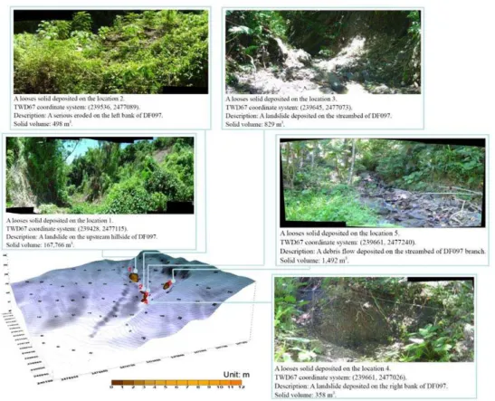
Field investigations in September 2006 discovered sev-eral locations with large amounts of deposit. The total solid volume exceeded 19 943 m3 distributed on the hillside and streambed of the watershed (Fig. 2). A total of 63.1 % of this material was located in regions with a slope greater than 15◦, and 7.8 % of the material was located in regions with slope less than 6◦. The formation of the mixture was composed of slate, mudstone, sandstone and weathered gravel, which are all easily movable under external forces.
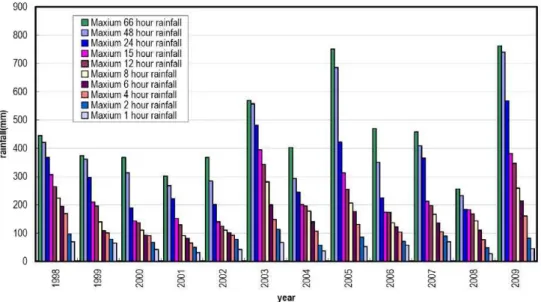
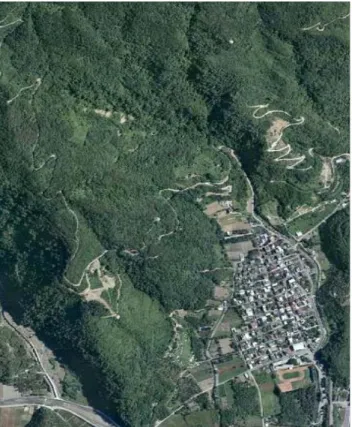
Typhoon Morakot struck Taiwan in August 2009 and pro-duced heavy rainfall. The maximal rainfall intensity of this event reached 45.5 mm h−1 (Fig. 3), and accumulated 759 mm of rainfall in 66 h (from 7 August 2009 at 9:00 a.m. to 9 August 2009 at 11:00 p.m.). The annual record for the maximal rainfall accumulated at 1, 2, 4, 6, 8, 12, 15, 24, 48, and 66 h duration are shown in Fig. 4. On 9 August 2009 at 3:00 p.m. (with a rainfall accumulation of 740.5 mm in 62 h), the rainfall induced considerable landslides and debris flows. The aerial photography after the disaster is shown in Fig. 5. Field investigations after the disaster revealed that almost 17.2 % (0.1485 km2) of the watershed was buried, the total volume of debris flow exceeded 500 000 m3, and almost 200 000 m3flowed out of the valley. The aerial photography before and after Typhoon Morakot are shown in Figs. 6 and 7, respectively, for comparison.
3 DEBRIS-2D model
The original O’Brien and Julien (1985) rheological relation-ship from a one-dimensional version was extended to a three-dimensional version, as follows:
τij= τ0 γ˙ij
+µd+µcγij˙ !
˙ γij, τij
> τ0 (1)
γ˙ij
=0,
τij
< τ0 (2)
whereτij is the shear stress tensor andγ˙ij is the strain rate tensor.τ0is the yield stress,µdis the dynamic viscosity and µcis the turbulent-dispersive coefficient.
τij
and
γ˙ij
A
B
C
DF097
Daniao tribe
Fig. 1.Stream DF097 watershed (at which the Daniao tribe debris flow occurred).
Fig. 3.Rainfall intensity recorded for Typhoon Morakot.
Fig. 4.Annual record for maximal rainfall accumulated for 1, 2, 4, 6, 8, 12, 15, 24, 4 and, 66 h duration in the DF097 stream watershed.
that most of the flow region was in a weak stress condition, that is, the plug region. The corresponding constitutive law is shown in Eq. (2), which can be expressed as follows:
γ˙ij
=
s
2∂u ∂x
2
+2∂v ∂y
2
+2∂w ∂z
2
+(∂u ∂y+
∂v ∂x)
2+(∂u
∂z+ ∂w ∂x)
2+(∂v
∂z+ ∂w ∂y)
2
=0, τij
< τ0 (3)
where thex-axis coincides with the averaged bottom of the channel and is inclined at angleθwith regard to the horizon. They-axis is in the transverse direction and thez-axis is per-pendicular to both thex- andy- axes.u,v,ware the velocity
components in thex,y,zdirections, respectively. Because debris flow in a lab or in the field is usually considered long waves, that is, the depth scale is substantially smaller than the horizontal length scales; it can be obtained from Eq. (4) by neglecting the small terms, as follows:
∂u ∂z=0,
∂v
∂z=0 (4)
Fig. 5.Aerial photography of Daniao tribe debris flow in Typhoon Morakot.
Substituting Eq. (4) into the momentum equations obtains the following:
∂u ∂t +u
∂u ∂x+v
∂u ∂y= −
1 ρ
∂p
∂x+gsinθ+ 1 ρ
∂τzx
∂z (5)
∂v
∂t +v ∂v
∂x+v ∂v
∂y= − 1 ρ ∂p ∂y+ 1 ρ ∂τzy ∂z (6)
0= −1 ρ
∂p
∂z−gcosθ (7)
whereρ is density of debris flow, andp is pressure. The stress free condition is applied at the free surface z= h(x,y,t ). The upper boundary of the thin boundary layer near the bottom is defined asz=B(x,y,t )+δ(x,y,t ), where the natural bottom of the debris flow isz=B(x,y,t ). Be-cause the thickness of the boundary layer is small compared to the flow depth, the natural bottom can be used as the boundary for the plug flow. Equation (7) leads to static pres-sure inz.
p=ρgcosθ (h−z) (8)
Integrating Eqs. (5) and (6) inzfrom the bottom to the free surface obtains the results in conservative form as follows: ∂uH
∂t + ∂u2H
∂x + ∂uvH
∂y = −gcosθ H ∂(B+H )
∂x +gsinθ H− 1 ρ
τ0u
√
u2+v2 (9)
∂vH ∂t +
∂uvH ∂x +
∂v2H
∂y = −gcosθ H ∂(B+H )
∂y − 1 ρ
τ0v
√
u2+v2 (10)
The depth integration of continuity equation gives ∂H
∂t + ∂uH
∂x +
∂vH
∂y =0 (11)
Fig. 6.Aerial photography before Typhoon Morakot.
4 Daniao tribe debris flow simulation
From the 2006 survey, we discovered that at least 20 000 m3 solid sources of debris flow were deposited on the triggering areas of the Daniao tribe watershed. However, for a heavy rainfall event, more material can be created. Therefore, we used a different approach by using accumulated rainfall to es-timate the volume of debris flow in this site. An equilibrium concentration conceptual of Takahashi (1980) was applied to estimate the debris flow volume. Takahashi (1980) derived the equilibrium concentration, as follows:
C∞= ρwtanθ
(ρs−ρw)(tanφ−tanθ )
(13) whereC∞is the equilibrium concentration, ρs is the solid density of debris,ρwis the liquid density of debris,φis the rest angle of solids, andθis the slope. In general,ρw is the water density,ρsandφmay be measured from field samples, andθmay be calculated from the Digital Topographic Model (DTM). In the Daniao tribe debris flow watershed (Taitung DF097 watershed), the slope was calculated from the average creek bottom slope as 23.2 % (≈13◦), as shown in Fig. 8.
From the field samples, the solid density was ρs = 2.6 g cm−3, andφ≈30◦. With the liquid density of ρw= 1.0 g cm−3, the equilibrium concentration was calculated as C∞=41.6 % from Eq. (13). The amount of water required
Fig. 7.Aerial photography after Typhoon Morakot.
Fig. 8.Average slope of the debris flow path.
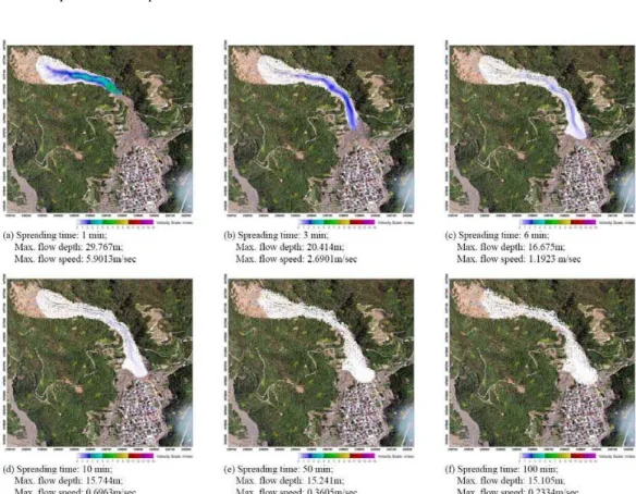
Fig. 9.The debris flow depth contour maps at various times.
Fig. 11. Region marked in red is the area affected by Typhoon Morakot, and the region marked in blue is the simulation result. The red star indicates where field depth estimation is available. The depth estimated by rescuers is between 12 m and 13 m. The simulated result for 508 417 m3is 13.06 m.
(A) Initial volume is 200,000 m3 (B) Initial volume is 300,000 m3
(C) Initial volume is 400,000 m3
(D) Initial volume is 500,000 m3
2
Max. Depth Front Peak Max. Depth
Front Peak
Max. Depth Front Peak
Max. Depth Front Peak
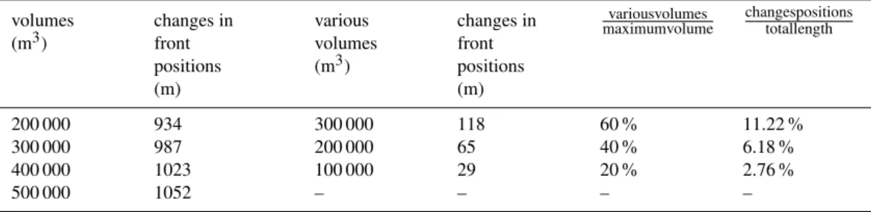
Table 1.Changes in front positions for various volumes.
volumes (m3)
changes in front positions (m)
various volumes (m3)
changes in front positions (m)
variousvolumes maximumvolume
changespositions totallength
200 000 934 300 000 118 60 % 11.22 %
300 000 987 200 000 65 40 % 6.18 %
400 000 1023 100 000 29 20 % 2.76 %
500 000 1052 – – – –
1
Fig. 13.Compared hazard zones in various volumes.
satisfied in 22.3 return years, based on frequency analysis. Therefore, a water volume accumulation of approximately 296 916 m3occurring in 62 h by using rational formula can be determined from the flow duration curve, and the debris flow volume of 508 417 m3may be determined from the wa-ter volume divided by (1-C∞). With all of the uncertainties, 508 417 m3can be considered the maximal possible amount. The DEBRIS-2D model was applied to assess a hazard zone. A yield stress of the debris flow of 250 dyne cm−2was mea-sured in the field. A time step of 0.01 s was set up, and the computational grid size was 5 m×5 m DTM of the Daniao tribe watershed. The initial debris sources were distributed at the head of the Taitung DF097 stream.
The following simulation results are for total volume of 508 417 m3. The simulated debris flow depth contour and velocity vector at 1, 3, 6, 10, 50 and 100 min are shown in Figs. 9 and 10. The maximal depth of the deposits was in excess of 15 m. The sources of debris flows were dis-tributed in the gap of the watershed (in the medium stream)
and flowed out of the valley region (in the down stream), as shown in Fig. 9a, b. The maximal velocity was in excess of 20 m s−1 during the start of the debris flow, however, it began to slow rapidly when the debris flow passed the wa-tershed gap (maximal velocity less than 3 m s−1), as shown in Fig. 10b, c, d and e. The results indicated that at approx-imately 10 min, the debris flow reached upstream of the Da-niao tribe, as shown in Figs. 9d and 10d. As the velocity of the debris flow slowed to less than 0.5 m s−1, as shown in Fig. 10f, the debris flow front peak continued to maintain the same depth (≈15 m), as shown in Fig. 9d, e and f. The final deposition fronts for all 4 cases are almost identical. The fi-nal deposition area for both the simulation and the real event are shown in Fig. 11. The simulation results were nearly con-sistent to the field measurements. However, drainage ditches were constructed on both sides of the village after the sim-ulation in 2006, therefore, a part of the debris flow spread along the ditches (Fig. 11). Consequently, the front travelled a shorter distance than that in the simulation because the only difference for various total volumes is the front location. The location for the maximum as predicted by numerical simula-tion is 3 m away from the real locasimula-tion, as shown in Fig. 11. A depth near the front of the field is available by the esti-mation from rescuers. The estimated depth is between 12 m and 13 m at the location marked by a red star in Fig. 11. The simulation result is 13.06 m for 508 417 m3.
12 m and 13 m at the location marked by a red star in Fig. 11. The simulation result is 13.00 m for 500 000 m3and 11.74 m for 200 000 m3.
This study compared hazard zones in various volumes, as shown in Fig. 13, and the front positions change for various volumes, as shown in Table 1. This study revealed that a 20 % variation in estimating the volume results in a 2.76 % variation on the final deposition front. This case study of the Daniao tribe debris flow provides support for the usability of numerical simulations in real engineering detailed designs.
5 Conclusions
This study used a DEBRIS-2D model to simulate a real debris flow event before it occurs. The location of loose deposits was discovered through a field investigation. The total volume was obtained through hydrological methods and was verified with field estimation. The simulated result obtained in 2006 had a deposition area that was nearly consistent to the real event in 2009. The maximal depth and its location does not have a practically meaningful error between the numerical result and real event. The relative insensitivity from volume estimation is one reason for this successful prediction. Because of the limited watershed terrain, the hazard zones of debris flows were not expanded. This study revealed that a 20 % variation in estimating the volume results in a 2.76 % variation on the final deposition front. This case study of the Daniao tribe debris flow provides support for the usability of numerical simulations in real engineering detailed designs.
Edited by: M. Arattano
Reviewed by: T. Mizuyama and another anonymous referee
References
Coussot, P., Proust, S., and Ancey, C.: Rheological interpretation of deposits of yield stress fluids, J. Non-Newton. Fluid, 66, 55–70, 1996.
Coussot, Ph.: Mudflow Rheology and Dynamics, Publisher, Taylor and Francis Group, 1997.
Coussot, Ph. and Proust, S.: Slow unconfined spreading of a mud flow, J. Geophys. Res., 101(B11), 25217–25229, 1996.
Engrg., 117, 346–353, 1991.
Liu, K. F. and Lai, K. W.: Numerical simulation of two-dimensional debris flows, Proceedings of the 2nd International Conference on Debris Flow Hazards Mitigation, 531–535, 2000.
Liu, K. F. and Hsu, Y. C.: Study on the sensitivity of parameters relating to debris flow spread. Proceedings of the International Conference, Debris Flows: Disasters, Risk, Forecast, Protection, Pyatigorsk, Russia, 19–22, 2008.
Liu, K. F. and Huang, M. Ch.: Numerical simulation of debris flow with application on hazard area mapping, Comput. Geosci., 10, 221–240, 2006.
Liu, K. F. and Mei, C. C.: Slow spreading of the sheet of Bingham fluid on an incline plane, J. Fluid Mech., 207, 505–529, 1989. Liu, K. F. and Mei, C. C.: Roll waves on a layer of a muddy fluid
flowing down a gentle slope – A Bingham model, Phys. Fluids, 6, 2577–2590, 1994.
Liu, K. F., Li, H. C., and Hsu, Y. C.: Debris flow hazard assessment with numerical simulation, Nat. Hazards, 49, 137–161, 2009. Mei, C. C., Liu, K. F., and Yuhi, M.: Mud flow-slow and fast, Lect.
Notes Phys., 582, 548–577, 2001.
Ng, Ch. O. and Mei, C. C.: Roll waves on a shallow layer of mud modelled as a power-law fluid, J. Fluid Mech., 263, 151–184, 1994.
O’Brien, J. S. and Julien, P. Y.: On the importance of mudflow routing, Proc., 1st Int. Conf. on Debris-Flow Hazards, Mitiga-tion: Mechanics, Prediction and Assessment, ASCE, Reston, Va., 677–686, 1997.
O’Brien, J. S. and Julien P. Y.: Physical properties and mechanics of hyperconcentrated sediment flows, Proc. ASCE Hyd. Div. Spec. Conf. on Delineation of Landslides, Flash Flood and Debris Flow Hazards, Logan Utah, June 1984, 260–279, 1985.
Osmond, D. I. and Griffiths, R. W.: The static shape of yield strength fluids slowly emplace on slope, J. Geophys. Res., 106(B8), 16241–16250, 2001.
Pouliquen, O. and Forterre, Y.: Friction law for dense granular flows: application to the motion of a mass down a rough inclined plane, J. Fluid Mech., 453, 133–151, 2002.
Takahashi T.: Debris flow on prismatic open channel, J. Hydr. Div., 106, 381–396, 1980.
Wieland, M., Gray, J. M. N. T., and Hutter, K.: Channelized free-surface flow of cohesionless granular avalanches in a chute with shallow lateral curvature, J. Fluid Mech., 392, 73–100, 1999. Wilson, S. D. R. and Burgess, S. L.: The steady, spreading flow of