Regional Subsidies and Industrial Prospects of Lagging Regions
by
Alexandre Carvalho
DIRUR,Instituto de Pesquisa Econômica Aplicada (IPEA) alexandre.ywata@ipea.gov.br
Somik V. Lall
Development Research Group, The World Bank slall1@worldbank.org
Christopher Timmins
Department of Economics, Duke University timmins@econ.duke.edu
ABSTRACT
Large and sustained differences in economic performance across regions of developing countries have long provided motivation for fiscal incentives designed to encourage firm entry in lagging areas. Empirical evidence in support of these policies has, however, been weak at best. This paper undertakes a direct evaluation of the most prominent fiscal incentive policy in Brazil, the Fundos Constitucionais de Financiamento (Constitutional Funds). In doing so, we exploit valuable features of the Brazilian Ministry of Labor's RAIS data set to address two important elements of firm location decisions that have the potential to bias an assessment of the Funds: (i) firm “family structure” (in particular, proximity to headquarters for vertically integrated firms), and (ii) unobserved spatial heterogeneity (with the potential to confound the effects of the Funds). We find that the pull of firm headquarters is very strong relative to the Constitutional Funds for vertically integrated firms, but that, with non-parametric controls for time invariant spatial heterogeneity, the Funds provide statistically and economically significant incentives for firms in many of the targeted industries.
JEL Classification: L22, R12, R58
Acknowledgements
1. INTRODUCTION
Sub-national disparities in economic performance and living standards are large
and often sustained in many countries. Prospects for lagging regions in developing
counties are of particular concern as these areas are not just characterized by lower relative
incomes and standards of living, but may in fact be home to significant incidence of
absolute poverty. Local populations may be stuck in so-called spatial poverty traps, in
which poor infrastructure and resource endowments limit access to educational, social, and
economic opportunities (Jalan and Ravallion 1997).
Many governments have opted for interventions to offset these disparities, actively
intervening to promote capital flows and fiscal transfers designed to support incomes or to
subsidize the creation of jobs and the extension of credit. These incentives should offset
costs of firm location that may arise due to higher transport and logistics costs, poor
infrastructure conditions, factor price differentials, and lower levels of public services and
amenities. Tax holidays and interest rate subsidies have been used to develop an
autonomous industrial base in the Northeast of Brazil; financial concessions and
investment subsidies (along with industrial estates and preferential industrial licensing)
were used to stimulate growth in backward regions of India; reductions in import duties,
taxes (income, sales, and capital gains), and interest rates were used to move industry out
of the largest urban areas in Mexico; and extensive tax holidays were used as an incentive
for firms in Thailand to move out of Bangkok into regional cities.
In most countries, there is little evidence that decades of spatially explicit
interventions have led to improved economic performance and welfare enhancements in
have enhanced national welfare. Is it welfare enhancing to move a firm from one location
to another and then pay for its re-location costs? Do these policies encourage any new
entry, or do they simply result in the spatial re-allocation of firms that would have entered
anyway? In this paper, we outline a strategy to evaluate the simplest impacts of spatially
explicit development programs using data from the Brazilian Constitutional Funds – one of
the largest regional incentive policies in the world.
1.1 Regional Disparities in Brazil
Brazil has a long history of regional disparities. The Brazilian Northeast has
historically been the poorest region in the country, with regional per capita incomes being
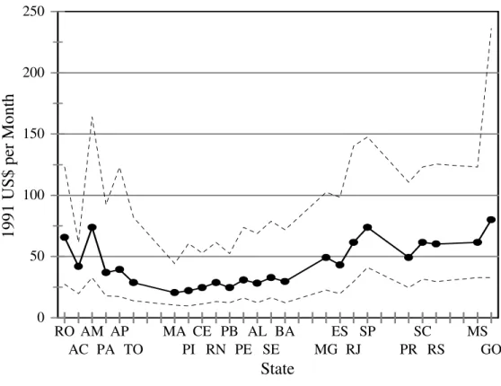
about one half of those in the prosperous Southeast (Lall and Shalizi, 2003). Figure 1
describes the 25th, 50th, and 75th percentiles of the Brazilian monthly income distribution by state based on 1991 demographic census data (state abbreviations defined in Table 1).
The highest median per capita household income ($79.93 per month in Goias) is nearly
four times larger than that of the lowest median per capita household income state ($20.49
per month in Maranhao). Eight states report median per capita household incomes of less
than $1 per day, seven of which are located in the country’s Northeast region. Of the ten
poorest states in the country, eight are in the Northeast, and two in the North region
(Azzoni et. al, 2002). These large per capita income differences across regions are,
moreover, surprisingly stable over very long periods. Per capita income in the Southeast
was 2.9 times that of the Northeast in 1939 and 2.8 times in 1992 (World Bank, 1998).
Beyond purely economic indicators, social indicators in the Northeast region are
higher than that of São Paulo, the child mortality rate is twice as large as that of the
Southeast (54.5 per thousand in the Northeast compared to 26.3 per thousand in the
Southeast), life expectancy four years shorter, and income inequality is much worse
(Ferreira, 2004). Inequality, measured by the Theil coefficient is 0.80 for Ceará, Bahia and
Pernambuco, in contrast to 0.55 for the state of São Paulo (Ferreira, 2000). Fifty percent
of the Northeast population lives in poverty.
1.2 Regional Development Policies in Brazil
Large regional disparities between the Northeast and the rest of the country
(coupled with a severe drought in 1958) stimulated the Brazilian government to develop
explicit policies for that region (Baer, 1995). The strategy was to establish an autonomous
center of manufacturing expansion by attracting “dynamic” and high-growth industries,
such as those in metallurgy, machinery, electrical equipment and paper products (World
Bank, 1987). Instruments such as fiscal incentives, transfers, and direct expenditures in the
form of industrial land and infrastructure were widely used to attract economic activity
(Goldsmith and Wilson, 1991; Markusen, 1994; World Bank, 1987).
Financial outlays from the central government in Brazil to support spatially explicit
programs have been estimated to be US $3 to 4 billion per annum in recent years (Ferreira
2004). The estimated cost of tax breaks and associated regional development programs
(excluding the Zona Franca de Manaus) in 2002 was estimated at almost US $900 million
(Secretaria da Receita Federal, 2003). Tax credits directed to the Zona Franca de Manaus
are estimated to be US $1.2 billion in 2003 alone. Investment incentive programs for the
million dollars a year between 1995 and 2000, before they were shut down over
accusations of mismanagement.
The main objective of our paper is to examine the effect of regional subsidies on
industrial prospects of lagging regions in Brazil. There have been several reviews of
spatially explicit programs in Brazil and also in other countries, with the general
conclusion that these initiatives have very small effects. For instance, Ferreira (2004)
claims that much of the GDP per capita growth in the Northeast (and convergence with the
South and Southeast) can be attributed to out-migration rather than local employment
creation, and that welfare gains from these interventions are limited as most of the
population that benefited from the jobs created came from other parts of Brazil. He also
finds that most of the convergence in per capita incomes across Brazilian regions occurred
over the period 1970-1985, before the initiation of the Constitutional Funds. [Ellery and
Ferreira (1996)] Maia Gomes (2002) finds that, while GDP did grow throughout Brazil
over the period 1960 to the present, it did not grow as fast in the Northeast (the focus of
most regional policies) as in the rest of the country. Ferreira (2004) finds similar results
focusing only on the period 1990-2000 (i.e., the first decade of the Constitutional Fund
program).
Each of these papers looks for indirect evidence of regional policies’ impacts on
economic outcomes (e.g., GDP or GDP growth rates). The problem with this approach is
that these outcomes are affected by a multitude of factors besides regional policy (e.g.,
macroeconomic shocks), some of which may influence certain parts of the country more
than others. The relevant question is not whether the Northeast grew faster than the rest of
it would have in the absence of the program. This is a very difficult question to answer. In
this paper, we instead conduct a more direct evaluation of the impact of the Constitutional
Funds. In particular, we address a relatively limited question – did the Constitutional
Funds successfully induce entry by firms into Brazil’s lagging regions? Answering this
question necessarily precedes and motivates further work on measuring the welfare
impacts of the policy (which we outline in the conclusion). In addressing this question, we
account for two features of the firm location problem that have the potential to bias
estimates if ignored. First, we non-parametrically account for regional attributes such as
amenities, infrastructure, local public goods, and natural endowments. Since regional
incentives are allocated to compensate for inter-regional differentials in local
characteristics, it is imperative to adequately account for these factors in examining the
contribution of these programs. Otherwise, there is a tendency to systematically understate
their value. Second, our empirical analysis makes use of a linked headquarter-branch plant
panel data set, which allows us to consider the role of intra-firm considerations in the
location decisions of vertically integrated firms. If firms tend to locate branch plants in
close proximity to their headquarters, and if those headquarters are disproportionately
located in unsubsidized areas, this could be mis-interpreted as a failure of the fiscal
incentive. While the empirical application focuses on Brazil, the estimation strategy
outlined in the paper has broader applicability and can be used to examine similar issues
across countries.
Our main findings are that subsidized credit offered to firms via the CF’s has
worked in terms of industrialization in the Northeast. At the same time, we find that pull
vertically integrated firms (i.e., with headquarters). This implies that, for vertically
integrated industries, firm structure needs to play a part in the CF – i.e., reform to promote
entry by headquarter firms into lagging regions. In more footloose sectors, such reforms
would not be necessary.
The remainder of this paper is organized into five sections. In Section 2, we
discuss the design and allocation of the CF’s. Section 3 describes the data, and Section 4
discusses our estimation strategy. Section 5 describes the main findings and Section 6
concludes.
2. ALLOCATION OF BRAZILIAN CONSTITUTIONAL FUNDS
National governments in many countries have a long history of using fiscal
incentives to stimulate the growth potential of lagging sub-national regions. These
spatially explicit programs are designed to compensate for location specific disadvantages,
such as transport and logistics costs, infrastructure conditions, factor price differentials and
lower levels of public services and amenities. A detailed discussion on various regional
development programs in Brazil is provided in Ferreira (2004) and World Bank (2005).
Explicit spatial policies in Brazil include three sets of instruments which target private
sector development through various kinds of subsidies: (a) fiscal incentive programs such
as those administered by SUDENE, SUDAM, and the Zona Franca de Manaus (Manaus
Free Trade Zone); (b) subsidized credit channeled through the CF’s, which has become one
of the most important instruments of spatial policy in Brazil; (c) and regional development
banks, such as Banco do Nordeste do Brazil (BNB).
through the CF’s. In 1989, the Brazilian Congress instituted three Constitutional
Investment Funds (Fundos Constitucionais de Financiamento) for the Northeast (FNE), the
Center-West (FCO), and the North (FNO). The main aim of these funds was to stimulate
economic and social development in these regions by extending credit to local
entrepreneurs. Preferential treatment was provided to micro- and small-scale agricultural
producers and small-scale manufacturing to encourage the use of local raw materials and
labor. Sixty percent of the outlays for the CF’s were allocated to the Northeast, and 20
percent were allocated to each of the North and the Center West. Funds are transferred
from the National Treasury to the Ministry of Integration (“Ministério da Integração”),
which later reallocates them to the operating banks – the Banco do Nordeste (FNE), Banco
da Amazônia (FNO) and Banco do Brasil (FCO). The CF’s are financed by receipts from
income taxes and taxes on industrial products.
Interest rate subsidies are the main incentive offered through the CF’s. While
market interest rates offered to private firms are currently more than 45%, the CF’s offer
credit at 8.75% to non-agricultural micro firms; 10% to small firms, 12% to medium sized
firms; and 14% to large enterprises. Interest rates are even lower for comparable agro
producers: 6% for mini-producers, 8.75% for small to average and 10.75% for large ones.
These interest rates were negative in real terms in 2002, when inflation was 12.5%. Rates
offered to individual producers varied by sector, investment size, and credit record of the
borrower. Between 1989 and 2002, more than US $10 billion were provided in subsidized
3. DATA
We compile a database that maps the spatial entry decisions of new establishments
in Brazil, with the goal of learning how the CF’s affect those decisions. The main source
of information is the RAIS micro data, provided by the Labor Ministry.1 We study the effects of the CF’s on entry by firms in 18 sectors (11 manufacturing and 7 service, which
are listed in Table 2) into 265 “urban agglomerations” (see description below) over the
years 1993-2001. The RAIS database contains a wide range of information for all
economic establishments in the formal sector in Brazil from 1986 onward. For each
establishment in this database, we have annual information on the number of employees at
the beginning and end of each year; total salaries and wages; in which municipality the
company is located; as well as the establishment’s economic activity according to several
industry classifications. To avoid problems caused by a large number of establishments
with very few employees, we limit our analysis to establishments with no fewer than 10
employees. This paper is the first research project to use the RAIS data to study firm
geography and the effectiveness of fiscal incentives.
As discussed above, one important piece of information in the estimated models is
the composition and location of the “relatives” for each establishment. To uncover the
composition of each family of establishments (parent and sibling establishments), which
constitutes a firm, we make use of the establishment identification number, hereafter
CNPJ. The CNPJ has 14 digits and is the official identification number for all productive
units in the formal sector. The first 8 digits of the CNPJ indicate the company (or family)
of each establishment. The next 4 digits indicate the position of the establishment in the
1
family. For example, “0001” indicates the first establishment in the company, which is
assumed in this paper to be the company headquarters. The other establishments in the
company are given sequential codes, so that the second establishment receives “0002”, the
third establishment receives “0003”, and so on. Some of the companies are comprised of a
single establishment, which receives the 4-digit code “0001”.2 The last two digits of the CNPJ correspond to the establishment economic sector, and they work more as a
confirmation code. Therefore, we use the first 12 digits of the CNPJ to extract the
establishment composition of each company.
To summarize, there are three reasons why the RAIS data set is particularly useful
for the analysis. These are:
(i) It identifies entry behavior each year, allowing us to build a panel of entry data that we use to control for spatial fixed effects.
(ii) It provides spatial detail on entry decisions (necessary for discussion of policies to promote entry into lagging regions).
(iii) It describes firm family structure (i.e., identifies parent or headquarters, which we find to be a particularly important determinant of entry).
To model spatial entry decisions, we had to select an appropriate geographic unit.
Using municipalities creates several problems: (i) there are a large number of
municipalities (5,506 in the year 2000), which would significantly increase the
computational burden in estimating the location decision model; (ii) many municipalities
2
are very small (i.e., with fewer than 5,000 inhabitants) and/or in rural areas with very few
establishments in the formal sector; (iii) because of the continuous creation of new
municipalities in Brazil, it is necessary to coordinate different municipality maps across the
years of study; and (iv) entry into municipalities within the same urban area is likely to be
highly correlated. Given these problems, we decided instead to use the concept of “urban
agglomerations,” defined in a comprehensive urban study developed by IPEA, IBGE and
Unicamp (2002), and used by Da Mata, Deichmann, Henderson, Lall and Wang (2005a
and 2005b).
Even though RAIS micro data are available from 1986 to 2003, the data from 1993
to 2001 contain fewer missing observations and are considered to be generally more
reliable. We therefore use only these years for the analysis. For each year, we identify
new establishments with at least 10 employees and record the urban agglomeration in
which they entered. If the entering establishment belonged to a multi-establishment firm,
we also identify the urban agglomeration of the parent.
As can be noted from Table 1, most parent establishments are located in the
Southeast (58.15% in 1993). Note, however, that the percentage of entering parent firms
over the period 1993-2001 (i.e., the CF years) falls to 42.7% in the Southeast, but rises to
21.01% in the Northeast (from 12.49% of the parents in 1993). Thus, considering only the
spatial distribution of parents (which are footloose by definition), there is some evidence
that the CF’s were effective. There is also evidence in this table, however, that if branches
are closely tied to parents, the CF’s have a lot to overcome in vertically integrated
industries, given the initial distribution of parent firms in 1993.
upon the sector being considered. Table 2 shows percentage of entrants over years
1993-2001 that have headquarters. We would expect proximity to the parent to be particularly
important for Metallurgy, Communcations and Electronics, Transportation, Chemicals, and
Shoes. Table 2 also shows the average distance branch plants locate from headquarters
(conditional on having a headquarters). These numbers are very small, providing further
evidence that the pull of the parent is significant.
4. ESTIMATION STRATEGY
Our estimation strategy is designed to answer the following questions: (i) were the
CF’s effective in inducing firms to locate new establishments in Brazil’s lagging regions,
(ii) what role does the spatial distribution of a multi-unit firm play in the location decision,
and (iii) what local attributes are important factors in firms’ location decisions. In
answering these questions, we face a number of challenges. First among these is
separating the role of idiosyncratic firm characteristics from those of local attributes and
CF allocations. In particular, in deciding where to place a new branch plant, a multi-unit
firm may take into account proximity to the firm’s headquarters. The location of each
firm’s headquarters will be unique, and it is unclear a priori in what direction ignoring this
factor would bias our conclusions.3
Second, we must separate the role of the CF subsidies from that of unobserved
local attributes. The CF is a subsidy to promote entry into lagging regions. Regions with
high subsidies are therefore likely to be unattractive for entry in a variety of other
3
dimensions. Data to control parametrically for these other factors are incomplete, creating
a problem of (negatively) correlated unobservables. We exploit useful features of the
RAIS data set to control for this problem with agglomeration fixed effects.
Finally, in determining the role played by other factors in the entry decision (e.g.,
classical determinants like transportation cost and market size, along with agglomeration
effects and other forms of local spillovers), we are confronted with problems of severe
multicollinearity. In Brazil, development (as measured by the IDH) is highly correlated
with measures of education, infrastructure (e.g., sewage, electrification), and even transport
accessibility. This will limit our ability to deduce the separate causal role of many of these
factors.
In dealing with these complications, we undertake a two-stage estimation
procedure. The following sub-sections describe each of these stages. The next section
provides a discussion of the results.
4.1 Stage #1: Maximum Likelihood Entry Model
In the first stage, we recover non-parametric estimates of each agglomeration’s
overall attractiveness for entry (separately for each sector), taking into account the
possibility that a firm might consider the proximity of the new site to its headquarters.
Ceteris paribus, we should expect firms to dislike locating their plants long distances from
the parent. The magnitude (and even sign) of this effect, however, may differ by sector.
We model the payoff to an entering plant i (part of firm k in industry m) from
locating in agglomeration j in year t as:4
4
(1) i jkt ijkt m t m t j m t k j
i, , , =δ , + β D, , , +η, , ,
Π
where
m t j,
δ = fixed effect capturing all features of agglomeration j in period t, as perceived by a potential entrant in industry m5
Di,j,k,t = distance (km) to the parent of plant i from location j in year t ( = 0
if no parent)
i,j,k,t = unobserved idiosyncratic features of location j in year t specific to
plant i from firm k
We take the set of all entering firms in each year as given and model their entry decision
over the set of all locations.6 Assuming ηi,j,k is distributed i.i.d. Type I Extreme Value,
the probability that plant i enters agglomeration j in year t is given by:
(2) = + + = J l t k l i m t m t l t k j i m t m t j m t k j i D EXP D EXP P 1 , , , , , , , , , , , } { } { β δ β δ
research has found that larger firms may be more responsive to local variables in a model of spatial entry, either because of economies of scale in spatial search or because smaller firms may be more tied to the home of the entrepreneur. (Levinson 1996)
5
At this stage of the model, m t j,
δ can be assumed to control for a wide variety of local attributes including (but not limited to) indicators of development (e.g., sewage, electrification, piped water), measures of transportation accessibility (e.g., cost of transporting freight to Sao Paulo), the education and income of the local population (e.g., average education of the population over age 25, illiteracy rate), market size (i.e., population, income), and spillovers with other firms (both within and across sectors).
6
The likelihood of the observed data (defined separately for each industry m and year t) is
thus given by:
(3)
∏∏
∈ = = m i J j m t k j i m t m t m t m t t j i P D L 1 , , , , , ] [ ) , ;
( β δ λ
where i,j,t = 1 if plant i sites in urban agglomeration j in year t ( = 0 otherwise).
Maximizing this expression yields estimates of m t
β and m
t
δ .7
A practical difficulty arises in this stage of the estimation. In particular, some
urban agglomerations may not be entered by any plants in an industry in a particular year.
The data, therefore, reveal only that these locations are inherently undesirable, but do not
indicate just how undesirable. The fixed effects m t j,
δ are not identified for these locations.
This is fundamentally a problem of censored data. Unlike traditional approaches to this
problem (which rely on strong distributional assumptions), we solve it by ascribing a very
small minimum artificial number of entrants (e.g., 10-6) to each agglomeration – a numerical “patch”. Depending upon how small of a patch is assumed, the estimated values
of m t j,
δ for each un-entered agglomeration can be arbitrarily negative. Timmins and
7
Explicitly maximizing the likelihood function in (3) over the full vector of fixed effects δtm may prove computationally difficult. We therefore employ the contraction mapping proposed by Berry (1994) and used in Berry, Levinsohn, and Pakes (1995) to avoid this problem. Practically, we integrate over entrants i in equation (2), yielding expressions for the predicted share of plants in each sector choosing to locate in each agglomeration in each year. Given a guess for the value of m
t
β , these expressions constitute a contraction mapping in the vector of δmj,t's. We use this mapping to find the unique set of s
m t j, '
δ that make the shares predicted by the model equal the actual shares within some acceptable level of tolerance. The likelihood function is calculated based on these m s
t j,'
δ . The parameter m
t
β is updated in such a way as to increase that likelihood value, and the contraction mapping is repeated in order to recover new m s
t j, '
Murdock (2006) demonstrate that, as the patch size becomes increasingly small, the
estimated values of m t j,
δ for those urban agglomerations that are entered converge to stable
values. As long as a majority of agglomerations are entered by each sector, median
regression used to recover the determinants of m t j,
δ will be unaffected by the artificially
assumed number of entrants in un-entered agglomerations.8
4.2 Stage #2: Median Regression and the Role of the Constitutional Funds
In order to evaluate the role of the CF’s in promoting entry, we use median
regression on the panel of data (defined over J = 265 agglomerations and T = 9 years) for
each industry.9
(4) m
t j t j m m j m
t m
m t
j, =γ +YEAR′θ + AGG′ φ +ψ CF, +u ,
δ
where
t
YEAR = vector of dummy variables indicating year t = 1994, …, 2001 (1993 excluded)
t
AGG = vector of dummy variables indicating agglomeration j = 2, …, 265 (agglomeration j = 1 excluded)
CFj,t = average CF allocation per employee in year t in the state containing agglomeration j10
8
See Koenker and Basset (1978) and Koenker and Hallock (2001) for comprehensive discussions of median regression.
9
Note that estimating this equation via median regression requires explicit estimation of all fixed effects – differencing the data is not equivalent to fixed effect estimation in the median regression context.
10
m t j
u , = unobservable determinant of entry quality in agglomeration j for firms in sector m in year t
The vector of year dummies is included to account for the fact that an arbitrary
normalization underlies the vector of δtm in each year t (in particular, these fixed effects
have no natural scale, so we normalize them so that their average values equal zero in each
year for each industry).
The vector of agglomeration dummies plays an especially important role in this
regression. In particular, CF’s are allocated in a remedial fashion (i.e., with more funds
being allocated toward locations that are less attractive for entry).11 A regression of m t j,
δ
on only year dummies and CF allocations therefore suffers from an omitted variable bias –
in particular, a bias towards finding that the CF’s had no impact (or even an adverse
impact) on entry behavior. With only cross-sectional data, one would be forced to deal
with this fact by including as many agglomeration attributes in the model as possible.
While such data exist, they will necessarily be incomplete. With our panel data (obtained
by using annual entry behavior observed in the RAIS), we are able to control
non-parametrically for any features of each agglomeration that do not change over time. This
year. This converts our measure of CF’s into the average contracted allocation per employee in each state, which we treat as an exogenous measure of the state’s attractiveness in terms of the CF. Controlling for the sectoral composition of entering firms on our measure of the CF’s as well has no effect on the results that we report. Note one remaining potential source of bias – firms with better credit ratings will receive higher CF subsidies (conditional upon size). If firms with better credit ratings disproportionately locate in sites with desirable unobservables, the error in our CF measure will be correlated with those unobservables, biasing our results towards finding positive effects of the CF’s. We demonstrate below, however, that this potential source of bias is not a concern in interpreting our results.
11
takes care of the most important differences between agglomerations, and leaves us with
the variation in CF allocations over time with which to identify their impact.
5. RESULTS
5.1 The Role of Parent Location in Entry
Table 3 reports the results of our first stage estimates of m t
β for each of eighteen
sectors.12 In every instance, firms exhibit a statistically significant preference for siting their new plants close to their headquarters. In recovering these effects, Stage #1 of our
estimation strategy non-parametrically controls for everything about agglomerations that
varies by sector and year and that might be a determinant of firm entry. This should
control for the most important confounding factors (i.e., for any factor that makes it
attractive to put any firm from a particular sector – headquarters or otherwise – in the
agglomeration). It cannot distinguish, however, between distance effects and the effect of
idiosyncratic unobservables.13
While providing evidence of statistical significance, the parameter estimates in
Table 3 do not, however, allow us to judge the economic significance of the “pull” of the
firm headquarters in plant location decisions. In particular, in each of the maximum
likelihood procedures underlying the estimates reported in Table 3, there is a vector of
fixed effects normalized so that their average value equals zero. This normalization is
arbitrary, and makes direct comparison of parameter estimates across years or industries
impossible. More can be learned about the way in which these firm headquarters influence
12
Estimates of m t j,
entry behavior by way of simulation. In particular, it is possible to simulate how entry
patterns would have differed by sector and region if firms did not care about proximity to
headquarters. Assuming that the values of m t j,
δ are not affected by this counterfactual
assumption,14 we simply “turn off” the distance-to-parent coefficient in the entry model, and simulate new entry patterns in each year. Table 4 reports the percent change in the
distribution of entry (i.e., between actual and predicted under this counterfactual
assumption), across regions and aggregated over the years 1993-2001. The biggest
differences are seen in the North (i.e., where relatively few headquarters were in place in
any sector, but which sees the biggest gains when distance-to-parent effects are taken out)
and in the Southeast (i.e., the home to the majority of headquarters, which sees the largest
drop in entry). The Northeast, Center-West, and South see mixed effects that vary by
sector, although the general trend is for entry to increase in these sectors when we make all
plants “footloose”.
5.2 The Effectiveness of the Constitutional Funds
Table 5 describes our decomposition of the fixed effects, δmj,t. Columns describe
the results of median regressions that (i) exclude agglomeration fixed effects, using only
year fixed effects and annual CF contracts per employee, (ii) use year fixed effects and
annual CF contracts per employee along with a collection of covariates describing
13
For example, the model would interpret a case in which an entrepreneur has a strong preference for a particular agglomeration and locates all of his plants and headquarters there as a distaste for locating branch plants far from the headquarters.
14
observable agglomeration attributes,15 and (iii) use year fixed effects, agglomeration fixed effects, and annual CF allocations. In the table, we report only the coefficient on the CF
variable. Without any controls for agglomeration heterogeneity in column (i), we find
significant (both economically and statistically) negative effects of the CF on entry. This
result corresponds to that found in previous work (Ferreira 2004) and likely reflects the
fact that the CF’s are allocated in a remedial fashion. Including covariates in column (ii) to
control for local attributes does little to change these results.
Time-invariant forms of heterogeneity are non-parametrically controlled for by the
introduction of agglomeration fixed effects. These are included in the specification
described in column (iii), where we find significant positive effects of the CF’s on entry
for five out of the eleven manufacturing industries, and positive but insignificant effects
for all but paper and publishing and metallurgy (where effects are negative and
insignificant).
While the fixed effects succeed in alleviating the downward bias in the CF
parameters that is evident in columns (i) and (ii), keep in mind that there still may be some
remaining downward bias caused by time varying forms of local heterogeneity that are
negatively correlated with CF allocations. We are less concerned with the potential for
bias introduced by the mis-measurement of CF allocations resulting from the non-random
siting of plants according to their credit rating (see footnote 12). In particular, we would
expect that firms with more talented entrepreneurs would have better credit ratings and that
these entrepreneurs would be more likely to site plants in locations with desirable
15
unobservable attributes. This would tend to bias the coefficient on CF in our median
regressions upward. This source of bias should go down, however, when we introduce
agglomeration fixed effects to account for time-invariant forms of unobserved
heterogeneity. It is precisely when we introduce these fixed effects, however, that the sign
of most of our CF effects changes dramatically, switching from negative to positive.
Clearly, if there had been an upward bias in the absence of these fixed effects, it was not
very big and was swamped by the bias introduced by the correlation between CF and
undesirable unobservable local attributes.
Of the non-manufacturing sectors, only retail, transportation and communication,
and hotel and food services show positive effects from the CF’s. Non-manufacturing
sectors are generally not covered by the CF’s, so we should not expect to see the positive
effect here that we saw in the case of most manufacturing industries. Entry in the retail
sector, however, may quickly follow manufacturing entry and, hence, exhibit a positive
correlation with CF. In addition, the CF’s have been used to promote tourism related
activities, which may influence firm entry in the hotel and food services and transportation
and communication sectors (Ferreira 2004).
6. CONCLUSIONS
We learn two things from this analysis. First, (contrary to previous work) we find
that the CF allocations have, in fact, been successful in inducing entry into lagging regions,
conditioning on the location of firms’ headquarters. This result however, can be easily lost
among the confounding effects of local unobservables that are negatively correlated with
CF allocations. It is hard to capture these determinants of entry with available data
describing agglomeration attributes, and without properly accounting for these factors,
there is a bias toward finding a negative effect of the CF’s on entry. The RAIS data, which
describe spatial entry behavior on an annual basis, provide a unique opportunity to
overcome this problem non-parametrically.
Second, we learn that, while the CF’s were successful, headquarter proximity is a
significant determinant of entry behavior (conditional upon having a parent) that works to
offset this success. Simply “turning-off” the effect of parent firm location significantly
raises overall entry into lagging regions. These effects are, moreover, likely a lower bound
on the effect of removing the pull of firm headquarters if we believe that there are positive
spillovers between entrants.
The conclusions of this paper for policy-makers are, unfortunately, limited. While
we find that the CF’s were successful in inducing firms to locate in Brazil’s lagging
regions (and that the CF’s may yield more “bang for the buck” if they are used to induce
entry by firms’ headquarters into those regions), we are unable to determine with available
data whether the CF’s were good policy or not. In further research, we plan to move from
the limited (but important) question of “do subsidies affect firm location decisions” to the
more policy-relevant question of “are these subsidies welfare enhancing”. In answering
that question, it will be crucial to determine (i) whether the CF’s induced new entry into
lagging regions or simply re-allocated entry away from the South and Southeast regions,
and (ii) what was the productivity effect on re-located firms.16 Answering these questions was not possible with the data used in this paper, but may require new efforts in collecting
16
survey data from entrepreneurs about what motivated their entry decisions, and about their
inputs and outputs conditional upon those decisions.
REFERENCES
Azzoni, C. R., N. Menezes-Filho, T. A. de Menezes and R. Silveira-Neto (2002). “Geography and Income Convergence among Brazilian States”, Mimeo.
Baer, W. (1995). The Brazilian Economy: Growth and Development. 4th ed. Westport: Praeger.
Berry, S. (1994). “Estimating Discrete Choice Models of Product Differentiation.” RAND Journal of Economics. 25:242-262.
Berry, S., J. Levinson, and A. Pakes (1995). “Automobile Prices in Market Equilibrium.”
Econometrica. 63:841-890.
Da Mata, D., U. Deichmann, J.V. Henderson, S.V Lall and H. Wang (2005a). Determinants of City Growth in Brazil. IPEA Discussion Paper No. 1112. Brasília. 2005.
Da Mata, D., U. Deichmann, J.V. Henderson, S.V Lall and H. Wang (2005b). Examining the Growth Patterns of Brazilian Cities. IPEA Discussion Paper No. 1113. Brasília. 2005.
Ellery Jr. R. and Ferreira, P.C. (1996). “Crescimento Economico e Convergencia entre a Renda dos Estados Brasileiros.” Revista de Econometria. 16(1):83-104.
Ferreira, A.H.B. (2000). “Convergence in Brazil: Recent Trends and Long Run Prospects.”
Applied Economics. 32: 479-489.
Ferreira, P. C. (2004). “Regional Policy in Brazil: A Review.” Mimeo.
Goldsmith, W. and R. Wilson (1991). Poverty and Distorted Industrialization in the Northeast, World Development. 19(5):435-55.
Jalan, J. and M. Ravallion (1997). “Spatial poverty traps?” Policy Research Working Paper
No. 1862, Development Research Group, World Bank, Washington, D.C.
Koenker, R. and G. Bassett (1978). “Regression Quantiles.” Econometrica. 46(1):33-50.
Koenker, R. and K. Hallock (2001). “Quantile Regression.” Journal of Economic Perspectives. 15(4):143-156.
Lall, S. V. and Z. Shalizi (2003). “Location and growth in the Brazilian Northeast.”
Journal of Regional Science. 43(4):1-19.
Lall, S.V., R. Funderburg, and T. Yepes (2005). Location, Concentration, and Performance of Economic Activity in Brazil. Development Research Group, World Bank.
Levinson, A. (1996). “Environmental regulations and manufacturers’ location choices: Evidence from the Census of Manufactures.” Journal of Public Economics. 62:5-29.
Maia Gomes (2002). “Regional Development Strategies in Brazil.” Mimeo.
Markusen, A. (1994). Interaction Between Regional and Industrial Policies: Evidence from Four Countries. Proceedings of the World Bank Annual Conference on Development Economics, Washington, D.C.
Secretaria da Receita Federal (2003). “Demonstrativo dos Benefícios Tributários”, agosto, Brasília/DF.
Timmins, C. and J. Murdock (2006). “A Revealed Preference Approach to the Measurement of Congestion in Travel Cost Models.” Forthcoming, Journal of Environmental Economics and Management.
World Bank (1987). Brazil: Industrial Development Issues of the Northeast. World Bank Economic and Sector Report. Washington, D.C.
World Bank (1998). Public Expenditures for Poverty Alleviation in Northeast Brazil: Promoting Growth and Improving Services. World Bank Report 18700-BR.
Table 1
Spatial distribution of Firm Headquarters in 1993
State Distribution of Parent Firms
(1993)
Entry by Parent Firms (1993-2001)
Firm Count % Firm Count %
Rondonia RO 157 0.71 195 1.33
Acre AC 49 0.22 33 0.23
Amazons AM 211 0.95 194 1.33
Roraima RA 24 0.11 39 0.27
Para PA 304 1.38 248 1.70
Amapa AM 47 0.21 42 0.29
Tocantins TO 124 0.56 41 0.28
North 916 4.14 792 5.42
Maranhao MA 172 0.78 224 1.53
Piaui PI 145 0.66 122 0.83
Ceara CE 494 2.23 509 3.48
Rio Grande do Norte RN 177 0.80 218 1.49
Paraiba PB 136 0.62 219 1.50
Pernambuco PE 612 2.77 609 4.17
Alagaos AL 135 0.61 153 1.05
Sergipe SE 127 0.57 122 0.83
Bahia BA 763 3.45 895 6.12
Northeast 2761 12.49 3071 21.01
Minas Gerais MG 2064 9.34 1339 9.16
Espirito Santo ES 472 2.13 301 2.06
Rio de Janeiro RJ 2673 12.09 1101 .53
Sao Paulo SP 7648 34.59 3499 23.94
Southeast 12857 58.15 6240 42.70
Parana PR 1400 6.33 1026 7.02
Santa Catarina SC 957 4.33 871 5.96
Rio Grande do Sul RS 1700 7.69 746 5.10
South 4057 18.35 2643 18.09
Mato Grosso do Sul MS 220 1.00 207 1.42
Mato Grosso MG 325 1.47 549 3.76
Goias GO 534 2.42 614 4.20
Distrito Federal DF 439 1.99 498 3.41
Center-West 1518 6.87 1868 12.78
Table 2
Entrant Descriptive Statistics
% Entrants with Parent Firms and Average Distance to Parent Firm After Entry (Conditional on Having Parent)
IBGE Sector Percent Entrants with
Parent
Avg. Distance to Parent (km)
Metallurgy 15.15 48.41
Machinery 1.56 143.50
Communications and Electronic Equipment 15.81 38.80
Transportation Equipment 16.04 119.83
Wood and Furniture 1.59 80.11
Paper and Publishing 2.86 99.18
Rubber, Tobacco, and Skins 0.99 68.95
Chemicals, Pharmaceuticals, Veterinary & Perfumes 13.47 80.08
Textiles 1.24 67.00
Shoes 14.22 104.07
Food, Beverages, and Alcohol 0.99 79.07
Retail 2.33 94.86
Credit Institutions & Insurance 41.63 52.81
Real Estate 16.71 123.26
Transportation & Communication 2.51 107.73
Hotel and Food 2.65 56.98
Medical, Veterinary, and Dentistry Services 14.40 29.22
Table 3 (a)
First Stage Parameter Estimates – Disutility of Distance from Firm Headquarters (standard errors in parentheses)
Metallurgy Mechanical
Comm. & Electrical Equipment
Transport Equipment
Wood & Furniture
Paper & Publishing
Rubber, Tobacco,
& Skins
Chemical, Pharmaceutical,
Veterinary, & Perfumes
Textiles
-4.633 -1.023 -3.517 -4.117 -0.003 -0.745 -1.529 -2.251 -3.637
1993
(0.061) (0.091) (0.586) (0.249) (0.156) (0.242) (0.252) (0.366) (0.351)
-4.777 -1.027 -2.268 -2.065 -2.361 -2.319 -2.238 -1.247 -2.633
1994
(0.055) (0.098) (0.302) (0.097) (0.244) (0.359) (0.498) (0.221) (0.248)
-4.197 -1.312 -7.136 -2.911 -2.316 -1.748 -1.771 -0.598 -2.772
1995
(0.047) (0.101) (0.853) (0.104) (0.262) (0.379) (0.522) (0.189) (0.256)
-4.379 -1.550 -0.9575 -1.990 -2.215 -1.124 -1.672 -1.791 -3.782
1996
(0.044) (0.092) (0.202) (0.092) (0.250) (0.532) (0.296) (0.272) (0.258)
-4.660 -1.374 -2.662 -2.126 -2.734 -1.923 -1.569 -2.544 -2.031
1997
(0.052) (0.105) (0.302) (0.085) (0.263) (0.358) (0.304) (0.321) (0.219)
-4.666 -0.9885 -2.282 -1.123 -2.105 -1.664 -0.473 -0.704 -3.331
1998
(0.051) (0.090) (0.334) (0.080) (0.326) (0.310) (0.283) (0.293) (0.263)
-4.444 -1.246 -3.663 -1.526 -1.740 -0.896 -0.828 -0.570 -2.830
1999
(0.049) (0.102) (0.309) (0.090) (0.252) (0.226) (0.205) (0.212) (0.261)
-3.780 -0.907 -4.836 -1.882 -3.322 -0.495 -1.317 -1.458 -2.844
2000
(0.039) (0.092) (0.370) (0.095) (0.402) (0.255) (0.300) (0.252) (0.205)
-4.211 -1.502 -5.994 -1.520 -1.666 -0.843 -1.057 -2.139 -2.330
2001
Table 3 (b)
First Stage Parameter Estimates – Disutility of Distance from Firm Headquarters (standard errors in parentheses)
Shoes
Food, Beverage &
Alcohol
Retail
Credit Institutions &
Insurance
Real Estate
Transpor-tation &
Communica-tion
Hotel, Food, Repair & Publishing
Services
Medical, Veterinarian &
Dentistry Services
Education Services
1993 -1.617 -3.514 -3.392 -1.618 -3.519 -1.532 -2.703 -5.121 -0.702
(0.178) (0.235) (0.296) (0.210) (0.263) (0.078) (0.083) (0.330) (0.079)
1994 -0.795 -2.403 -5.207 -1.467 -1.449 -0.835 -2.776 -2.501 -0.724
(0.123) (0.164) (0.503) (0.121) (0.197) (0.080) (0.080) (0.134) (0.075)
1995 -1.367 -5.366 -2.932 -2.095 -1.547 -0.712 -3.090 -2.816 -0.947
(0.161) (0.257) (0.244) (0.183) (0.242) (0.060) (0.070) (0.096) (0.082)
1996 -1.773 -6.043 -3.245 -1.497 -0.650 -1.214 -3.192 -4.031 -0.276
(0.154) (0.394) (0.318) (0.123) (0.159) (0.076) (0.073) (0.146) (0.06)
1997 -1.915 -4.268 -2.644 -1.947 -2.493 -0.979 -3.344 -3.138 -0.936
(0.139) (0.198) (0.253) (0.343) (0.416) (0.060) (0.079) (0.112) (0.08)
1998 -1.022 -2.552 -2.290 -2.530 -1.577 -1.054 -3.178 -3.240 -1.002
(0.152) (0.171) (0.254) (0.193) (0.257) (0.069) (0.091) (0.129) (0.070)
1999 -2.029 -5.888 -2.425 -1.518 -0.963 -1.531 -3.104 -4.145 -0.730
(0.164) (0.423) (0.320) (0.206) (0.156) (0.074) (0.073) (0.154) (0.073)
2000 -1.468 -4.492 -1.770 -1.324 -1.139 -1.272 -3.262 -4.384 -0.501
(0.127) (0.251) (0.255) (0.176) (0.172) (0.072) (0.073) (0.172) (0.064)
2001 -1.250 -1.184 -2.587 -2.035 -3.002 -1.287 -3.162 -4.747 -0.313
Table 4
Percent Change in Predicted Entry With and Without “Distance to Parent” Effects (1993-2001)
IBGE Sector North Northeast Southeast South Center-West
Metallurgy 0.17 -0.05 -0.05 0.03 0.08
Machinery 0.06 0.02 -0.03 0.02 0.01
Communications and Electronic Equipment 0.26 -0.09 -0.24 -0.01 0.04
Transportation Equipment 0.22 0.03 -0.13 -0.05 0.02
Wood and Furniture 0.06 0.04 -0.02 0.03 0.03
Paper and Publishing 0.08 0.05 -0.02 0.05 0.04
Rubber, Tobacco, and Skins 0.06 0.02 -0.01 -0.02 0.01
Chemicals, Pharmaceuticals, Veterinary & Perfume Products 0.10 0.08 -0.03 0.04 0.05
Textiles 0.07 0.05 -0.02 0.03 0.04
Shoes 0.13 0.06 -0.04 0.05 0.05
Food, Beverages, and Alcohol 0.05 -0.01 -0.01 0.01 0.02
Retail 0.09 -0.02 -0.06 0.00 0.02
Credit Institutions, Insurance, & Capitalization 0.54 -0.31 -0.47 -0.12 -0.15
Real Estate 0.07 -0.06 -0.08 0.00 -0.10
Transportation & Communication 0.10 0.05 -0.03 0.03 0.03
Hotel and Food 0.10 0.02 -0.04 0.04 0.06
Medical, Veterinary, and Dentistry Services 0.17 0.08 -0.08 0.04 0.04
Table 5
Second Stage Constitutional Fund Coefficient Estimates (t-statistics in parentheses)
(i) (ii) (iii)
Manufacturing Sectors
Metallurgy -0.653
(-12.95)
-0.656
(-13.03)
-0.006
(-1.01)
Machinery -0.555
(-6.70)
-0.572
(-6.91)
0.055
(4.22)
Communications and Electronic Equipment -0.250 (-1.76) -0.250 (-1.76) 0.015 (0.85)
Transportation Equipment -0.660
(-8.70)
-0.659
(-8.69)
0.032
(3.80)
Wood and Furniture -2.684
(-18.53)
-2.694
(-18.61)
0.024
(2.25)
Paper and Publishing -4.157
(-20.68)
-4.157
(-20.69)
-0.002
(-0.13)
Rubber, Tobacco, and Skins -4.574
(-23.91) -4.662 (-24.48) 0.011 (0.62) Chemicals, Pharmaceuticals, Veterinary & Perfume Products
-4.125 (-23.16) -4.154 (-23.33) 0.013 (0.71)
Textiles -3.452
(-23.57)
-3.455
(-23.59)
0.054
(2.40)
Shoes -1.458
(-10.02)
-1.440
(-9.90)
0.003
(0.14)
Food, Beverages, and Alcohol -2.968
(-24.71) -2.969 (-24.72) 0.039 (2.70) Non-Manufacturing Sectors
Retail -0.573
(-6.95)
-0.580
(-7.04)
0.047
(3.91)
Credit Institutions, Insurance, & Capitalization 0.024 (0.32) 0.030 (0.40) 0.042 (1.22)
Real Estate -0.115
(-3.10)
-0.121
(-3.28)
-0.054
(-8.78)
Transportation & Communication -0.776
(-10.20)
-0.785
(-10.33)
0.022
(2.17)
Hotel and Food -0.722
(-12.66)
-0.716
(-12.57)
0.009
(1.12)
Medical, Veterinary, and Dentistry Services -0.372 (-6.55) -0.396 (-6.97) -0.026 (-1.58)
Education -0.184
(-4.98)
-0.182
(-4.91)
-0.036
(-7.51)
Year Fixed Effects Yes Yes Yes
Local Covariates No Yes No
Figure 1: Brazilian Monthly Per Capita Income Distribution
0 50 100 150 200 250
1
9
9
1
U
S
$
p
er
M
o
n
th
RO AC
AM PA
AP TO
MA PI
CE RN
PB PE
AL SE
BA MG
ES RJ
SP PR
SC RS
MS GO