www.geosci-model-dev.net/8/295/2015/ doi:10.5194/gmd-8-295-2015
© Author(s) 2015. CC Attribution 3.0 License.
Multi-site evaluation of the JULES land surface model
using global and local data
D. Slevin, S. F. B. Tett, and M. Williams
School of Geosciences, The University of Edinburgh, Grant Institute, James Hutton Road, Edinburgh, EH9 3FE, UK Correspondence to: D. Slevin ([email protected])
Received: 8 July 2014 – Published in Geosci. Model Dev. Discuss.: 8 August 2014 Revised: 15 January 2015 – Accepted: 20 January 2015 – Published: 13 February 2015
Abstract. This study evaluates the ability of the JULES land surface model (LSM) to simulate photosynthesis using local and global data sets at 12 FLUXNET sites. Model param-eters include site-specific (local) values for each flux tower site and the default parameters used in the Hadley Cen-tre Global Environmental Model (HadGEM) climate model. Firstly, gross primary productivity (GPP) estimates from driving JULES with data derived from local site measure-ments were compared to observations from the FLUXNET network. When using local data, the model is biased with to-tal annual GPP underestimated by 16 % across all sites com-pared to observations. Secondly, GPP estimates from driving JULES with data derived from global parameter and atmo-spheric reanalysis (on scales of 100 km or so) were com-pared to FLUXNET observations. It was found that model performance decreases further, with total annual GPP under-estimated by 30 % across all sites compared to observations. When JULES was driven using local parameters and global meteorological data, it was shown that global data could be used in place of FLUXNET data with a 7 % reduction in to-tal annual simulated GPP. Thirdly, the global meteorological data sets, WFDEI and PRINCETON, were compared to local data to find that the WFDEI data set more closely matches the local meteorological measurements (FLUXNET). Finally, the JULES phenology model was tested by comparing results from simulations using the default phenology model to those forced with the remote sensing product MODIS leaf area in-dex (LAI). Forcing the model with daily satellite LAI results in only small improvements in predicted GPP at a small num-ber of sites, compared to using the default phenology model.
1 Introduction
The atmosphere and biosphere are closely coupled and car-bon is transported between the two via the carcar-bon cycle (Cao and Woodward, 1998). Although the carbon cycle is signif-icantly affected by global warming, much still remains to be understood about its behaviour (Schimel, 2007). Atmo-spheric CO2represents only a small amount of carbon in the
Earth system with the rest tied up in various reservoirs (Ciais et al., 2013). These reservoirs can be either sources (release more carbon than they absorb) or sinks (absorb more carbon than they release). Sources can be either man-made (com-bustion of fossil fuels, deforestation) or natural (plant and lit-ter decomposition, soil respiration, ocean release) and sinks include land vegetation, soils, oceans and geological reser-voirs, such as deep-sea carbonate sediments and the upper mantle (Ciais et al., 2013). Of the carbon dioxide emitted into the atmosphere from the burning of fossil fuels, roughly half remains in the atmosphere and the rest is absorbed by carbon sinks on land and in the oceans (Le Quéré et al., 2009).
Global warming can affect terrestrial ecosystems in two ways. Firstly, increasing atmospheric CO2 concentrations
have led to an increase in photosynthesis (Beck et al., 2011; Fensholt et al., 2012), which has increased both carbon up-take and storage by terrestrial ecosystems (Norby et al., 2005; Leakey et al., 2009). This is known as CO2
fertili-sation. This increase in atmospheric CO2 has led to an
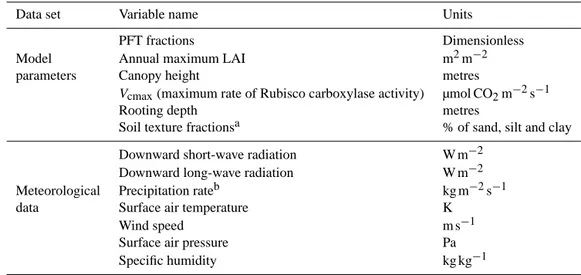
Table 1. Model parameters and meteorological variables that are altered between global and local model simulations.
Data set Variable name Units
PFT fractions Dimensionless
Model Annual maximum LAI m2m−2
parameters Canopy height metres
Vcmax(maximum rate of Rubisco carboxylase activity) µmol CO2m−2s−1
Rooting depth metres
Soil texture fractionsa % of sand, silt and clay
Downward short-wave radiation W m−2
Downward long-wave radiation W m−2
Meteorological Precipitation rateb kg m−2s−1
data Surface air temperature K
Wind speed m s−1
Surface air pressure Pa
Specific humidity kg kg−1
aThe soil texture fractions (%) are used to compute the soil hydraulic and thermal characteristics.
bAt some of the flux tower sites, the precipitation variable was separated into a rainfall rate (kg m−2s−1) and snowfall rate
(kg m−2s−1).
Predictions of the future uptake of atmospheric CO2by the
terrestrial biosphere are uncertain and this uncertainty comes from whether the terrestrial biosphere will continue to be a sink or source for CO2. The Coupled Climate–Carbon Cycle
Model Intercomparison Project (C4MIP) was the first major study to examine the coupling between climate change and the carbon cycle (Friedlingstein et al., 2006). One of its main conclusions was the reduced efficiency of the earth system, in particular the land carbon sink, to absorb increased an-thropogenic CO2. However, the magnitude of this effect
de-pended on the model used.
Land surface models (LSMs) are an important component of climate models and simulate the interaction between the atmosphere and terrestrial biosphere. They represent the sur-face energy and water balance, climate effect of snow and carbon fluxes (Pitman, 2003) and are considered the lower boundary condition for global climate models (GCMs) (Best et al., 2011). GCMs require the carbon, water and energy fluxes between the land surface and atmosphere to be speci-fied. Meteorological data, vegetation and soil characteristics are provided as inputs to LSMs, and using these, LSMs can predict fluxes, such as latent and sensible heat, upward long-wave radiation and net ecosystem exchange of CO2, which
is used to determine global atmospheric CO2concentrations.
Various LSMs have been designed over the last 40 years to calculate these fluxes (Dai et al., 2003).
The earliest GCMs to include a representation of the land surface based it on the simple “bucket” model. In this model, the soil is assumed to have a fixed water capacity (like a bucket) and at each land grid box and time step, the bucket is filled with precipitation and emptied by evaporation (Carson, 1982). The excess above its capacity is termed runoff. This model does not take vegetation or soil types into account. The
second generation of land surface schemes attempted to ex-plicitly represent the effects of vegetation in surface energy balance calculations and include the Biosphere-Atmosphere Transfer Scheme (BATS) (three soil layers and one vegeta-tion layer) (Dickinson, 1986) and the Simple Biosphere (SiB) Model (three soil layers and two vegetation layers) (Sell-ers et al., 1986). The current generation of models include the biological control of evapotranspiration with biochemi-cal models of leaf photosynthesis linked to the biophysics of stomatal conductance (Farquhar et al., 1980; Bonan, 2008), and can respond to changes in atmospheric CO2 in a more
realistic way.
evalu-ated, are used by different modelling groups to test model performance (Abramowitz, 2012; Luo et al., 2012). This has previously been carried out by Abramowitz et al. (2008) and Blyth et al. (2011).
Blyth et al. (2011) evaluated JULES at 10 FLUXNET sites, representing a range of biomes and climatic conditions, where model parameter values were taken as if the model was embedded in a GCM, in order to assess the model’s ability to predict observed water and carbon fluxes. We ex-tended this work by performing model simulations whereby model parameters (Table 1) were set to observe local site conditions and were then compared to those using global and satellite data. Local site conditions were those relevant to a particular flux tower site and were obtained from the re-search literature, communications with site Primary Investi-gator and the Ameriflux data archive. Global data referred to the model parameters taken from data sets used by the global operational version of JULES and meteorological data from global gridded data sets extracted for each flux tower grid box. The satellite data referred to LAI data from the MODer-ate resolution Imaging Spectroradiometer (MODIS) instru-ment, aboard NASA’s Earth Observing System (EOS) satel-lites, Terra and Aqua (http://modis.gsfc.nasa.gov).
In this study, we used 12 FLUXNET sites that cover a range of ecosystem types; temperate (6), boreal (2), mediterranean (2) and tropical (2) (Table 2), to investigate differences between using local, global and satellite-derived data sets when performing model simulations with JULES version 3.0 (Clark et al., 2011; Best et al., 2011). In particu-lar, we wished to address the following research questions:
– How well does JULES perform when using the best available local meteorological and parameter data sets? Can the model simulate interannual variability? – How well does JULES perform when using global data? – Of the global meteorological data sets used in this study,
which one compares best to FLUXNET data?
– Are improvements in simulated gross primary produc-tivity (GPP) observed when forcing JULES with daily satellite phenology compared to using the default phe-nology module?
2 Methods and model 2.1 Model description
The Joint UK Land Environment Simulator (JULES) is the land surface scheme of the UK Met Office Unified Model (UM) (current version 8.6), a family of models that includes the Hadley Centre Global Environmental Model (HadGEM) climate model (http://www.metoffice.gov.uk/ research/modelling-systems/unified-model). It has evolved from the Met Office Surface Exchange Scheme (MOSES)
(Cox et al., 1999). JULES is a mechanistic model and is able to model such processes as photosynthesis, evapotranspira-tion, soil and snow physics, and soil microbial activity (Blyth et al., 2011). Each model grid box is composed of nine dif-ferent surface types, five of which are vegetation, referred to as plant functional types (PFTs) (broadleaf trees, needleleaf trees, C3 (temperate) grass, C4 (tropical) grass and shrubs), and four non-vegetation types (urban, inland water, bare soil and land-ice). Each grid box can be made up of the first eight surface types or is land-ice. For single-point model simula-tions, as used in this study, each point is treated as a grid box with data such as surface type fractions, soil texture fractions and meteorological data used as input to the model.
The surface fluxes of CO2associated with photosynthesis
are computed on each time step for each PFT using a cou-pled photosynthesis-stomatal conductance model (Cox et al., 1998). These accumulated carbon fluxes are passed to TRIF-FID (Top-down Representation of Interactive Foliage and Flora Including Dynamics), JULES’ dynamic global veg-etation model and also its terrestrial carbon cycle compo-nent (Cox, 2001). TRIFFID updates the areal coverage, LAI and canopy height for each PFT on a longer time step (usu-ally every 10 days), based on the net carbon available to it and competition with other vegetation types (Cox, 2001). For these model simulations, vegetation competition was dis-abled, which meant that the PFT fractions for each site were prescribed and did not vary with time. If vegetation competi-tion was switched on during the spin-up process, this would have introduced error into the model simulations due to un-realistic vegetation fractions.
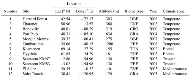
Table 2. Flux towers used in this study. The following biome types were used: deciduous broadleaf forest (DBF); evergreen needleleaf forest
(ENF); cropland (CRO); grassland (GRA); tundra (TUN); evergreen broadleaf forest (EBF).
Location
Number Site Lat [◦N] Long [◦E] Altitude (m) Biome type Year Climate zone
1 Harvard Forest 42.54 −72.17 303 DBF 2008 Temperate
2 Tharandt 50.96 13.57 380 ENF 2003 Temperate
3 Bondville 40.01 −88.29 219 CRO 2000 Temperate
4 Fort Peck 48.31 −105.10 634 GRA 2004 Temperate
5 Morgan Monroe 39.32 −86.41 275 DBF 2007 Temperate
6 Tumbarumba −35.66 148.15 1200 EBF 2008 Temperate
7 Kaamanen 69.14 27.29 155 TUN 2002 Boreal
8 Hyytiala 61.85 24.29 181 ENF 2003 Boreal
9 Santarem KM67 −2.86 −54.96 130 EBF 2003 Tropical
10 Santarem KM83 −3.02 −54.98 130 EBF 2001 Tropical
11 El Saler 39.35 −0.32 10 ENF 2003 Mediterranean
12 Vaira Ranch 38.41 −120.95 129 GRA 2005 Mediterranean
Table 3. Types of model simulations performed in this study.
Model Parameter Meteorological LAIb Phenologyc
simulationsa sets forcing
local-F local FLUXNET local Default
local local-WEIG local WFDEI-GPCC local Default
vs. global global-WEIG global WFDEI-GPCC global Default
data global-WEIC global WFDEI-CRU global Default
global-P global PRINCETON global Default
Satellite local-FNM local FLUXNET Site max. MODIS LAI Default phenology local-FM local FLUXNET Site max. MODIS LAI Daily forcing
aFor model simulation names, local and global refer to the parameter set and F, WEIG, WEIC and P refer to the meteorological forcing
data set used.
bFor LAI, local refers to the observed annual maximum LAI at each site and global refers to that obtained from the look-up tables used
by the global operational version of the model.
cDefault refers to the default phenology model used by JULES and daily forcing means that the default phenology has been switched
off and the model forced with daily MODIS LAI.
2.2 Experimental design
Offline single point simulations of GPP were performed at each of the 12 flux tower sites using various global and lo-cal data sets (Table 3). Correct simulation of GPP is impor-tant since errors in its calculation can propagate through the model and affect biomass and other flux calculations, such as net ecosystem exchange (NEE) (Schaefer et al., 2012). In JULES, NEE is not a model output and is calculated as total ecosystem respiration minus GPP. The correct representation of leaf level stomatal conductance has an influence on GPP and transpiration. Errors in GPP can also introduce errors into simulated latent and sensible heat fluxes. These study sites (Blyth et al., 2011; Abramowitz et al., 2008, Table 5) were chosen to validate model performance in carbon flux simulation since gap-filled meteorological data, local obser-vations of vegetation and soil characteristics and observed GPP fluxes were available.
One year model simulations were performed and span a range of years due to limited availability of local gap-filled meteorological data, observations of GPP fluxes and vegeta-tion characteristics (Table 2). Prior to performing the model simulations, the soil carbon pools at each site were brought to equilibrium using a 10 year spin-up by cycling 5 year aver-aged meteorological data (in equilibrium mode), followed by a 1000 year spin-up by cycling observed meteorological data (in dynamical mode). At Tumbarumba, Santarem Km67 and Santarem Km83, 3 year averaged meteorological data was used in the first part of the spin-up process due to limited data availability. More information on model spin-up can be found in Clark et al. (2011).
2.3 Data
runs using local data and 3-hourly data for simulations us-ing global data. For offline simulations, the model requires downward short-wave and long-wave radiation (W m−2),
rainfall and snowfall rate (kg m−2s−1), air temperature (K), wind speed (m s−1), surface pressure (Pa) and specific hu-midity (kg kg−1) (Table 1). Gap-filled meteorological forcing data at the local scale was obtained from the FLUXNET net-work and data at the global scale was obtained from two grid-ded data sets: WFDEI (Weedon et al., 2014, 2011) and that developed by Sheffield et al. (2006) (referred to as PRINCE-TON).
Vegetation and soil parameters (Table 1) were adjusted to local or global values depending on the model simulations (Table 3) performed at the 12 flux tower sites. Local vegeta-tion (Tables 5, 6) and soil parameters (not shown) were ob-tained from the research literature, communications with site Primary Investigator and the Ameriflux data archive. Global vegetation (Tables 5, 6) and soil parameters (not shown) were taken from data sets used in the global operational version of JULES as used in the Hadley Centre Global Environmen-tal Model (HadGEM) climate model. These data sets include the Global Land Cover Characterization (version 2) database (http://edc2.usgs.gov/glcc/glcc.php) (PFT fractions), and the Harmonized World Soil Database (version 1.2) (Nachter-gaele et al., 2012) (soil texture fractions).
There are several global LAI data sets available, such as ECOCLIMAP (1992) (Masson et al., 2003), CYCLOPES (1997–2007) (Baret et al., 2007), GLOBCARBON (1998– 2003) (Deng et al., 2006), MOD15 (2000–present) (Yang et al., 2006) and MISR LAI (2000–present) (Diner et al., 2008; Hu et al., 2007). For the majority of sites used in this study, gap-filled meteorological data and GPP flux observa-tions are only available for the 2000s and therefore, a global data set of satellite LAI was required that covered this period. We used the MODIS LAI product because it is a high spatial and temporal resolution data set with global coverage. 2.3.1 Forcing data
FLUXNET, a “network of regional networks”, is a global network of micrometeorological tower sites that measure the exchange of carbon dioxide, water vapour and energy be-tween the biosphere and atmosphere across a range of biomes and timescales (Baldocchi et al., 2001). Data and site infor-mation are available online at: http://www.fluxnet.ornl.gov/. Over 500 tower sites are located worldwide on five conti-nents and are used to study a range of vegetation types, such as temperate conifer and broadleaved (deciduous and ever-green) forests, tropical and boreal forests, crops, grasslands, wetlands, and tundra (Baldocchi et al., 2001).
The WATCH Forcing Data (WFD) (1901–2001) was cre-ated in the framework of the Water and Global Change (WATCH) project (http://www.eu-watch.org/), which sought to assess the terrestrial water cycle using land surface mod-els and general hydrological modmod-els. WFD was derived using
the 40 years ECMWF Re-Analysis (ERA-40) for 1958–2001 and data for 1901–1957 was obtained using random years ex-tracted from the ERA-40 data (Weedon et al., 2011). WFD was extended by applying the WFD methodology to the ERA-Interim data for the 1979–2009 period (WFDEI) (Wee-don et al., 2014). Within WFD and WFDEI, there are two precipitation products: the first corrected using the Climate Research Unit at the University of East Anglia (CRU) ob-servations; and the second using Global Precipitation Clima-tology Centre (GPCC) observations. The WFDEI data sets incorporating the GPCC- and CRU-corrected precipitation products are referred to as WFDEI-GPCC and WFDEI-CRU, respectively. WFDEI is only available for land points includ-ing Antarctica, and consists of 3-hourly, regularly (latitude– longitude) gridded data at half-degree (0.5◦×0.5◦) resolu-tion. This resolution produces a global grid of 360×720 grid cells and is equivalent to a surface resolution of about 56 km×56 km at the Equator and 56 km×32 km at 55◦N
(temperate regions).
The Sheffield et al. (2006) data set (PRINCETON) is a global 60-year meteorological data set for driving land sur-face models developed by the Land Sursur-face Hydrology Re-search Group at Princeton University. PRINCETON is only available for land points (excluding Antarctica), and con-sists of 3-hourly, 1◦ resolution, meteorological data for the 1948–2008 period. This data set has a resolution half that of WFDEI with a global grid of 180×360 grid cells and is equivalent to a surface resolution of about 111 km×111 km at the Equator and 111 km×64 km at 55◦N. The resolution (both spatial and temporal) of the meteorological data can affect the output of land surface and atmospheric chemistry models (Pugh et al., 2013; Ashworth et al., 2010; Ito et al., 2009; Guenther et al., 2006) and may introduce a systematic bias.
2.3.2 Observational data
Local observations of GPP were obtained from the FLUXNET network. Flux tower sites use the eddy covari-ance method to measure net ecosystem exchange (NEE), which is defined as the net flux of CO2, and is separated into
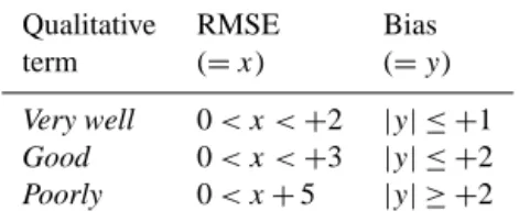
Table 4. Definition of qualitative terms used to describe JULES’
ability to simulate GPP when compared to observed FLUXNET GPP. Both RMSE and Bias have units of g C m−2day−1. Starting at “Very well”, the term associated with the first condition satisfied is used to describe model performance.
Qualitative RMSE Bias term (=x) (=y)
Very well 0< x <+2 |y| ≤ +1
Good 0< x <+3 |y| ≤ +2
Poorly 0< x+5 |y| ≥ +2
2.3.3 Ecological and soil data
The Global Land Cover Characterization (version 2) database, generated by the US Geological Survey, the Uni-versity of Nebraska-Lincoln, and the European Commis-sion’s Joint Research Centre, is a 1 km resolution global land cover data set for use in environmental and modelling re-search (Loveland et al., 2000). Land cover is classified into 17 categories using the International Geosphere–Biosphere Programme (IGBP) scheme. The land cover category for each of the flux tower sites was extracted from the GLCC database (IGBP code in Table 5). These IGBP codes are then used to derive the annual maximum LAI and canopy height for each PFT from the look-up tables used in the global oper-ational version of JULES. Further information on how these variables are derived can be found in Appendix A.
Global soil texture fractions (% of sand, silt and clay) for each of the 12 FLUXNET sites (not shown here) were extracted from the Harmonized World Soil Database (ver-sion 1.2) (HWSD) (Nachtergaele et al., 2012). The equations used to compute soil hydraulic and thermal characteristics were taken from the Unified Model Documentation Paper No. 70 (Jones, 2007). Note that the equations in Jones (2007) apply only to mineral soils, as organic soils behave differ-ently (Gornall et al., 2007). In this study, the soils are clas-sified as mineral at all 12 sites. Since the HWSD contains soil textures for two soil depths (0–30 and 30–100 cm) and JULES contains four soil layers (thicknesses of 0.1, 0.25, 0.65 and 2.0), the 0–30 cm soil textures were assigned to the top two model soil layers (thicknesses 0.1 and 0.25 m, re-spectively), and the 30–100 cm textures were assigned to the bottom two layers (thicknesses 0.65 and 2.0 m, respectively). The local soil textures are provided as site averages and therefore, each model soil layer (four in total) is assigned the same set of soil textures.
2.3.4 MODIS LAI products
The MODIS LAI product, computed from MODIS spectral reflectances, provides continuous and consistent LAI cov-erage for the entire global land surface at 1 km resolution (Yang et al., 2006). Some gaps and noise in the data are
possible due to the presence of cloudiness, seasonal snow cover and instrument problems, and this can limit the useful-ness of the product (Gao et al., 2008; Lawrence and Chase, 2007). In this study, we use the MODIS Land Product Sub-sets, created by the Oak Ridge National Laboratory Dis-tributed Active Archive Center (ORNL DAAC), which pro-vide summaries of selected MODIS Land Products for use in model validation and field site characterisation and in-clude data for more than 1000 field sites and flux towers (http://daac.ornl.gov/MODIS/).
The MODIS Land Product Subsets (ASCII format) con-tain LAI data for a 7 km×7 km grid of 49 pixels, with each pixel representing the 1 km×1 km scale, at 8-day composite intervals. The average of the 3×3 pixel grid box centred on the flux tower is taken to be that day’s LAI value. Only pixel values with an even quality control (QC) flag was used for the averaging and this produced a time-series of 8-day ob-servations at each of the sites. Missing data were dealt with by using the previous good value in the time-series. The ex-ception to this was Bondville, where missing data occurred in January 2000, since MODIS only started recording data in February 2000 (this year was used due to limited data avail-ability at the site). To gap-fill the missing data, an 11-year av-erage was computed and the missing data replaced with the average for January 2000. Finally, each time-series of 8-day composite values was linearly interpolated to obtain a daily LAI time-series.
2.4 Outline of experiments
This section describes the model simulations performed in the study. In the model simulation names, local and global refer to the parameter set and F, WEIG, WEIC and P refer to the meteorological forcing data set used (Table 3). Vegetation competition has been switched off for all model simulations.
2.4.1 Effect of local data on simulated GPP
Using JULES3.0, we compared model simulations using lo-cal parameter and meteorologilo-cal data sets (lolo-cal-F; Table 3) to observations of GPP from the FLUXNET network. For this set of model simulations, the default phenology model (used to update LAI) and TRIFFID were used.
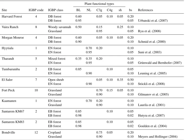
Table 5. Vegetation (PFT) and non-vegetation land cover type (BL: broadleaf tree, NL: needleleaf tree, C3g: C3 grass, C4g: C4 grass, sh:
shrubs, bs: bare soil) fractions at the 12 FLUXNET sites. For each site, the first row refers to global data and the second refers to local.
Plant functional types
Site IGBP code IGBP class BL NL C3g C4g sh bs References
Harvard Forest 4 DB forest 0.60 0.05 0.10 0.05 0.20
DB forest 0.95 0.05 Urbanski et al. (2007)
Vaira Ranch 8 Woody savannah 0.50 0.15 0.25 0.10
Grassland 0.95 0.05 Ryu et al. (2008)
Morgan Monroe 4 DB forest 0.60 0.05 0.10 0.05 0.20
DB forest 0.90 0.10 Schmid et al. (2000)
Hyytiala 1 EN forest 0.70 0.20 0.10
EN forest 0.95 0.05 Suni et al. (2003)
Tharandt 5 Mixed forest 0.35 0.35 0.20 0.10
EN forest 0.95 0.05 Grünwald and Bernhofer (2007)
Tumbarumba 2 EB forest 0.85 0.10 0.05
EN forest 0.90 0.10 Leuning et al. (2005)
El Saler 7 Open shrub 0.05 0.10 0.35 0.50
EN forest 0.90 0.10 Stöckli et al. (2008)
Fort Peck 10 Grassland 0.70 0.15 0.05 0.10
Grassland 0.90 0.10 Gilmanov et al. (2005)
Kaamanen 1 EN forest 0.70 0.20 0.10
Grassland 0.90 0.10 Laurila et al. (2001)
Santarem KM67 2 EB forest 0.85 0.10 0.05
EB forest 0.98 0.02 Hutyra et al. (2007)
Santarem KM83 2 EB forest 0.85 0.10 0.05
EB forest 0.98 0.02 Goulden et al. (2004)
Bondville 12 Cropland 0.75 0.05 0.20
Grassland 0.90 0.10 Meyers and Hollinger (2004)
2.4.2 Effect of global data on simulated GPP
Using JULES3.0, we compared model simulations using pa-rameter sets from the HadGEM model and global meteoro-logical data (global-WEIG, global-WEIC and global-P; Ta-ble 3) to observations of GPP from the FLUXNET network. In addition to this, we quantified how much error is intro-duced into model simulations (using local model parameters) when using global (WFDEI-GPCC) instead of local meteo-rological data (local-WEIG and local-F in Table 3). In these model simulations, the default phenology model and TRIF-FID were used.
2.4.3 Comparison of global to local meteorological data
The WFDEI-GPCC, WFDEI-CRU and PRINCETON data sets were compared to FLUXNET to find out which one more closely captures the local meteorological conditions.
2.4.4 Daily satellite phenology
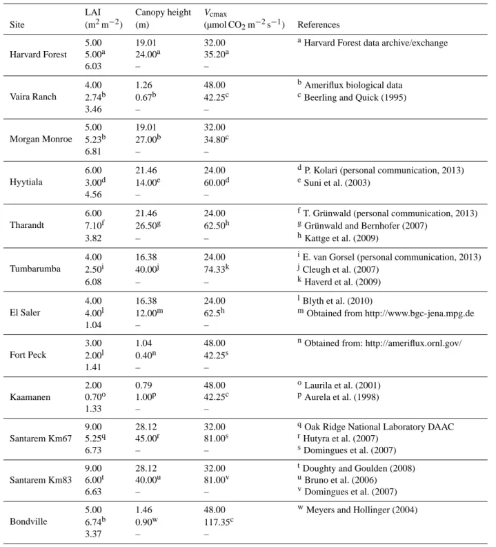
Table 6. Local and global biophysical parameters (site annual maximum LAI, canopy height andVcmax) at the 12 FLUXNET sites. For each
site, the first row refers to global data, the second refers to local and the third refers to satellite. Online data was accessed in April 2013.
LAI Canopy height Vcmax
Site (m2m−2) (m) (µmol CO2m−2s−1) References
Harvard Forest
5.00 19.01 32.00 aHarvard Forest data archive/exchange 5.00a 24.00a 35.20a
6.03 – –
Vaira Ranch
4.00 1.26 48.00 bAmeriflux biological data
2.74b 0.67b 42.25c cBeerling and Quick (1995)
3.46 – –
Morgan Monroe
5.00 19.01 32.00
5.23b 27.00b 34.80c
6.81 – –
Hyytiala
6.00 21.46 24.00 dP. Kolari (personal communication, 2013) 3.00d 14.00e 60.00d eSuni et al. (2003)
4.56 – –
Tharandt
6.00 21.46 24.00 fT. Grünwald (personal communication, 2013) 7.10f 26.50g 62.50h gGrünwald and Bernhofer (2007)
3.82 – – hKattge et al. (2009)
Tumbarumba
4.00 16.38 24.00 iE. van Gorsel (personal communication, 2013) 2.50i 40.00j 74.33k jCleugh et al. (2007)
6.08 – – kHaverd et al. (2009)
El Saler
4.00 16.38 24.00 lBlyth et al. (2010)
4.00l 12.00m 62.5h mObtained from http://www.bgc-jena.mpg.de
1.04 – –
Fort Peck
3.00 1.04 48.00 nObtained from: http://ameriflux.ornl.gov/ 2.00l 0.40n 42.25s
1.41 – –
Kaamanen
2.00 0.79 48.00 oLaurila et al. (2001)
0.70o 1.00p 42.25c pAurela et al. (1998)
1.33 – –
Santarem Km67
9.00 28.12 32.00 qOak Ridge National Laboratory DAAC
5.25q 45.00r 81.00s rHutyra et al. (2007)
6.73 – – sDomingues et al. (2007)
Santarem Km83
9.00 28.12 32.00 tDoughty and Goulden (2008)
6.00t 40.00u 81.00v uBruno et al. (2006)
6.63 – – vDomingues et al. (2007)
Bondville
5.00 1.46 48.00 wMeyers and Hollinger (2004)
6.74b 0.90w 117.35c
3.37 – –
2.5 Model analyses
To quantify differences between output from the various model simulations and observations, we used root mean squared error (RMSE) (Eq. 1), which is a measure of the av-erage error of the simulations, and bias (Eq. 2), which is the average difference between model and observations (a mea-sure of under- or overprediction) with the absolute (Eq. 3)
and percentage differences (Eq. 4):
RMSE=
s Pt=n
t=1(xt−xo, t)2
n , (1)
Bias=
Pt=n
t=1xt−Ptt==n1xo, t
n . (2)
xtandxo, tare model and observed daily GPP fluxes,
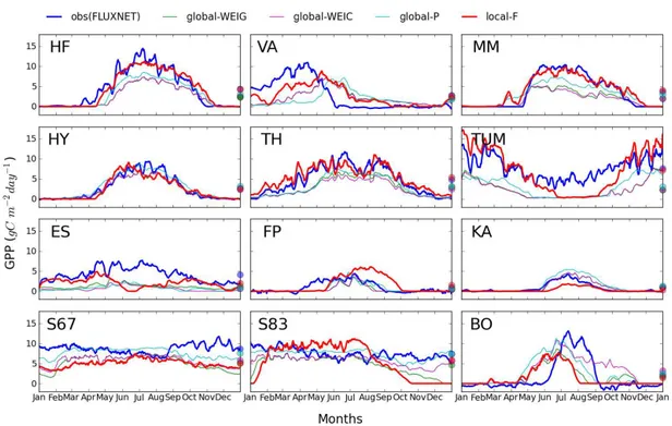
aver-Figure 1. Seasonal cycle of model-predicted (local-F, global-WEIG, global-WEIC and global-P in Table 3) and observed GPP fluxes,
smoothed with a 7-day moving average window, at the 12 FLUXNET sites (HF: Harvard Forest; VA: Vaira Ranch; MM: Morgan Monroe; HY: Hyytiala; TH: Tharandt; TUM: Tumbarumba: ES: El Saler; FP: Fort Peck; KA: Kaamanen; S67: Santarem Km67; S83: Santarem Km83; BO: Bondville). Model simulation years are given in Table 2. The thick lines refer to FLUXNET observations (blue) and simulated GPP from local-F model simulations (red). Annual averages for model simulations and observations are plotted as thick dots on the right of each plot in the same colours.
age since we are interested in the long-term average and not daily variability.nis the number of paired values (number of days in year). The absolute difference (1GPP) between the model and observations is the absolute value of the difference in total annual GPP for each and the percentage difference (1%) is the absolute difference divided by the observed total annual GPP:
1GPP= |XGPPobs−
X
GPPmodel|, (3)
1%=P1GPP GPPobs
×100. (4)
In order to describe JULES’ ability to reproduce simulated GPP, a simple, but subjective, ranking system using qualita-tive terms (Very well, Good and Poorly) was devised based on RMSE and bias (Table 4, Fig. 2a). These ranges were used as interannual variability was about±1 g C m−2day−1 in both RMSE and bias (Sect. 3.1).
3 Results
3.1 Effect of local data on simulated GPP
When driven with local meteorological and parameter data sets (local-F; Fig. 1), JULES has a negative bias with total annual GPP underestimated by 16 % (3049 g C m−2year−1;
Table 7) across all sites compared to observations. By us-ing local data, JULES performs very well (see Fig. 2a and Table 4 for definition of qualitative terms used to de-scribe model performance) at the temperate forest sites, Harvard Forest, Morgan Monroe, Hyytiala and Tharandt, where RMSEs range from 1.1–1.4 g C m−2day−1, biases
from−0.2 to+0.3 g C m−2day−1(Fig. 2a) and absolute
dif-ferences from 40–211 g C m−2year−1 (Table 7) and good
at Vaira Ranch with an RMSE of 2.78 g C m−2day−1, bias of −0.19 g C m−2day−1 and absolute difference of 71 g C m−2year−1. The model performs poorly at Tum-barumba, El Saler, Bondville and the tropical sites, Santarem Km67 and Santarem Km83, with RMSEs ranging from 1.8– 4.1 g C m−2day−1, biases from−3.7 to−0.2 g C m−2day−1 and absolute differences from 71–1340 g C m−2year−1.
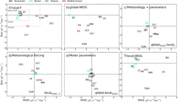
Figure 2. Comparison of modelled and observed GPP using bias and RMSE at the 12 FLUXNET sites (HF: Harvard Forest; VA: Vaira Ranch;
MM: Morgan Monroe; HY: Hyytiala; TH: Tharandt; TUM: Tumbarumba; ES: El Saler; FP: Fort Peck; KA: Kaamanen; S67: Santarem Km67; S83: Santarem Km83; BO: Bondville) for three sets of model simulations: (a) local-F; (b) global-WEIG; and (f) local-WEIG (Table 3). (c) displays the differences between bias and RMSE for global-WEIG and local-F model simulations; (d) differences between local-WEIG and local-F model simulations; and (e) differences between global-WEIG and local-WEIG model simulations. Marked on (c), (d) and (e) next to the figure letter are how the sets of model simulations differ. The site labels are coloured according to their climate zone (Table 2). The dashed lines on (a) show the regions defined by the qualitative terms (Table 4) used to describe model performance.
Table 7. Absolute and percentage differences between model simulated and observed (FLUXNET) total annual GPP (gC m−2year−1) at the 12 flux tower sites.P
GPPobsis the observed total annual GPP,1GPP is the absolute difference (Eq. 3) between the model and observed
total annual GPP, and1% is the percentage difference (Eq. 4) between the model and observed total annual GPP. Values highlighted in bold mean that the difference is negative (i.e.P
GPPobs<PGPPmodel). The total value for each of the model simulations was computed using
the differences and not the absolute differences.
FLUXNET local-F local-WEIG global-WEIG global-WEIC global-P
Site P
GPPobs 1GPP 1% 1GPP 1% 1GPP 1% 1GPP 1% 1GPP 1%
Harvard Forest 1621 40 2 567 35 716 44 711 44 486 30
Vaira Ranch 1047 71 7 592 57 235 22 259 25 369 35
Morgan Monroe 1385 94 7 639 46 616 44 661 48 256 18
Hyytiala 997 68 7 73 7 135 14 120 12 144 14
Tharandt 1754 211 12 306 17 687 39 819 47 590 34
Tumbarumba 2806 197 7 1710 61 1951 70 1984 71 1690 60
El Saler 1512 760 50 499 33 1073 71 1276 84 1234 82
Fort Peck 367 194 53 229 62 213 58 200 54 105 29
Kaamanen 368 249 68 273 74 8 2 5 1 124 34
Santarem Km67 3171 1340 42 451 14 1245 39 1075 34 392 12
Santarem Km83 2724 583 21 202 7 1033 38 644 24 40 1
Bondville 766 240 31 200 26 131 17 406 53 177 23
Total 18 518 3049 4325 8043 7348 4717
GPP being underestimated by 42 % (1340 g C m−2year−1) and 21 % (583 g C m−2year−1), respectively (Table 7).
JULES can simulate interannual variability when using lo-cal data with average RMSEs across all six sites for all years
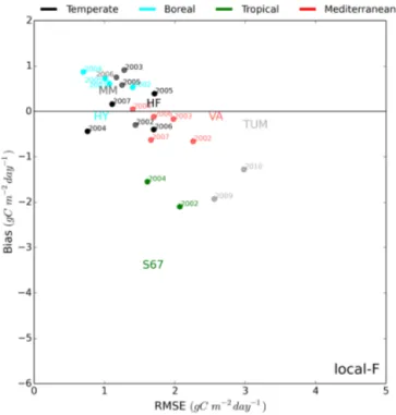
Figure 3. Multi-year comparison of modelled and observed GPP
using bias and RMSE at six FLUXNET sites (HF: Harvard For-est; VA: Vaira Ranch; MM: Morgan Monroe; HY: Hyytiala; TUM: Tumbarumba; S67: Santarem Km67) for model simulations using local parameter and meteorological data (local-F). The site labels are coloured according to their climate zone (Table 2) and repre-sent data from model simulations performed for the year specified in Table 2, with results from other years plotted using the model simulation year and labels coloured the same as the original site label.
and Morgan Monroe) and Vaira Ranch with RMSEs rang-ing from +1 to +3 g C m−2day−1 and biases from +1 to
−1 g C m−2day−1. As observed with the single-site model simulations, the model fails to capture interannual variability at Santarem Km67 and Tumbarumba (Fig. 3).
Overall, JULES performs very well with the use of local data (meteorological and parameter data sets) with negative biases observed at the tropical sites and the Southern Hemi-sphere site, Tumbarumba, with the same trend also observed when the model simulates interannual variability.
3.2 Effect of global data on simulated GPP
By replacing the local data with global parameter and meteorological data, JULES had a much greater nega-tive bias with total annual GPP underestimated by 30 % (6703 g C m−2year−1; Table 7) on average across all sites compared to observations (global-WEIG, global-WEIC and global-P; Fig. 1). This is also shown in the annual average GPP, which has been plotted for each of the model simula-tions and observasimula-tions at the 12 sites (Fig. 1) and the percent-age differences (Table 7), which are, in general, larger for simulations using global data than for those using local. This
trend occurs at all sites, with the exception of the wetland site, Kaamanen, and Santarem Km83, where modelled total annual GPP (2684 g C m−2year−1 and 492 g C m−2year−1,
respectively) is overestimated (global-P; Table 7) compared to model runs using only local data (2141 g C m−2year−1and 119 g C m−2year−1, respectively; Table 7).
As well as quantifying differences in model simulations using either local or global data, it is useful to know how global meteorological data affects local model runs. Global meteorological data can be used in place of FLUXNET data in order to drive JULES (local-WEIG; Table 3). This is im-portant for ecological research sites where there is limited or no local meteorological data available. Using the WFDEI-GPCC meteorological data set (local-WEIG; Table 3) to force the model increases the negative bias of model simu-lations using only local data (Fig. 2f), with a 7 % reduction in simulated total annual GPP (15 469 g C m−2year−1 for
local-F reduced to 14 193 g C m−2year−1 for local-WEIG;
Table 7).
Forcing the model with WFDEI-GPCC (local-WEIG) re-sults in decreases in model performance (increases in bias and RMSE) at the majority of sites. The tropical sites, Santarem Km67 and Santarem Km83, are two exceptions and show a noticeable improvement in modelled yearly GPP (66 and 61 % reduction of bias, respectively) and changes to modelled seasonal cycle (25 % increase and 65 % reduc-tion of RMSE, respectively). However, at some sites, such as Tharandt, Kaamanen and Hyytiala, forcing JULES with global meteorological data has not introduced large negative biases into GPP predictions (Table 7), with RMSEs ranging from 1.1–1.3 g C m−2year−1(Fig. 2f).
In general, we found the meteorological data had a greater impact on modelled GPP fluxes than model parameters. Larger differences exist between local-WEIG and local-F (localWEIG-F; Fig. 2d), which differ only in the atmospheric
forcings data set used, compared to between global-WEIG and local-WEIG (global−localWEIG; Fig. 2e), which differ
only in the model parameter sets used.
The ability of JULES to capture yearly GPP (bias) and the seasonal cycle (RMSE) is affected at the majority of sites when using global meteorological data (Fig. 2d), with improvements observed at Santarem Km67 and Santarem Km83. However, model parameters were found to affect bias at all 12 sites (Fig. 2e) with the tropical sites being the most influenced. With the exception of Tumbarumba, biases associated with meteorological data compensate for those associated with model parameters at the tropical sites (globalWEIG−localF; Fig. 2c).
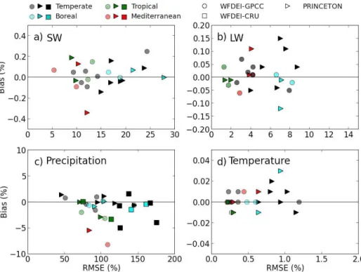
Figure 4. Bias and RMSE, expressed as percentages of daily average, when comparing global (WFDEI-GPCC (circles), WFDEI-CRU
(squares) and PRINCETON (triangles)) to local meteorological data for four meteorological variables: (a) downward short-wave radiation (SW); (b) downward long-wave radiation (LW); (c) precipitation; and (d) surface air temperature, at the 12 FLUXNET sites (HF: Harvard Forest; VA: Vaira Ranch; MM: Morgan Monroe; HY: Hyytiala; TH: Tharandt; TUM: Tumbarumba; ES: El Saler; FP: Fort Peck; KA: Kaamanen; S67: Santarem Km67; S83: Santarem Km83; BO: Bondville). The site labels are coloured according to their climate zone (Table 2). Note that before computing bias and RMSE, the meteorological data was normalised against the annual mean for each site.
improves model performance. We found the meteorological data to have a greater impact on GPP fluxes than model pa-rameters.
3.3 Global vs. local meteorological data
As well as quantifying the error introduced into model sim-ulations by using global meteorological data instead of cal, we also compared the global meteorological data to lo-cal data. Only the downward short-wave and long-wave ra-diation fluxes, precipitation and surface air temperature vari-ables have been compared to FLUXNET values, since these variables play the most influential role of the meteorologi-cal forcings in canopy photosynthesis and light propagation in JULES (Alton et al., 2007). In order to compare the me-teorological data sets, the data was normalised against the annual mean for each site before computing the RMSE and bias.
Of the two global meteorological data sets used in this study, the WFDEI data set compares best to FLUXNET (lower RMSEs and biases than PRINCETON) at the major-ity of sites (Fig. 4). Surface air temperatures compare best to local meteorological measurements with average RMSEs of 0.4 and 0.7 % (7 day filtered RMSE expressed as per-centages of the annual mean value) (1.5 and 2.4 K) across all sites for the WFDEI and PRINCETON data sets,
respec-tively (Fig. 4d), followed by the downward short-wave ra-diation fluxes with average RMSEs of 13 and 17 % (27.0 and 33.2 W m−2) for WFDEI and PRINCETON, respectively
(Fig. 4a), and downward long-wave radiation fluxes with average RMSEs of 4 and 5 % (18.9 and 25.0 W m−2) for WFDEI and PRINCETON, respectively (Fig. 4b). Precipita-tion data from global data sets differ most from local values with RMSEs of 112–178 % (2.7–4.4 mm day−1) for WFDEI-GPCC, WFDEI-CRU and PRINCETON, respectively, which may be due to how the precipitation products of each global data set is corrected (Weedon et al., 2011; Sheffield et al., 2006).
al-though differences in the data sets may be more important when JULES is run globally.
Even though WFDEI compares better to the local me-teorological data than PRINCETON, we found that when JULES is forced with the PRINCETON data set, improve-ments in GPP predictions were observed at Santarem Km67 and Santarem Km83 (Fig. 1). We observed that at the tropical sites, the meteorological forcings were the primary driver of productivity for model simulations using global data and that biases associated with the global meteorological data com-pensated for incorrect parameter values.
By swapping local meteorological data with global me-teorological data (PRINCETON) for model simulations us-ing local data (local-F), it was found that the positive bias associated with global surface air temperature (PRINCE-TON) at Santarem Km83 is the primary cause of improved model performance (39 % reduction in RMSE) when us-ing global data and by forcus-ing JULES with the PRINCE-TON data set and using the lower global Vcmax value
(Ta-ble 6), the model was a(Ta-ble to reproduce the seasonal cy-cle very well (RMSE of 1.26 g C m−2day−1). At Santarem Km67, we found the downward long-wave radiation to be the main reason for the improved seasonal cycle (35 % re-duction in RMSE) and by using the PRINCETON data set and global Vcmax value (Table 6), model performance was
improved (RMSE of 2.12 g C m−2day−1).
Compensation between meteorological data and model pa-rameters also occurs at Hyytiala, where the model performs very well with global meteorological and parameter data sets (Fig. 1). The global downward short-wave radiation is larger than its locally measured value and this offsets the low global Vcmaxvalue at this site (Table 6, Fig. 6b).
Overall, we found the WFDEI data set compares bet-ter than PRINCETON to FLUXNET and of the four mete-orological variables examined, the radiation fluxes (down-ward short-wave and long-wave) and surface air tempera-tures compare very well to local values. Within the WFDEI data set, the two precipitation products (WFDEI-GPCC and WFDEI-CRU) compare equally well to FLUXNET precip-itation. Improvements were observed at the tropical sites when JULES is forced with PRINCETON and this is due to biases associated with the meteorological data.
3.4 Forcing JULES with daily satellite phenology The performance of LSMs depend on how well the seasonal variation of LAI is represented, since GPP is strongly influ-enced by the timing of budburst and leaf senescence (Liu et al., 2008). In JULES, LAI is essential for the calculation of plant canopy photosynthesis and is updated daily in response to temperature. We test the JULES phenology model by com-paring model predictions of GPP when JULES uses its de-fault phenology model with those in which JULES uses lo-cal data with the annual maximum LAI set to be the MODIS annual maximum LAI (local-FNM), and with those in which
the model uses local data and is forced with daily MODIS LAI (local-FM).
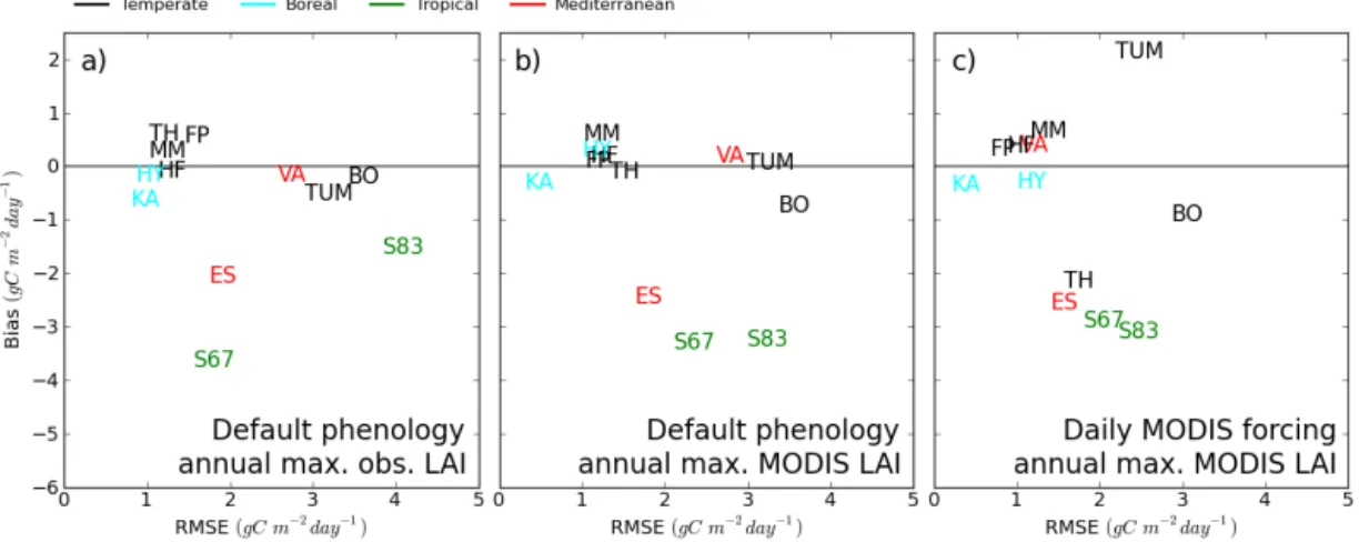
Forcing JULES with daily satellite LAI (local-FM) results in either small improvements (average reduction in RMSE by 0.2 g C m−2day−1) or none at all at the 12 flux tower sites (Fig. 5c). An average RMSE of 2.2 g C m−2day−1across all sites is observed when the model is forced with daily MODIS LAI (local-FM), which is less than that for model simula-tions using no MODIS information (local-F; average RMSE of 2.4 g C m−2day−1) and those which use the annual maxi-mum MODIS LAI as the annual maximaxi-mum LAI at each site (local-FNM; average RMSE of 2.39 g C m−2day−1).
By using MODIS data, there is only a small reduction (8 and 0.04 % for local-FM and local-FNM, respectively) in av-erage RMSE when simulating GPP compared to model runs that do not use it. Of the 12 sites, only seven (Harvard Forest, Vaira Ranch, Hyytiala, Tharandt, Tumbarumba, Kaamanen and Santarem Km67) show improved model performance when either being forced with daily MODIS LAI (Fig. 5c) or using the annual maximum MODIS LAI as the model an-nual maximum LAI (Fig. 5b). At these seven sites, simulated yearly GPP increases in total by 21 %. At the remaining sites, JULES performs better using the default phenology module (Fig. 5a).
Of the seven sites where JULES’ performance improved using MODIS data, forcing JULES with daily satellite phe-nology (local-FM) only resulted in improved model perfor-mance at Santarem Km67 (Fig. 5c) and at the remaining six sites, using the default phenology with the annual maximum MODIS LAI set to be the annual maximum LAI (Fig. 5b), JULES’ performance improved. Even with the addition of MODIS data, the model still performed poorly at Bondville, with only a slight improvement in predicted GPP (1 and 15 % reduction of RMSE for local-FM and local-FNM, re-spectively) compared to using only local data (RMSE of 3.66 g C m−2day−1).
The sites which display the largest improvements in sim-ulated GPP, when forced with MODIS LAI, are those which have low LAI values (54 and 24 % reduction in RMSE at Vaira Ranch and Fort Peck, respectively) (Fig. 5c). Small im-provements were also observed at the tropical sites (13 and 14 % reduction in RMSE at Santarem Km67 and Santarem Km83, respectively). At some sites, using MODIS data had no effect on model results (El Saler) and in some cases, the model performed worse (Tumbarumba).
The total annual simulated GPP for model runs us-ing MODIS data (15, 334 and 15, 227 g C m−2year−1, for
Figure 5. Comparison of modelled and observed GPP using bias and RMSE (computed using anomalies) at the 12 FLUXNET sites (HF:
Harvard Forest; VA: Vaira Ranch; MM: Morgan Monroe; HY: Hyytiala; TH: Tharandt; TUM: Tumbarumba; ES: El Saler; FP: Fort Peck; KA: Kaamanen; S67: Santarem Km67; S83: Santarem Km83; BO: Bondville) for three sets of model simulations: (a) default phenology model with locally observed annual maximum LAI (data values used same as in Fig. 2a (local-F)); (b) default phenology model with annual maximum MODIS LAI (model simulations local-FNM); and (c) daily MODIS forced model simulations with annual maximum MODIS LAI (model simulations local-FM). The site labels are coloured according to their climate zone (Table 2).
data and vegetation parameters, such asVcmax, may have a
greater impact on predicted GPP than LAI.
Overall, when JULES is forced with daily MODIS LAI small improvements (8 % reduction in average RMSE; local-FM) in predicted GPP are observed at a number of sites, though there exists a negative bias associated with using MODIS data. By setting the annual maximum MODIS LAI to be the annual maximum LAI at each site, the model per-forms equally well (0.04 % reduction in average RMSE; local-FNM) to local model simulations. We also observed improvements in simulated GPP at sites with low LAI val-ues, such as grasslands, when JULES is forced with daily LAI.
4 Discussion
4.1 How well does JULES perform when using the best available local meteorological and parameter data sets compared to those using global data?
At more than half of the sites, JULES performs very well when using local meteorological and parameter data sets with a negative bias observed for the remaining sites (Fig. 2a). At the six sites where multi-year model simulations were performed, interannual variability is captured by the model using local data with the exception of Santarem Km67 and Tumbarumba. This trend is also observed with the single-year runs.
The use of global parameter and meteorological data sets introduces a negative bias into GPP simulations at all sites with the exception of the mediterranean site, El Saler, and the tropical sites (Fig. 2b). Using local parameter and global me-teorological data to drive JULES (local-WEIG) increases the
negative bias of local model simulations (local-F) (Fig. 2f). We observed decreases in model performance at the ma-jority of sites, with the exceptions being the tropical sites (Santarem Km67/Km83). At some sites, such as Hyytiala and Kaamanen, using global meteorological data produced similar results (Fig. 2a, f) to using FLUXNET data.
Our results compare well with the evaluation of JULES by Blyth et al. (2011), where parameters were obtained as though the model was embedded in a GCM. Differences be-tween the two studies include different model versions and global meteorological data sets used. Comparing our results with Fig. 3 of Blyth et al. (2011), we also found simulated photosynthesis to be underestimated for the temperate forests (Harvard Forest, Tharandt and Morgan Monroe), grasslands (Fort Peck), mediterranean sites (El Saler) and the tropical forests (Santarem Km67), and overestimated for the wetlands (Kaamanen). We observed that the use of local observations of site characteristics, such as PFT fractions and vegetation properties, lead to improvements in model performance at more than half of the sites (Fig. 2a), though errors still exist with percentage differences ranging from 2–12 %.
Differences between global and local data include PFT fractions (Table 5), soil texture fractions, vegetation parame-ters (Table 6) and meteorological data. At some sites, such as Bondville and Santarem Km67/Km83, the global and local values for LAI andVcmaxwere markedly different (Fig. 6),
though for the majority of sites, global and local LAI val-ues were quite close (Fig. 6a), whereas globalVcmaxvalues
Figure 6. Comparison of (a) global, MODIS (site annual maximum) and local leaf area index (LAI) and (b) global and local maximum
rate of Rubisco carboxylase activity (Vcmax) at the 12 FLUXNET sites (HF: Harvard Forest; VA: Vaira Ranch; MM: Morgan Monroe; HY:
Hyytiala; TH: Tharandt; TUM: Tumbarumba; ES: El Saler; FP: Fort Peck; KA: Kaamanen; S67: Santarem Km67; S83: Santarem Km83; BO: Bondville). The LAI data displayed for each study site refer to the annual maximum LAI of the dominant PFT. The site labels are coloured according to their climate zone (Table 2) and in (a), the lighter shades are the MODIS data. The dashed grey lines represent LAI andVcmax,
where global, MODIS and local values match, with overestimated global and MODIS values above the dashed line and underestimated values below it.
In general, we found the meteorological data to play a more important role than model parameters in determining GPP fluxes at sites, such as Santarem Km67 and Santarem Km83. At these sites, the meteorological forcing data was the primary driver of productivity and biases associated with the global meteorological data compensated for incorrect param-eter values. However, at Tumbarumba, incorrectly predicted GPP was due to model error rather than meteorological data or model parameters. We performed a temperature sensitiv-ity study at Tumbarumba using local meteorological and pa-rameter data sets (local-F; Table 3). The winter and spring surface air temperatures (May–October) of the FLUXNET data were increased by increments of 1◦C and the model was re-ran each time. Improvements in simulated seasonal cycle were observed, but only at high surface air temperatures (an increase in 7◦C). Since the model performed poorly when using both global and local data meteorological data, we can assume that this is due to the model itself rather than the forc-ing data. Tumbarumba is classified as a sclerophyll forest and JULES does not have this land cover type. We assigned the Needleleaf (NL) PFT to JULES at this site. The introduction of the correct PFT and associated parameters may improve the results at this site.
4.2 Of the global meteorological data sets used in this study which one compares best to FLUXNET data?
At the majority of sites, the WFDEI data set compares bet-ter to local meteorological measurements (FLUXNET) than the PRINCETON data set does (Fig. 4). This is likely due
to the WFDEI data set being derived from the ECMWF Re-analysis (ERA-Interim) data set (Dee et al., 2011). The ERA-Interim re-analysis is a higher resolution data set (∼
0.75◦×0.75◦; equivalent to a surface resolution of about 83 km×83 km at the Equator and 83 km×48 km at 55◦N)
than the NCEP-NCAR re-analysis (2.0◦×2.0◦; equivalent to a surface resolution of about 222 km×222 km at the Equator and 222 km×128 km at 55◦N), from which the PRINCE-TON data set is derived (Kistler et al., 2001). The ERA-Interim re-analysis also uses a more advanced data assimila-tion system than the NCEP-NCAR re-analysis (Kistler et al., 2001; Weedon et al., 2014).
4.3 Are improvements in simulated GPP observed when forcing JULES with daily satellite phenology compared to using the default phenology module? In general, we found that using MODIS data resulted in only small decreases in RMSE at a limited number of sites, compared to using locally observed LAI. At sites where model performance improved, improvements were a result of setting the annual maximum LAI to be the annual maxi-mum MODIS LAI rather than forcing the model with daily MODIS LAI. The largest improvements in simulated GPP occur at sites with low annual LAI, such as the grass-land (Vaira Ranch, Fort Peck, Kaamanen) and cropgrass-land (Bondville) sites and the tropical sites (Santarem Km67 and Santarem Km83). At the boreal sites, Tharandt and Hyytiala, the MODIS LAI tended to be quite noisy and this led to un-derestimated GPP (Fig. 5c).
We found that at sites where the MODIS LAI time-series was noisy (large day-to-day variations), this resulted in de-creased model performance. At some of the flux tower sites, the MODIS data failed to capture aspects of the seasonal cycle of leaf phenology, such as the magnitude of the sea-sonal cycle (Tharandt, El Saler) and the beginning and end of the growing season (Bondville). For example, at Tum-barumba, the MODIS instrument estimated the annual max-imum LAI to be 6.08 m−2m−2and the daily LAI to be quite noisy, whereas the ground level observations show it to be 2.5 m2m−2(Table 6) and LAI to be constant for much of the year.
The MODIS instrument provides a valuable source of in-formation that can be used by land surface models. However, in this study, the quality of the LAI data can affect model per-formance. At the tropical sites, MODIS was unable to cap-ture the magnitude of seasonal variation in LAI with MODIS overestimating the locally observed annual maximum LAI at Santarem Km67 and Santarem Km83 by 28 and 10 %, re-spectively (Table 6). It was also unable to correctly capture LAI during the Amazonian rainy season, which runs from December to June, as a result of increased cloud cover. The MODIS LAI is very noisy in these regions, but should be constant throughout the year.
Overall, we found JULES’ phenology module performed very well at the temperate sites and poorly at the tropi-cal and cropland sites. The ability of the phenology model to simulate GPP fluxes very well at temperate sites, with slight underestimation of the summer carbon uptake and phase shift (leaf onset and senescence), may be due to its design; temperature-dependent for the BL/NL PFT classes, with model parameters tuned for temperate regions. Forcing the model with MODIS LAI only slightly improved model performance. However, setting the annual maximum LAI for each PFT to be the annual maximum MODIS LAI resulted in improved model performance, without the computational overhead of forcing JULES with daily satellite data. More ac-curate GPP predictions could be possible with the inclusion
of tropical PFTs, such as tropical evergreen broadleaf and tropical deciduous broadleaf, with associated model param-eters and a phenology model modified to take these tropical PFTs into account.
5 Conclusions
We performed a multi-site evaluation of the JULES LSM us-ing local, global and satellite data. In general, we found that when using local meteorological and parameter data sets, JULES performed very well (Fig. 2a and Table 4) at tem-perate sites with a negative bias observed at the tropical and cropland sites. At a limited number of sites, the model was able to simulate interannual variability using local data, with the exception of the tropical site, Santarem Km67, and Tum-barumba.
The use of global data worsens model performance by in-troducing negative biases into model simulations of GPP at the majority of sites, with the exception of the tropical sites. The improvement in model simulated GPP when using lo-cal values of vegetation properties implies that global val-ues may be incorrect. At sites where model performance im-proved using global data, this was due to biases associated with the meteorological data. We observed that the meteo-rological data had a greater impact on modelled GPP fluxes than model parameters.
The use of meteorological data extracted from global me-teorological data sets was used to drive JULES. We found that global meteorological data increased the negative biases of local model simulations at all sites with the exception of the tropical sites, where GPP predictions were improved. Of the two global meteorological data sets used in this study, the WFDEI data set more closely captures the local meteo-rological conditions, though we found that the PRINCETON data set results in improved performance at some of the sites due to positive biases associated with the downward radiation fluxes and surface air temperature. This implies that there are compensating errors within the model, which need to be identified and addressed.
data set. It allows a better understanding of plant response to climate and is a useful aid to modellers.
Although only a limited number of model parameters were modified at the 12 flux tower sites, due to limited data availability at FLUXNET sites, we showed that with more accurate information regarding flux tower sites, improved predictions of GPP are possible. However, negative biases still exist in this situation due to model error and incorrect
Appendix A: Deriving global model parameters used by the global operational version of JULES
In the Global Land Cover Characterization (version 2) database (GLCC), land cover is classified into 17 categories using the International Geosphere–Biosphere Programme (IGBP) scheme. Each flux tower has a land cover category assigned to it in the GLCC database (IGBP code in Table 5). These IGBP codes are then used to derive the annual max-imum LAI (Table A1) and canopy height factor (Table A2) for each PFT. The canopy height (metres) is calculated from the canopy height factor (metres) and annual maximum LAI by using Eq. (A1):
Canopy height=Canopy height factor×LAI23. (A1)
Table A1. Annual maximum leaf area index (LAI) of JULES
vege-tation land cover types (PFTs) (BL: broadleaf tree; NL: needleleaf tree; C3g: C3 grass; C4g: C4 grass; sh: shrubs) for each of the 17 IGBP categories. Note that for the snow and ice, barren and water bodies categories, there are no LAI values available.
Leaf area index of JULES PFTs
IGBP code IGBP class BL NL C3g C4g sh
1 EN forest 6.0 2.0
2 EB forest 9.0 2.0 4.0
3 DN forest 4.0 2.0
4 DB forest 5.0 2.0 4.0 3.0
5 Mixed forest 5.0 6.0 2.0
6 Closed shrub 2.0 3.0
7 Open shrub 5.0 2.0 4.0 2.0
8 Woody savannah 9.0 4.0 2.0
9 Savannah 9.0 4.0
10 Grassland 3.0 4.0 3.0
11 Permanent wetland 9.0 3.0 3.0
12 Cropland 5.0 5.0 4.0 3.0
13 Urban
14 Crop/natural mosaic 5.0 6.0 4.0 4.0 3.0
15 Snow and ice
16 Barren
17 Water bodies
Table A2. Canopy height factor (metres) of JULES vegetation land
cover types (PFTs) (BL: broadleaf tree, NL: needleleaf tree, C3g: C3 grass, C4g: C4 grass, sh: shrubs).
BL NL C3g C4g sh
Acknowledgements. We thank the anonymous reviewers and editor
of this paper whose thoughtful suggestions helped considerably improve and clarify this manuscript. This work was carried out during D. Slevin’s PhD research and was funded by a school schol-arship from the School of Geosciences, University of Edinburgh. For local parameter data, we would like to thank the following people: Danilo Dragoni (Morgan Monroe); Bill Munger (Harvard Forest); Thomas Grünwald (Tharandt); Pasi Kolari (Hyytiala); Eva Van Gorsel (Tumbarumba); and Ray Leuning (Tumbarumba). Chris Jones and Andy Wiltshire at the UK Met Office kindly provided information on the global parameter data used by the global operational version of JULES. Graham Weedon (UK Met Office) provided advice on using the WFDEI data set. The authors gratefully acknowledge advice from Tristan Quaife (Reading University) and Jose Gómez-Dans (University College London) on using the MODIS data and Doug Clark at the Centre for Ecology and Hydrology (CEH) on model spin-up. We thank Carley Iles for reading the manuscript and providing feedback.
Edited by: G. Folberth
References
Abramowitz, G.: Towards a public, standardized, diagnostic bench-marking system for land surface models, Geosci. Model Dev., 5, 819–827, doi:10.5194/gmd-5-819-2012, 2012.
Abramowitz, G., Leuning, R., Clark, M., and Pitman, A.: Evaluating the performance of land surface models, J. Climate, 21, 5468– 5481, 2008.
Alton, P., Mercado, L., and North, P.: A sensitivity analysis of the land-surface scheme JULES conducted for three forest biomes: biophysical parameters, model processes, and meteoro-logical driving data, Global Biogeochem. Cycles, 20, GB1008, doi:10.1029/2005GB002653, 2007.
Ashworth, K., Wild, O., and Hewitt, C. N.: Sensitivity of iso-prene emissions estimated using MEGAN to the time resolu-tion of input climate data, Atmos. Chem. Phys., 10, 1193–1201, doi:10.5194/acp-10-1193-2010, 2010.
Aurela, M., Tuovinen, J.-P., and Laurila, T.: Carbon dioxide ex-change in a subarctic peatland ecosystem in northern Europe measured by the eddy covariance technique, J. Geophys. Res.-Atmos., 103, 11289–11301, 1998.
Baldocchi, D., Falge, E., Gu, L. H., Olson, R., and Hollinger, D.: FLUXNET: a new tool to study the temporal and spatial variabil-ity of ecosystem-scale carbon dioxide, water vapor, and energy flux densities, B. Am. Meteorol. Soc., 82, 2415–2434, 2001. Baret, F., Hagolle, O., Geiger, B., Bicheron, P., Miras, B., Huc, M.,
Berthelot, B., Niño, F., Weiss, M., Samain, O., Roujean, J. L., and Leroy, M.: LAI, fAPAR and fCover CYCLOPES global products derived from VEGETATION, Part 1: Principles of the algorithm, Remote Sens. Environ., 110, 275–286, 2007.
Beck, H. E., McVicar, T. R., van Dijk, A. I. J. M., Schellekens, J., de Jeu, R. A. M., and Bruijnzeel, L. A.: Global evaluation of four AVHRR–NDVI data sets: Intercomparison and assessment against Landsat imagery, Remote Sens. Environ., 115, 2547– 2563, doi:10.1016/j.rse.2011.05.012, 2011.
Beerling, D. J. and Quick, W. P.: A new technique for estimat-ing rates of carboxylation and electron transport in leaves of
C3 plants for use in dynamic global vegetation models, Glob. Change Biol., 1, 289–294, 1995.
Best, M. J., Pryor, M., Clark, D. B., Rooney, G. G., Essery, R. L. H., Ménard, C. B., Edwards, J. M., Hendry, M. A., Porson, A., Gedney, N., Mercado, L. M., Sitch, S., Blyth, E., Boucher, O., Cox, P. M., Grimmond, C. S. B., and Harding, R. J.: The Joint UK Land Environment Simulator (JULES), model description – Part 1: Energy and water fluxes, Geosci. Model Dev., 4, 677–699, doi:10.5194/gmd-4-677-2011, 2011.
Blyth, E., Gash, J., Lloyd, A., Pryor, M., Weedon, G. P., and Shut-tleworth, J.: Evaluating the JULES land surface model energy fluxes using FLUXNET data, J. Hydrometeorol., 11, 509–519, 2010.
Blyth, E., Clark, D. B., Ellis, R., Huntingford, C., Los, S., Pryor, M., Best, M., and Sitch, S.: A comprehensive set of benchmark tests for a land surface model of simultaneous fluxes of water and carbon at both the global and seasonal scale, Geosci. Model Dev., 4, 255–269, doi:10.5194/gmd-4-255-2011, 2011.
Bonan, G. B.: Forests and climate change: forcings, feedbacks, and the climate benefits of forests, Science, 320, 1444–1449, 2008. Bruno, R. D., Da Rocha, H. R., De Freitas, H. C., Goulden, M. L.,
and Miller, S. D.: Soil moisture dynamics in an eastern Amazo-nian tropical forest, Hydrol. Processes, 20, 2477–2489, 2006. Cadule, P., Friedlingstein, P., Bopp, L., Sitch, S., Jones, C. D.,
Ciais, P., Piao, S. L., and Peylin, P.: Benchmarking cou-pled climate–carbon models against long-term atmospheric CO2measurements, Global Biogeochem. Cycles, 24, GB2016,
doi:10.1029/2009GB003556, 2010.
Cao, M. and Woodward, F. I.: Dynamic responses of terrestrial ecosystem carbon cycling to global climate change, Nature, 393, 249–252, 1998.
Carson, D. J.: Current parameterizations of land-surface processes in atmospheric general circulation models, in: Land Surface Pro-cesses in Atmospheric General Circulation Models, Cambridge University Press, Cambridge, UK, 67–108, 1982.
Ciais, P., Sabine, C., Bala, G., Bopp, L., Brovkin, V., Canadell, J., Chhabra, A., DeFries, R., Galloway, J., Heimann, M., Jones, C., Le Quéré, C., Myneni, R. B., Piao, S., and Thornton, P.: Carbon and Other Biogeochemical Cycles, in: Climate Change 2013: The Physical Science Basis. Contribution of Working Group I to the Fifth Assessment Report of the Intergovernmental Panel on Climate Change, edited by: Stocker, T. F., Qin, D., Plattner, G.-K., Tignor, M., Allen, S. K., Boschung, J., Nauels, A., Xia, Y., Bex, V., and Midgley, P. M., pp. 465–570, Cambridge Uni-versity Press, Cambridge, United Kingdom and New York, NY, USA, 2013.
Clark, D. B., Mercado, L. M., Sitch, S., Jones, C. D., Gedney, N., Best, M. J., Pryor, M., Rooney, G. G., Essery, R. L. H., Blyth, E., Boucher, O., Harding, R. J., Huntingford, C., and Cox, P. M.: The Joint UK Land Environment Simulator (JULES), model descrip-tion – Part 2: Carbon fluxes and vegetadescrip-tion dynamics, Geosci. Model Dev., 4, 701–722, doi:10.5194/gmd-4-701-2011, 2011. Cleugh, H. A., Leuning, R., Mu, Q., and Running, S. W.: Regional
evaporation estimates from flux tower and MODIS satellite data, Remote Sens. Environ., 106, 285–304, 2007.