• Nenhum resultado encontrado

Combining surface reanalysis and remote sensing data for monitoring evapotranspiration

N/A
N/A
Protected

Academic year: 2017

Share "Combining surface reanalysis and remote sensing data for monitoring evapotranspiration"

Copied!
41
0
0

Texto

(1)

HESSD

9, 1547–1587, 2012

Combining surface reanalysis and remote sensing data

M. Marshall et al.

Title Page

Abstract Introduction

Conclusions References

Tables Figures

◭ ◮

◭ ◮

Back Close

Full Screen / Esc

Printer-friendly Version Interactive Discussion

Discussion

P

a

per

|

Dis

cussion

P

a

per

|

Discussion

P

a

per

|

Discussio

n

P

a

per

Hydrol. Earth Syst. Sci. Discuss., 9, 1547–1587, 2012 www.hydrol-earth-syst-sci-discuss.net/9/1547/2012/ doi:10.5194/hessd-9-1547-2012

© Author(s) 2012. CC Attribution 3.0 License.

Hydrology and Earth System Sciences Discussions

This discussion paper is/has been under review for the journal Hydrology and Earth System Sciences (HESS). Please refer to the corresponding final paper in HESS if available.

Combining surface reanalysis and remote

sensing data for monitoring

evapotranspiration

M. Marshall1, K. Tu2, C. Funk1, J. Michaelsen1, P. Williams1, C. Williams3, J. Ard ¨o4, B. Marie5, B. Cappelaere5, A. Grandcourt6,7, A. Nickless8, Y. Nouvellon6,7, R. Scholes8, and W. Kutsch9

1

Department of Geography, Climate Hazards Group, UC Santa Barbara, Santa Barbara, CA, USA

2

Department of Integrative Biology, 4007 VLSB, UC Berkeley, Berkeley, CA, USA 3

Department of Geography, Clark University, Worcester, MA, USA 4

Department of Earth and Ecosystem Sciences, Division of Physical Geography and Ecosystem Analysis, Lund University, S ¨olvegatan 12, 223 62 Lund, Sweden

5

Institut de recherche pour le d ´eveloppement, UMR HydroSciences, BP 64501, 34394 Montpellier cx 5, France

6

(2)

HESSD

9, 1547–1587, 2012

Combining surface reanalysis and remote sensing data

M. Marshall et al.

Title Page

Abstract Introduction

Conclusions References

Tables Figures

◭ ◮

◭ ◮

Back Close

Full Screen / Esc

Printer-friendly Version Interactive Discussion

Discussion

P

a

per

|

Dis

cussion

P

a

per

|

Discussion

P

a

per

|

Discussio

n

P

a

per

|

7

CRDPI, BP 1291, Pointe-Noire, Republic of Congo 8

Natural Resources and the Environment, Council of Scientific and Industrial Research, Pretoria, South Africa

9

Johann Heinrich von Th ¨unen-Institute, Institute for Agricultural Climate Research, Bundesallee 50, 38116 Braunschweig, Germany

Received: 14 December 2011 – Accepted: 4 January 2012 – Published: 2 February 2012

Correspondence to: M. Marshall (marshall@geog.ucsb.edu)

(3)

HESSD

9, 1547–1587, 2012

Combining surface reanalysis and remote sensing data

M. Marshall et al.

Title Page

Abstract Introduction

Conclusions References

Tables Figures

◭ ◮

◭ ◮

Back Close

Full Screen / Esc

Printer-friendly Version Interactive Discussion

Discussion

P

a

per

|

Dis

cussion

P

a

per

|

Discussion

P

a

per

|

Discussio

n

P

a

per

Abstract

Climate change is expected to have the greatest impact on the world’s poor. In the Sa-hel, a climatically sensitive region where rain-fed agriculture is the primary livelihood, expected decreases in water supply will increase food insecurity. Studies on climate change and the intensification of the water cycle in sub-Saharan Africa are few. This

5

is due in part to poor calibration of modeled actual evapotranspiration (AET), a key input in continental-scale hydrologic models. In this study, a model driven by dynamic canopy AET was combined with the Global Land Data Assimilation System realization of the NOAH Land Surface Model (GNOAH) wet canopy and soil AET for monitoring purposes in sub-Saharan Africa. The performance of the hybrid model was compared

10

against AET from the GNOAH model and dynamic model using eight eddy flux tow-ers representing major biomes of sub-Saharan Africa. The greatest improvements in model performance are at humid sites with dense vegetation, while performance at semi-arid sites is poor, but better than individual models. The reduction in errors using the hybrid model can be attributed to the integration of a dynamic vegetation

15

component with land surface model estimates, improved model parameterization, and reduction of multiplicative effects of uncertain data.

1 Introduction

Actual evapotranspiration (AET) is the only water flux that connects the atmospheric and land water cycles (Hartmann, 1994). In semi-arid regions of Africa, AET is the

20

dominant component of the water budget and is highly variable across vegetation types (Ramier et al., 2009). These changes can have dramatic effects on the interannual and interdecadal variability of rainfall (Zeng and Neelin, 2000). A positive land-atmosphere feedback between vegetation and rainfall, for example, has been observed in the west-ern Sahel. A decrease in rainfall and natural vegetation, leads to an increase in

sur-25

(4)

HESSD

9, 1547–1587, 2012

Combining surface reanalysis and remote sensing data

M. Marshall et al.

Title Page

Abstract Introduction

Conclusions References

Tables Figures

◭ ◮

◭ ◮

Back Close

Full Screen / Esc

Printer-friendly Version Interactive Discussion

Discussion

P

a

per

|

Dis

cussion

P

a

per

|

Discussion

P

a

per

|

Discussio

n

P

a

per

|

monsoon circulation, thus contributing to persistent droughts there (Zeng, 2003). Un-derstanding this important moisture flux and its relationship to rainfall is particularly important in sub-Saharan Africa, where more than 70 % of the region’s livelihood is rain-fed agriculture. Near real time AET estimates modulated by regional vegetation can be a powerful tool to facilitate this endeavor.

5

Literature reviews of continental to global scale AET modeling techniques can be found in Diak et al. (2004), Glenn et al. (2007), and Kalma et al. (2008). For the pur-poses of this paper, modeling approaches can be divided into two general categories. In the first category, remote sensing derived energy flux is combined with ancillary meteorological data using simple relationships to estimate near real-time estimates of

10

AET as a residual of the energy balance. The remaining terms in the energy balance equation (ground heat flux –G, sensible heat flux – H, and net radiation-RN) can be

determined from empirical relationships with remotely sensed surface temperature and vegetation. Remote sensing models which derive flux directly from empirical relation-ships of meteorological and remote sensing data are not considered in this category.

15

Algorithms which produce global estimates of AET as a residual of the energy balance are described in Nishida et al. (2003), Leuning et al. (2008), Mu et al. (2007a), and Fisher et al. (2008). These models have been recently used in sub-Saharan Africa to estimate water use efficiency for arid rangelands (Palmer and Yanusa, 2011) and extrapolate biological nitrogen deposition from wildfires (Chen et al., 2010). One of

20

the greatest limitations of AET estimates inferred from satellite data is that they often use once-a-day satellite overpasses and the evaporative fraction to extrapolate AET estimates over longer time scales. The evaporative fraction is the ratio of AET toRN-G,

which can be used to scale AET over the day (Mintz and Serafini, 1992). Early reports showed errors in AET using this method to be 20–40 % from surface measurements

25

(5)

HESSD

9, 1547–1587, 2012

Combining surface reanalysis and remote sensing data

M. Marshall et al.

Title Page

Abstract Introduction

Conclusions References

Tables Figures

◭ ◮

◭ ◮

Back Close

Full Screen / Esc

Printer-friendly Version Interactive Discussion

Discussion

P

a

per

|

Dis

cussion

P

a

per

|

Discussion

P

a

per

|

Discussio

n

P

a

per

The second category of models, termed Land Surface Models (LSMs), can provide near real-time, continuous and global estimates of AET using sophisticated process-based techniques driven by assimilated ground, satellite, and reanalysis data (Rodell et al., 2004). In the case of this paper, LSM’s are run offline (i.e. uncoupled to the atmosphere). AET from these models is driven primarily by precipitation with latent

5

heat being solved as a residual of the water balance and corrected using assimilated fields of the energy terms. LSM’s overcome the temporal limitations associated with remote sensing based estimates of AET, because LSMs are driven by reanalysis fields of surface climate. Land surface flux has been compared from several LSM’s at the global level: Project for Intercomparison of Land-Surface Parameterization Schemes

10

(Henderson-Sellers et al., 1995), the Global Soil Wetness project (Dirmeyer et al., 2006), and a remote sensing based and LSM inter-comparison (Jim ´enez et al., 2011). The AMMA Land-Surface Model Inter-comparison Project (Boone et al., 2009) includes LSM comparisons in Africa in order to better understand the impact of land surface flux on the West African Monsoon. Two of the major drawbacks of LSMs is that their

15

strong theoretical framework often makes them less robust, due to conspiring factors attributed to a multitude of data types (most importantly RN) and empirically-based

parameters (Rosero et al., 2009).

The objective of this paper is to identify and integrate components from a remote sensing based and LSM approach to improve estimates of AET. The integration of

20

near real-time remote sensing AET models with LSM AET can help maximize the ben-efits of both approaches. For example, land surface temperature derived from remote sensing data are used to recalibrate AET estimates from a soil vegetation atmosphere transfer model in Olioso et al. (1999) and from a residual energy balance model in Boni et al. (2001). AET estimates in this study are improved further downstream in

25

(6)

HESSD

9, 1547–1587, 2012

Combining surface reanalysis and remote sensing data

M. Marshall et al.

Title Page

Abstract Introduction

Conclusions References

Tables Figures

◭ ◮

◭ ◮

Back Close

Full Screen / Esc

Printer-friendly Version Interactive Discussion

Discussion

P

a

per

|

Dis

cussion

P

a

per

|

Discussion

P

a

per

|

Discussio

n

P

a

per

|

model takes to estimating AET and the equally diverse strengths and weaknesses in parameterization.

The Berkeley model (Fisher et al., 2008) is selected for integration with an LSM. This model is driven primarily by vegetation controls on Rn. The Berkeley model is cho-sen, because it has been shown to outperform other AET models in the tropics when

5

compared with eddy covariance flux tower data and it can be readily applied over large areas using remote sensing and surface reanalysis data. In addition, it requires no cali-bration (optimization) or spin-up. A major drawback to this model is that the soil and wet evaporation components are highly empirical power functions which are driven by spe-cific humidity, a notoriously uncertain parameter in surface reanalysis datasets.

There-10

fore, improvements in the Berkeley model can be made by further re-parameterizing wet canopy and soil evaporation. The LSM used is the NCEP, Oregon State Univer-sity (OSU), Air Force, and Hydrology Research Laboratory at NWS (NOAH) model (Chen et al., 1996). NOAH is a community model which has undergone several inter-model comparisons and ground-based validations, leading to vast improvements in

15

its parameterization since its inception at OSU. It is comparable to other LSMs when modeling latent heat flux (LE) driven by AMMA Land Surface Model Intercomparison Project forcing and parameters over large areas in western Africa (Boone et al., 2009) and generally performs better than other LSMs under semi-arid (sub-Saharan Africa) conditions (Hogue et al., 2005). The major limitation of the model is that the canopy

20

(transpiration) component of AET is driven by long-term monthly averages of the Nor-malized Difference Vegetation Index (NDVI). Therefore, further improvements in NOAH AET in semi-arid regions can be made by including a dynamic vegetation component. In the first phase of the analysis, the Berkeley model is compared with flux tower data to identify possible sources of error in model parameterization and to judge the

perfor-25

(7)

HESSD

9, 1547–1587, 2012

Combining surface reanalysis and remote sensing data

M. Marshall et al.

Title Page

Abstract Introduction

Conclusions References

Tables Figures

◭ ◮

◭ ◮

Back Close

Full Screen / Esc

Printer-friendly Version Interactive Discussion

Discussion

P

a

per

|

Dis

cussion

P

a

per

|

Discussion

P

a

per

|

Discussio

n

P

a

per

long-term mean data. This type of exploratory analysis facilitates the development of a hybrid model, which combines the canopy component of the Berkeley model and wet canopy and soil evaporation components of the NOAH LSM. In the final phase of the analysis, the combined model is evaluated using the flux tower data.

2 Methods

5

2.1 The Berkeley model for actual evapotranspiration

The Berkeley model is a modified version of the original Priestley and Taylor (1972) model for potential evapotranspiration (PET). A complete description of the model and bibliography can be found in Fisher et al. (2008). The Priestley-Taylor formulation for PET reduces the advection term in the original Penman (1948) formulation to a simple

10

coefficient (α). The Priestley-Taylor model is therefore driven primarily by net radia-tion and tends to perform best in humid areas and worse in moisture limited areas (DehghaniSanij et al., 2004). The Berkeley model retains the original α (1.26) and instead uses six parameters to modify PET:

LES=fSM(1−fWET)(1−fC)

α

∆ +γ(RN−G)

15

LEC=fCfGfTfM(1−fWET)

α∆ ∆ +γ(RN)

LEI=fCfWET

α

∆ +γ(RN) (1)

where fSM, fWET, fC, fG, fT, and fM are the soil moisture constraint, relative surface

wetness, fractional total vegetation cover, green canopy fraction, plant temperature constraint, and the plant moisture constraint respectively. Table 1 lists each parameter

20

and the relevant equation used in the computation of latent heat (LE).

(8)

HESSD

9, 1547–1587, 2012

Combining surface reanalysis and remote sensing data

M. Marshall et al.

Title Page

Abstract Introduction

Conclusions References

Tables Figures

◭ ◮

◭ ◮

Back Close

Full Screen / Esc

Printer-friendly Version Interactive Discussion

Discussion

P

a

per

|

Dis

cussion

P

a

per

|

Discussion

P

a

per

|

Discussio

n

P

a

per

|

psychometric constant (γ: 0.066 kPa◦C−1), slope of the saturation-to-vapor pressure curve (∆), RN, and G make up the Priestley-Taylor formulation for PET. Net radiation and G are readily available from surface climate reanalysis or remotely sensed spectral indices. Equation (1) is a modified version of the Fisher et al. (2008) model in which the soil and canopy contribution toRNare assumed to be a function of leaf area index and

5

fCaccording to Beer’s Law (Kelliher et al., 1995). Here, RN-G is discretized by NDVI,

which has been shown to be highly correlated withfC (Sellers, 1987). Fractional total

vegetation cover is expressed as a linear function of NDVI, which is determined from the red and near infrared bands of standard multi-spectral remote sensing platforms.

The transpiration component of LE has the greatest number of constraints. The

10

green canopy fraction is a biophysical constraint expressed as the ratio of the fraction of PAR absorbed by the green vegetation (fAPAR) to the total amount of PAR absorbed

by the canopy (fC). Photosynthetically Active Radiation (PAR) absorbed by green

veg-etation is a linear function of the Enhanced Vegveg-etation Index EVI. The Enhanced Veg-etation Index is another remotely sensed spectral index and is more sensitive to the

15

chlorophyll content of vegetation than NDVI (Gao et al., 2000). The plant temperature constraint is a physiological parameter and assumes that vegetation photosynthesizes at an accelerated rate until an optimal temperature (TOPT) is achieved, after which

ef-ficiency decreases (June et al., 2004). The optimal temperature is determined over the entire available time series and is analogous to “relative greenness” in the remote

20

sensing literature. It occurs during the primary growing season, when the daytime tem-perature (TMAX) at which plant investment in light energy (fAPAR) and the availability of

light (PAR) are high, and the vapor pressure deficit (VPD) is low. Surface temperature data is readily available from reanalysis data. The plant moisture constraint is the ratio offAPAR to maximum fAPAR over the available time series. It assumes that the amount

25

of light a plant absorbs varies with moisture availability: fAPAR decreases only when

(9)

HESSD

9, 1547–1587, 2012

Combining surface reanalysis and remote sensing data

M. Marshall et al.

Title Page

Abstract Introduction

Conclusions References

Tables Figures

◭ ◮

◭ ◮

Back Close

Full Screen / Esc

Printer-friendly Version Interactive Discussion

Discussion

P

a

per

|

Dis

cussion

P

a

per

|

Discussion

P

a

per

|

Discussio

n

P

a

per

The interception and soil components are governed by relative humidity (RH), which can be determined from surface pressure and specific humidity reanalysis. It is as-sumed that bare soil evaporates water at the potential rate (PET), provided that the soil is saturated (Bouchet, 1963). When the soil is not saturated, relative humidity above the surface decreases and latent heat decreases due to lower soil water storage. The

5

soil moisture constraint is a power function of RH and the vapor pressure deficit (VPD), which acts to reduce the supply of water to the atmosphere as the soil dries. Midday relative humidity and VPD are used, because these values show better results in the original paper than daily averages. The theoretical justification is that the coupling be-tween soil moisture and atmospheric humidity is strongest in the daytime when vertical

10

mixing is high. Similarly,fWETis a power function of relative humidity and indicates the

probability that the surface is wet; when relative humidity is 100 %, the soil and canopy are completely wetted and evaporate moisture at the potential rate.

2.2 NOAH Model for actual evapotranspiration

The earliest version of the NOAH-LSM can be traced back to Chen et al. (1996), who

15

integrated an explicit canopy component with a simple soil water balance model devel-oped at OSU (Pan and Mahrt, 1987). The model has undergone several revisions since that time, including improvements to bare soil evaporation estimates with the introduc-tion of skin temperature and a dynamic soil moisture component (Betts et al., 1997) and to transpiration estimates with the introduction of a monthly fractional total

vegeta-20

tion cover climatology (Chen and Dudhia, 2001). The NOAH model also includes three components of latent heat. Unlike the Berkeley model, where constraints are driven primarily by changes in vegetation and atmospheric humidity, the NOAH model takes a water balance approach driven primarily by precipitation. Each energy term (LES, LEC, and LEI) is summed after constraints on PET have been computed. Potential

evapo-25

transpiration in the NOAH model (EP) is an energy version of Penman (1948) with a

(10)

HESSD

9, 1547–1587, 2012

Combining surface reanalysis and remote sensing data

M. Marshall et al.

Title Page Abstract Introduction Conclusions References Tables Figures ◭ ◮ ◭ ◮ Back Close

Full Screen / Esc

Printer-friendly Version Interactive Discussion Discussion P a per | Dis cussion P a per | Discussion P a per | Discussio n P a per | LE=         

(1−fC)β

| {z }

LES +B C 1− W C S n

| {z }

LEC +f C W C S n

| {z }

LEI         

EP (2)

where LE (Wm−2) is the latent heat flux (actual evapotranspiration), β is the fraction of total soil moisture not used by the canopy (Mahfouf and Noilhan, 1991), BC is a

function of atmospheric and stomatal resistance (Jacquemin and Noilhan, 1990), WC

is the water holding capacity of the canopy defined as the residual of water balance

5

terms, andS is the maximum water holding capacity of the canopy (calibrated con-stant). As in the original Berkeley formulation, fC is a function of LAI. It is computed

from a 0.15◦resolution climatology of AVHRR NDVI (Gutman and Ignatov, 1998). Soil moisture availability (β) includes a dynamic soil moisture component constrained by the wilting point and the field capacity of the soil, both of which are functions of soil

10

texture. The constraints are elaborated upon in Table 2, while a more detailed de-scription can be found in Chen and Dudhia (2001). The NOAH-LSM in this paper (ver-sion 2.7.1) is driven uncoupled to the atmosphere by the 0.25◦resolution Global Land Data Assimilation System (GLDAS) forcing and paremeters (Rodell et al., 2004), en-abled by the Land Information System (Kumar et al., 2006). Details on GLDAS forcing

15

data can be found on NASA’s Hydrology Data and Information Services Center web-page (http://disc.sci.gsfc.nasa.gov/hydrology), while details on the parameterization datasets used can be found at http://ldas.gsfc.nasa.gov/gldas/GLDASvegetation.php. Forcing data will be referred to as GLDAS for the remainder of the paper, while GNOAH will refer to NOAH-LSM output driven by GLDAS forcing and parameterization.

20

The hybrid model developed in this paper sums the LEI and LES components from

(11)

HESSD

9, 1547–1587, 2012

Combining surface reanalysis and remote sensing data

M. Marshall et al.

Title Page

Abstract Introduction

Conclusions References

Tables Figures

◭ ◮

◭ ◮

Back Close

Full Screen / Esc

Printer-friendly Version Interactive Discussion

Discussion

P

a

per

|

Dis

cussion

P

a

per

|

Discussion

P

a

per

|

Discussio

n

P

a

per

2.3 Data processing and handling

The Berkeley model is run globally at a quasi-0.05◦ resolution daily time step from 2000–2008 for sub-Saharan Africa and is aggregated to a monthly time step for vi-sualization and comparison purposes with field data. Daily values were aggregated to monthly values for several reasons: (1) ground heat flux was not calculated in the

5

Berkeley model (ground heat flux is near zero in warm regions at a monthly time step), (2) daily station flux data was often spurious or missing, (3) the vegetation data used (see below) is extremely noisy at a daily time step and (4) dekadal to monthly timesteps are adequate to address research questions in food security monitoring and other con-tinental scale studies.

10

The Global Land Data Assimilation System uses 0.25◦resolution climatological forc-ing data for this exercise. GLDAS uses NOAA/GDAS atmospheric fields, Climate Pre-diction Center Merged Analysis of Precipitation fields, and observation-driven short-wave and longshort-wave radiation using the Air Force Weather Agency’s AGRicultural ME-Teorological modeling system. These data are produced at 3-hourly intervals and

ag-15

gregated to a monthly time step. The latent heat simulation from the NOAH-LSM is at 0.25◦resolution and resampled using the “nearest neighbor” approach to 0.05◦ res-olution for comparison purposes with the Berkeley model. The choice of resampling assumes that spatial heterogeneity is driven primarily by vegetation.

The NDVI and EVI 0.05◦ resolution vegetation index inputs come from the

Mod-20

erate Resolution Imaging Spectroradiometer (MODIS) on board the Earth Observing System-Terra platform (Huete et al., 2002). The vegetation indices are composited over 16 day periods. The NDVI and EVI data are distributed by NASA with complementary information describing the reliability and quality of the data. Pixels are masked for low data reliability, aerosols, clouds, and water bodies. A piecewise weighted least squares

25

(12)

HESSD

9, 1547–1587, 2012

Combining surface reanalysis and remote sensing data

M. Marshall et al.

Title Page

Abstract Introduction

Conclusions References

Tables Figures

◭ ◮

◭ ◮

Back Close

Full Screen / Esc

Printer-friendly Version Interactive Discussion

Discussion

P

a

per

|

Dis

cussion

P

a

per

|

Discussion

P

a

per

|

Discussio

n

P

a

per

|

2.4 Statistical analysis

The analysis is done in three phases: (1) evaluation of the Berkeley model using station data and comparison of ground inputs with surface reanalysis data, (2) sensitivity and residual analysis of the Berkeley model, and (3) development of a combined model and inter-model comparison. The observed data are from three sources: the African

Mon-5

soon Multidisciplinary Analysis (AMMA) programme (www.amma-international.org), CarboAfrica (www.carboafrica.net) and Fluxnet (www.fluxdata.org). Table 3 lists the field sites used to estimate micro-climate and energy fluxes and includes the station I.D. and name, country, geographic coordinates, the period data is obtained, ecosystem type using the International Geosphere-Biosphere Programme (IGBP) naming

conven-10

tion, and climatology.

Five of the sites (BW-Ma1, CG-Euc, NE-Waf, NE-Wam, and ZA-Kru) include half-hourly measurements of surface air temperature (◦C), incoming longwave and short-wave radiation (W m−2), outgoing longwave and shortwave radiation (W m−2), relative humidity (%), precipitation (mm), and latent heat (W m−2). NE-Wam and NE-Waf were

15

in close proximity and shared a rainfall gauge between them (Ramier et al., 2009). LE was measured using the eddy covariance method (Baldocchi et al., 1988). With this technique, latent heat flux is determined by correlating changes in water vapor concentration at the surface and at height measured using hygrometers and a sonic anemometer. The eddy covariance method is the most widely used method for

measur-20

ing LE in the field. There is on average, however, a 20 % difference between measured turbulent fluxes (H and LE) and total available energy (RN) for most sites (Wilson et al.,

2002). The data used are not corrected for energy balance closure, because all three energy terms needed (RN,H, and LE) were not available at most of the sites when the

data was accessed and no universal approach for correcting this problem has been

25

adopted. Half hourly (uncorrected) data from the flux towers are used, because the Berkeley model computes latent heat flux from daytimeRN. Average daily (corrected)

(13)

HESSD

9, 1547–1587, 2012

Combining surface reanalysis and remote sensing data

M. Marshall et al.

Title Page

Abstract Introduction

Conclusions References

Tables Figures

◭ ◮

◭ ◮

Back Close

Full Screen / Esc

Printer-friendly Version Interactive Discussion

Discussion

P

a

per

|

Dis

cussion

P

a

per

|

Discussion

P

a

per

|

Discussio

n

P

a

per

neural networks (Papale and Valentini, 2003), however these data are not available, so persistent data gaps at some of the sites do exist.

The purpose of the first phase of the analysis is to extend comparison of the model with micrometeorological data to semi-arid zones in sub-Saharan Africa and to qualita-tively assess the performance of LE parameterizations (transpiration, wet canopy

evap-5

oration, and bare soil evaporation). The comparison also helped to identify sources of error in the surface reanalysis to aid in the interpretation of the sensitivity and residual analysis. Near infrared and red reflectance are not available from the stations, so NDVI and EVI from MODIS are used to drive the local model run instead. Point to sensor scale comparison are performed by taking the average of remote sensing and surface

10

reanalysis inputs over adjacent grid cells to the cell corresponding to the latitude and longitude of the stations. The averaging covers a footprint typically larger than that of a flux tower (<1000 m), however the averaging is deemed necessary, because many of the stations fall on the border of two or more adjacent pixels. Each component of LE is computed and compared visually with observed LE. The coefficient of determination

15

(R2) and root mean squared error (RMSE) are the primary metrics used for compari-son of monthly Fisher LE to observed LE. It is assumed that LECis the largest and the primary seasonal component of LE. Wet surface evaporation is typically the smallest component and is assumed negligible. Soil evaporation tends to track well with pre-cipitation (Nagler et al., 2007), so prepre-cipitation is used as a proxy for LES evaluation.

20

Each GLDAS input (RN,T, specific humidity –q, and surface pressure –p) is plotted

against the micrometeorological data. The bias, RMSE, and correlation coefficient is calculated for each.

The purpose of the second phase of the analysis is to identify those GLDAS inputs that could potentially lead to large errors in the Berkeley model. A sensitivity analysis is

25

(14)

HESSD

9, 1547–1587, 2012

Combining surface reanalysis and remote sensing data

M. Marshall et al.

Title Page

Abstract Introduction

Conclusions References

Tables Figures

◭ ◮

◭ ◮

Back Close

Full Screen / Esc

Printer-friendly Version Interactive Discussion

Discussion

P

a

per

|

Dis

cussion

P

a

per

|

Discussion

P

a

per

|

Discussio

n

P

a

per

|

but not an important contributor to AET variability by substituting the input with the long-term mean. The residuals (observed LE minus Berkeley modeled LE) are plotted against each input variable to identify the inputs that lead to the greatest errors in modeled LE. Two cases of the sensitivity analysis are performed. In the unconditional case, all input variables (RN,T,q,p, NDVI, and EVI) are constrained to mean values

5

except for the test variable (Haan, 2002). The test variable is perturbed 10 000 times between±3σ. The model output LE is regressed against the test input and the slope of the relationship is computed to determine the relative weight of each input to the output. In the conditional case, the test input or a combination of test inputs is constrained to the mean and the remaining variables are allowed to run freely. This case tests

10

the sensitivity of the model to inputs taking into account any synergistic effects. All combinations of test inputs are evaluated by taking the ratio of the standard deviation of model output using model input(s) at their mean to the standard deviation of model output if all inputs are left free. In the residual analysis, each MODIS and GLDAS input is plotted against observed LE minus modeled LE. The correlation coefficient and

15

significance (p-test) are used to determine the relative strength of each relationship. The first and second phases of the analysis are used to guide the development of an LE hybrid model that combines LE components from the Fisher and GNOAH models. A time series of modeled LE using Fisher, GNOAH, and the combined model are plotted with observed LE for the eight micrometeorological stations. The coefficient

20

of determination and RMSE between observed and modeled LE at a monthly time step are used to test the relative strength of each model and error respectively.

3 Results

3.1 Input and parameter comparison: field data

The three components (transpiration, wet canopy evaporation, and bare soil

evapora-25

(15)

HESSD

9, 1547–1587, 2012

Combining surface reanalysis and remote sensing data

M. Marshall et al.

Title Page

Abstract Introduction

Conclusions References

Tables Figures

◭ ◮

◭ ◮

Back Close

Full Screen / Esc

Printer-friendly Version Interactive Discussion

Discussion

P

a

per

|

Dis

cussion

P

a

per

|

Discussion

P

a

per

|

Discussio

n

P

a

per

Fig. 1. There is no surrogate for wet canopy evaporation and its low variability revealed that it is merely a background signal in total LE. The magnitude and timing of modeled LE for the five stations with sufficient data to drive the Berkeley model are captured well at three of the five sites. At the driest sites (NE-Waf and NE-Wam), the timing is captured well, but the magnitude of peak LE from the Berkeley model is less than 50 %

5

of actual peak LE. NE-Wam was not included in the figure because the results were similar to NE-Waf. The averageR2and RMSE across the five sites (BW-Ma1, CG-Euc, NE-Waf, NE-Wam, amd ZA-Kru) are 0.78 and 36.81 W m−2, respectively. The fallow site (Ne-Waf) has the highestR2 (0.93), reflecting the ability of the model to capture timing, but also the highest RMSE (72.47 W m−2). The wooded site had the lowestR2

10

(0.65). ZA-Kru had the lowest RMSE (13.75 W m−2), due in part to data gaps during peak ET (wet season). During this season, sensors are frequently turned offto prevent damage from lightning and power surges.

At the driest sites, the model tends to underestimate wet season LE (peaks) and overestimate dry season LE (troughs). Latent heat from the eucalyptus plantation

(CG-15

Euc: included in Fisher et al., 2009) is overestimated fairly consistently throughout the year. The time series at the two driest sites (NE-Wam and NE-Waf) are insufficient to discern interannual patterns, but given the sparse vegetation and lack of an advection term in the PET approach used, it is expected that the model underestimates peak latent heat for both wet and dry years. The canopy component follows the timing of

20

total LE for all the sites, as expected, given the dominance of transpiration to total LE. Without actual transpiration data, however, it is impossible to determine the rep-resentativeness of Fisher LEC magnitudes. Assuming a lagged relationship between soil evaporation and rainfall, LESperforms well at the sites with low vegetation density

and poorly at the sites with high vegetation density. Therefore, based on the limited

25

field data that is available, it appears that Fisher LECis at least capturing the timing of observed LE well, while the Fisher LES parameterization tends to suffer in vegetated

(16)

HESSD

9, 1547–1587, 2012

Combining surface reanalysis and remote sensing data

M. Marshall et al.

Title Page

Abstract Introduction

Conclusions References

Tables Figures

◭ ◮

◭ ◮

Back Close

Full Screen / Esc

Printer-friendly Version Interactive Discussion

Discussion

P

a

per

|

Dis

cussion

P

a

per

|

Discussion

P

a

per

|

Discussio

n

P

a

per

|

The monthly GLDAS data used to drive the Berkeley model (RN,TMAX,q, andp) are

plotted against observed data for ZA-Kru in Fig. 2. It is expected that GLDAS pressure and specific humidity data correlates well with observed relative humidity. Actual spe-cific humidity and surface pressure are not used for direct comparison, because these data are not available for most of the sites. GLDASRN,T, andqshowed good

agree-5

ment with observed data. The inverse relationship betweenp and relatively humidity is present, but obscured by outliers above 98.0 kPa (Fig. 2d). The outliers are from the first year of the reanalysis when the GDAS reanalysis fields are used exclusively. BW-Ma1 is the only other site that showed such a relationship. Table 4 summarizes the results for all of the stations with sufficient field data for the comparison. Some of the

10

relationships are clearly non-linear, however statistics from a linear fit are chosen for comparison purposes between inputs and across sites. Temperature from the GLDAS dataset consistently shows high correlations across all the sites. Specific humidity is the second best predicted input. The correlation between specific humidity from the reanalysis and observed relative humidity are highest at the two driest sites (NE-Waf

15

and NE-Wam) and lowest (negative) at the most humid site (CG-Euc), which could be due to the low variability in relative humidity and relatively larger homogenous area at the dry sites. GLDASRNwas the next best predicted model input. The longest time

se-ries (CG-Euc and ZA-Kru) had the highest correlations to observedRN, but with large

biases. The longer time series and presence of outliers could therefore be inflating the

20

correlations. In either case, the general pattern (seasonality) inRN is being predicted

well for these sites, but assuming all inputs are weighted equally, overestimates in mod-eled LE are likely to occur. Conversely, the weak and negative relationships between GLDASRN and observed RN at the two driest sites lead to underestimates of RN in

modeled LE. Reanalysis pressure by far has the poorest correlations with observed

25

(17)

HESSD

9, 1547–1587, 2012

Combining surface reanalysis and remote sensing data

M. Marshall et al.

Title Page

Abstract Introduction

Conclusions References

Tables Figures

◭ ◮

◭ ◮

Back Close

Full Screen / Esc

Printer-friendly Version Interactive Discussion

Discussion

P

a

per

|

Dis

cussion

P

a

per

|

Discussion

P

a

per

|

Discussio

n

P

a

per

3.2 Sensitivity analysis

The comparison in Sect. 3.1 revealed that Fisher LEC performs the best of the three

LE components and that GLDAS temperature, which is used exclusively in the tran-spiration component of the model, is the best performing input with available observed data. This exploratory exercise indicates that Fisher LEI and LES may be good

can-5

didates for re-parameterization. The second phase of the analysis shows the relative contribution of inputs to model error. The results of the unconditional case of the sen-sitivity analysis are shown in Table 5. The results of this test are shown for ZA-Kru and are representative of the sites. The slope and intercept are generated from linear fits of model output data to input data in normalized space. The slope of the fit therefore

10

represents the average expected increase in LE due to a standard deviation increase in the test variable. The model is most sensitive to EVI andq, because these variables have the largest slopes, while the model is least sensitive to p. Increases in NDVI andT act to suppress LE, as indicated by the negative slopes. NDVI in the Berkeley model is in the denominator offG, since it is used to indicate overall absorption of

in-15

coming radiation by the canopy. As NDVI increases,fGdecreases, given NDVI is more

variable than EVI. Temperature is explicitly handled in the plant temperature constraint function- increases in temperature above the optimum temperature leads to increases in this constraint and lower LE. The results of the unconditional case are shown in Fig. 3. Six input variables yield sixty-two possible combinations or model realizations.

20

The ratio of the standard deviation of the model when the test variable(s) are kept at their mean to the standard deviation of the model if all inputs are allowed to run freely represent the relative sensitivity of the model to that input or combination of inputs. The evaluation of all possible combinations reveals important synergistic effects that may enhance or suppress the predictability of LE. The various combinations are plotted

25

(18)

HESSD

9, 1547–1587, 2012

Combining surface reanalysis and remote sensing data

M. Marshall et al.

Title Page

Abstract Introduction

Conclusions References

Tables Figures

◭ ◮

◭ ◮

Back Close

Full Screen / Esc

Printer-friendly Version Interactive Discussion

Discussion

P

a

per

|

Dis

cussion

P

a

per

|

Discussion

P

a

per

|

Discussio

n

P

a

per

|

dampening effects. As shown in Fig. 3, keeping q (input 2) and EVI (input 6) at their mean has the largest impact on modeled LE, whileT (input 3) and NDVI (input 5) act to suppress modeled LE. EVI, which is used to compute the green fraction, explains nearly 60 % of the model variability alone (combination 1, 2, 3, 4, 5). Keeping NDVI andRNat their mean (combination 4, 5) reveals no noticeable drop in modeled LE. The

5

model inputs for EVI and q are plotted against a time series of modeled LE (not shown). EVI tends to capture the troughs in ET (dry season) when transpiration is significantly larger than soil evaporation and specific humidity is better at capturing the peaks in ET (wet season) when soil evaporation is a much larger component of the budget.

3.3 Hybrid model

10

The low dependence of the Berkeley model on surface pressure and spurious GNOAH pressure data suggests that minor improvements in modeled ET could be made by substituting long-term means in the GLDAS pressure data. The relatively poor param-eterization of Fisher LESand LEIand conflicting results of the GLDAS specific humidity

data in humid areas and strong dependence of the Berkeley model on specific

humid-15

ity, suggests that modest improvements in LE can be made by substituting LES and

LEIdriven by specific humidity in the Berkeley model with a parameterization that uses

a surrogate, such as precipitation or nighttime temperature. The GNOAH LESand LEI components are driven primarily by precipitation, are well conceived in the literature, and therefore served as parameter substitutes in the Berkeley model. Time series of

20

observed LE and modeled LE using Fisher, GNOAH, and the combined model (Fisher LEC + GNOAH LEI,S) for six of the eight stations are shown in Fig. 4. Table 6

in-cludes goodness-of-fit statistics for six of the eight stations: ZM-Mon and NE-Wam are omitted, because the former had less than one year of data and the latter showed no noticeable difference from NE-Waf. Two of the stations (BW-Ma1 and CG-Tch) showed

25

(19)

HESSD

9, 1547–1587, 2012

Combining surface reanalysis and remote sensing data

M. Marshall et al.

Title Page

Abstract Introduction

Conclusions References

Tables Figures

◭ ◮

◭ ◮

Back Close

Full Screen / Esc

Printer-friendly Version Interactive Discussion

Discussion

P

a

per

|

Dis

cussion

P

a

per

|

Discussion

P

a

per

|

Discussio

n

P

a

per

was burned in July 2008, so that no grass remained until the site recovered in mid-October (data not available for the analysis). Grass was absent and the soil humidity is less than 2 % by volume, soH is the dominant energy flux.

The combined model outperforms the GNOAH model for the majority of sites and equally as well for the remaining sites. The greatest improvements are made between

5

the Fisher and combined model, particularly in the reduction in RMSE. These improve-ments are greatest at the sites with dense vegetation (CG-Euc and BW-Ma1). At these sites, the combined model tends to underestimate the peaks and overestimate the troughs. At the driest sites (NE-Wam, NE-Waf, and SD-Dem), all three models grossly underestimate peak LE, however the combined model performs the best. The

ma-10

jor limitation of GNOAH, namely lack of a dynamic vegetation component, is reflected on the time series at the ZA-Kru site. The smooth LE signal produced by the GNOAH model does not capture the natural variability of this semi-arid site. The Berkeley model represents the other extreme, as it overestimates the variability in observed LE. The combined model is a compromise between the two. All three models tend to perform

15

poorest for CG-Tch, missing the peak in 2007 and the secondary peak in 2008.

4 Discussion

The study represents an initial attempt to use a suite of new flux tower data in sub-Saharan Africa to improve AET estimation using remote sensing and surface reanaly-sis data for regular near real-time continental scale monitoring. The integration of the

20

evaporation from GNOAH with the Fisher transpiration further improves the correla-tions and reduces the RMSE for both humid and semi-arid sites. The fractional total vegetation cover of the GNOAH model is the single most important variable controlling transpiration. This is consistent with other findings that showed LAI was a strong con-trol on the ratio of AET/PET at savanna sites (Williams et al., 2009). The use of

clima-25

(20)

HESSD

9, 1547–1587, 2012

Combining surface reanalysis and remote sensing data

M. Marshall et al.

Title Page

Abstract Introduction

Conclusions References

Tables Figures

◭ ◮

◭ ◮

Back Close

Full Screen / Esc

Printer-friendly Version Interactive Discussion

Discussion

P

a

per

|

Dis

cussion

P

a

per

|

Discussion

P

a

per

|

Discussio

n

P

a

per

|

model shows a rather smooth annual signal. The introduction of a dynamic component dramatically improves the correlation between observed and modeled LE. The Fisher and GNOAH model use two different satellite sensors (AVHRR and MODIS), and this undoubtedly plays a role in the results as well.

The greatest improvements in modeled LE using the combined model are at the sites

5

with dense vegetation classes. The predictability of LE for the various vegetation using the combined model can be attributed in part to light and water limitation (Mu et al., 2007b). Dense vegetation in the wet tropics is light limited because soil is sufficiently wetted throughout the year, so one would expect that LE is driven primarily by RN

(Priestley-Taylor formulation for PET). Sparse vegetation in the dry tropics on the other

10

hand is water limited (humidity driven), because light is sufficient to maximize stomatal conductance throughout the year and plants close their stomata in response to dry conditions to conserve water and avoid stress. The poor performance of GLDAS RN

andq at the dry and wet sites respectively further augments this relationship.

The use of GNOAH wet canopy evaporation (results not shown) improves

correla-15

tion with and reduces the RMSE in observed data, though not as significantly as soil evaporation, reflecting its lower importance to total AET. The greatest improvement is seen at the humid site (CG-Euc), which is a challenging region to model, albeit less representative of land-cover in sub-Saharan Africa. The modest improvements can be attributed to the substitution of poor GLDAS specific humidity data and poor

parame-20

terization of LESwith an improved LESparameterization driven by a more reliable input

variable (precipitation). The small improvements made at the drier sites using the com-bined model are more difficult to justify, because GLDAS showed higher correlations with observed relative humidity and the performance of the Fisher LES component is

relatively better at these sites. Erroneous GLDASRNappear to be a culprit at the drier

25

sites, but the insensitivity of LE to changes in PET formulization and lower sensitivity of the Berkeley model toRN, suggest that the use of GNOAH LESmay make some limited

(21)

HESSD

9, 1547–1587, 2012

Combining surface reanalysis and remote sensing data

M. Marshall et al.

Title Page

Abstract Introduction

Conclusions References

Tables Figures

◭ ◮

◭ ◮

Back Close

Full Screen / Esc

Printer-friendly Version Interactive Discussion

Discussion

P

a

per

|

Dis

cussion

P

a

per

|

Discussion

P

a

per

|

Discussio

n

P

a

per

apparent in 2000 at ZA-Kru, where pressure values from the GDAS fields were several kPA higher than for other years.

Improvements in GLDAS specific humidity and pressure fields will undoubtedly re-duce the variability in future studies that use the Berkeley model driven by surface reanalysis. Vapor pressure could be used, for example, from a study that recently

de-5

termined it from MODIS estimates of dew-point temperature in Korea (Ryu et al., 2008). In the meantime, formulations forfWETandfSMinvolving more certain surface reanaly-sis inputs than specific humidity/pressure or precipitation, such as maximum and mini-mum daily surface temperatures, could be used as a substitute. Idso et al. (1975) and more recently Wang et al. (2007) have suggested that the diurnal temperature range

10

is a good indicator of soil moisture status. Under moderately dry to wet conditions, minimum (nighttime) temperature is highly correlated with observed vapor pressure, while midday temperature is indicative of saturation vapor pressure. A formulation for LE that combines temperature driven soil and canopy components can be a powerful tool at both point and grid cell resolution.

15

The large discrepancy of the models from peak AET at the driest sites could be due to several factors. Although energy balance closure problems are typically associated with errors in measuring turbulent fluxes, measurement error inRNremains a

possibil-ity. Ramier et al. (2009) and Ardo et al. (2008) report only modest daily average energy balance biases of 14.2 W m−2and 16.8 W m−2for NE-Wam and SD-Dem respectively,

20

which does not account for the model underestimation of peak LE by more than 30 %. Another possibility in LE underestimates at NE-Wam and NE-Waf can be the result of unexpectedly low average daytime net radiation during the wet season that appear to result from large increases in longwave outgoing minus longwave incoming (∆LW) near sunset. The increase in absolute∆LW can be attributed to increases in soil moisture

25

(lower sensible heat and longwave outgoing) and cloud cover (increased longwave in-coming) that is typical during the wet season (Ramier et al., 2009). These factors could lead to a drop in LE of nearly 17 W m−2, assuming a one standard deviation drop inRN

(22)

HESSD

9, 1547–1587, 2012

Combining surface reanalysis and remote sensing data

M. Marshall et al.

Title Page

Abstract Introduction

Conclusions References

Tables Figures

◭ ◮

◭ ◮

Back Close

Full Screen / Esc

Printer-friendly Version Interactive Discussion

Discussion

P

a

per

|

Dis

cussion

P

a

per

|

Discussion

P

a

per

|

Discussio

n

P

a

per

|

LE. The largest contributor to the underestimation of LE is uncertainty in vegetation dynamics: MODIS resolution data is too coarse to adequately capture the vegetation in the presence of heterogeneous terrain, given the strong dependence of the model on EVI and the sparse vegetation at these sites. Even with gross underestimation of RNand EVI, the comparison of observed data with the Berkeley model reveals that LE

5

remains difficult to model in semi-arid areas. The primary purpose of this paper is to in-tegrate the existing components of the Berkeley model with an LSM. Therefore specific improvements to Berkeley model LEC, such as the use of the EVI ratio to formulatefC

as in Mu et al. (2007b), calibration of theS in the GNOAH model for semi-arid regions, or the use of different forcing and parameterization data, should be addressed in future

10

studies to reduce uncertainties in semi-arid regions.

In dry areas, it was expected that the advection term, which is included in the Pen-man formulation for PET, would improve the hybrid model perforPen-mance over Priestley-Taylor PET. The Penman PET and its input parameters are not available from GLDAS, so a simplified version of Penman PET described in Allen et al. (1998) was

evalu-15

ated with no improvement at the drier sites. Priestley-Taylor PET may be better at large (satellite) scales, however, because PET at that scale is driven primarily by the expansion of the convective boundary layer, which in turn is driven byRN (Raupach,

2000). Future calibration can therefore include integration of Priestly-Taylor PET into the GNOAH model.

20

The residual analysis is less revealing than the sensitivity analysis, as the relation-ship between GLDAS data and model error are inconsistent across stations. This can be due to a number of factors, including strong multi-collinearity which obscures the effects of independent variables, and the inadequate length of many of the time series. Some results of the residual analysis are worth discussion. For ZA-Kru, the longest

25

(23)

HESSD

9, 1547–1587, 2012

Combining surface reanalysis and remote sensing data

M. Marshall et al.

Title Page

Abstract Introduction

Conclusions References

Tables Figures

◭ ◮

◭ ◮

Back Close

Full Screen / Esc

Printer-friendly Version Interactive Discussion

Discussion

P

a

per

|

Dis

cussion

P

a

per

|

Discussion

P

a

per

|

Discussio

n

P

a

per

suggesting that improvements in pressure can be made by refining GLDAS synthesis across datasets. Given the dependence of the Berkeley model onRNfrom the

litera-ture it was initially suspected that PET could be an important source of model error. The Penman version of PET described in Allen et al. (1998) and the Priestley-Taylor formulation are compared against the model residuals and no significant relationship

5

are observed for either. This further corroborates the relatively lower sensitivity of the Berkeley model toRNthan vegetation in tropics.

It is difficult to make a more detailed assessment on the performance of the com-bined model, however, because the comparison is done using point data scaled up to moderate and coarse data. Ideally, the satellite and surface reanalysis scale data

10

should capture the average of a grid cell corresponding to the station used for vali-dation. This assumption is problematic and scaling flux tower data to coarser scales therefore remains an active area of research. The greatest challenge is finding flux tow-ers that lie within homogenous and flat terrain corresponding to the spatial resolution of satellite or surface reanalysis data. If the fetch of the flux tower includes heterogeneous

15

and/or rough terrain, eddy formation can be highly variable and may not be consistent with the areal average (Baldocchi et al., 1988). A possible solution can be to evaluate these models using several flux towers within a grid cell, representing the various land cover types and taking a weighted average to compare with coarser scale data. An-other difficulty arises in the nature of the input variables. Many input variables, such

20

as NDVI, scale non-linearly (McCabe and Wood, 2006). Coarser scale inputs capture regional estimates of ET well, so the model can be further validated using larger scale surrogates of ET. For example, the combined model is recently used to develop a crop stress index that successfully tracked multi-year district-level crop yield and identified historical food insecure hotspots in Kenya (Marshall et al., 2011a). Runoffdata, which

25

(24)

HESSD

9, 1547–1587, 2012

Combining surface reanalysis and remote sensing data

M. Marshall et al.

Title Page

Abstract Introduction

Conclusions References

Tables Figures

◭ ◮

◭ ◮

Back Close

Full Screen / Esc

Printer-friendly Version Interactive Discussion

Discussion

P

a

per

|

Dis

cussion

P

a

per

|

Discussion

P

a

per

|

Discussio

n

P

a

per

|

The quantity and quality of field data remains an important obstacle in developing an AET model for sub-Saharan Africa. Several sites that are part of CarboAfrica and AMMA have not undergone any rigorous pre-processing. CG-Tch, for example, had frequent failures with the sonic anemometer between December 2006 and July 2007, which contributed to a lower monthly average, likely reflecting the models’ inability to

5

capture the peak LE at this time. Other stations which can help to calibrate and validate AET models for other landcover classes and over larger areas are just coming online. AMMA, for example, has deployed a network of stations in West Africa. At least one of the sites has been scaled to grid resolution using readings from multiple locations within the grid and land cover fractions. At the time this paper is written, the data from

10

those stations included all of the necessary inputs to run the Berkeley model, but did not include LE necessary for model evaluation. In the next few years, when stations have been online long enough, the process of model development should be revisited.

5 Conclusions

The need to understand energy and water fluxes in data sparse regions of the world

15

is an important field of research that demands the use of cost-effective and efficient modeling approaches. In this paper, a new approach to modeling AET, an important energy and moisture flux, has been introduced. For the first time, an AET model has been evaluated using the eddy covariance technique over areas representing major land-cover classes in sub-Saharan Africa. The paper highlights many of the obstacles

20

and limitations of such an analysis. Even with these shortcomings, a model, which combines LE components driven by remote sensing vegetation and precipitation re-analysis has been developed that provides better AET estimates than the individual models. Perhaps the most important contribution of this work is the assessment of the two models across diverse land-cover types and climatic zones. Several potential

25

(25)

HESSD

9, 1547–1587, 2012

Combining surface reanalysis and remote sensing data

M. Marshall et al.

Title Page

Abstract Introduction

Conclusions References

Tables Figures

◭ ◮

◭ ◮

Back Close

Full Screen / Esc

Printer-friendly Version Interactive Discussion

Discussion

P

a

per

|

Dis

cussion

P

a

per

|

Discussion

P

a

per

|

Discussio

n

P

a

per

and the use of specific humidity reanalysis to model soil evaporation in humid areas. RN reanalysis is of limited use in semi-arid regions, though its contribution to overall

model error is less than vegetation and specific humidity. Future work will evaluate the model using historical forcing and test data. This will allow researchers for the first time to make reliable estimates of the surface water budget and to conduct water

bal-5

ance and water resource assessment type studies across sub-Saharan Africa. In the meantime, the current model is being used in conjunction with precipitation indices to enhance crop monitoring in sub-Saharan Africa.

Acknowledgements. This work was primarily supported by the US Agency for International Development through a US Geological Survey cooperative agreement (04HQAG0001) and Na-10

tional Aeronautics and Space Administration Precipitation grant (NNX07AG26G). The eddy covariance data was acquired by the Fluxnet community via the financial support of CarboEu-ropeIP, FAO-GTOS-TCO, iLEAPS, Max Planck Institute for Biogeochemistry, National Science Foundation, University of Tuscia, Universit ´e Laval and Environment Canada and US Depart-ment of Energy and the database developDepart-ment and technical support from Berkeley Water 15

Center, Lawrence Berkeley National Laboratory, Microsoft Research eScience, Oak Ridge Na-tional Laboratory, University of California – Berkeley, University of Virginia. The authors would also like to acknowledge the contribution of eddy covariance data through AMMA, which is based on a French initiative to build an international scientific group, and was funded by a large number of agencies, especially from France, the UK, the US and Africa, as well as by the 20

European Community’s Sixth Framework Research Programme.

References

Allen, R. G., Pereira, L. S., Raes, D., and Smith, M.: Crop evapotranspiration – Guidelines for computing crop water requirements , Food and Agriculture Organization of the United Nations, Rome, Italy, 15 pp., 1998.

25

(26)

HESSD

9, 1547–1587, 2012

Combining surface reanalysis and remote sensing data

M. Marshall et al.

Title Page

Abstract Introduction

Conclusions References

Tables Figures

◭ ◮

◭ ◮

Back Close

Full Screen / Esc

Printer-friendly Version Interactive Discussion

Discussion

P

a

per

|

Dis

cussion

P

a

per

|

Discussion

P

a

per

|

Discussio

n

P

a

per

|

Baldocchi, D. D., Hincks, B. B., and Meyers, T. P.: Measuring Biosphere-Atmosphere Ex-changes of Biologically Related Gases with Micrometeorological Methods, Ecology, 69, 1331–1340, 1988.

Betts, A. K., Chen, F., Mitchell, K. E., and Janjic, Z. I.: Assessment of the Land Surface and Boundary Layer Models in Two Operational Versions of the NCEP Eta Model Using FIFE 5

Data, Mon. Weather Rev., 125, 2896–2916, 1997.

Boni, G., Entekhabi, D., and Castelli, F.: Land Data Assimilation with Satellite Measurements for The Estimation of Surface Energy Balance Components and Surface Control on Evaporation, Water Resour. Res., 37, 1713–1722, 2001.

Boone, A., Decharme, B., Guichard, F., Rosnay, P., Balsamo, G., Beljaars, A., Chopin, F., 10

Orgeval, T., Polcher, J., Delire, C., Ducharne, A., Gascoin, S., Grippa, M., Jarlan, L., Kergoat, L., Mougin, E., Gusev, Y., Nasonova, O., Harris, P., Taylor, C., Norgaard, A., Sandholt, I., Ottl ´e, C., Poccard-Leclercq, I., Saux-Picart, S., and Xue, Y.: The AMMA Land Surface Model Intercomparison Project (ALMIP), Bull. Am. Meteorol. Soc., 90, 1865–1880, 2009.

Bouchet, R. J.: Evapotranspiration reelle et potentielle, signification climatique, Int. Assoc. 15

Hydrol. Sci., 62, 134–142, 1963.

Chen, F. and Dudhia, J.: Coupling an Advanced Land Surface-Hydrology Model with the Penn State-NCAR MM5 Modeling System, Part I: Model Implementation and Sensitivity, Mon. Weather Rev., 129, 569–585, 2001.

Chen, F., Mitchell, K., Schaake, J., Xue, Y., Pan H., Koren, V., Duan, Q. Y., Ek, M., and Betts, 20

A.: Modeling of land surface evaporation by four schemes and comparison with FIFE obser-vations, J. Geophys. Res., 101, 2896–2916, 1996.

Chen, Y., Randerson, J. T., Van der Wer, G. R., Morton, D. C., Mu, M., and Kashibhatla, P. D.: Nitrogen deposition in tropical forests from savanna and deforestation fires, Glob. Change Biol., 16, 2024–2038, 2010.

25

DehghaniSanij, H., Yamamoto, T., and Rasiah, V.: Assessment of evapotranspiration estimation models for use in semi-arid environments, Agr. Water Manage., 64, 91–106, 2004.

Diak, G. R., Mecikalski, J., Anderson, M., Norman, J., Kustas, W., Torn, R., and Dewolf, R.: Es-timating Land Surface Energy Budgets from Space: Review and Current Efforts at the

Uni-versity of Wisconsin-Madison and USDS-ARS, Bull. Am. Meteorol. Soc., 85, 65–78, 2004. 30

(27)

HESSD

9, 1547–1587, 2012

Combining surface reanalysis and remote sensing data

M. Marshall et al.

Title Page

Abstract Introduction

Conclusions References

Tables Figures

◭ ◮

◭ ◮

Back Close

Full Screen / Esc

Printer-friendly Version Interactive Discussion

Discussion

P

a

per

|

Dis

cussion

P

a

per

|

Discussion

P

a

per

|

Discussio

n

P

a

per

Fisher, J. B., Malhi, Y., Bonal, D., Rocha, H. R., De Ara ´ujo, A. C., Gamo, M., Goulden, M. L., Hirano, T., Huete, A. R., Kondo, H., Kumagai, T., Loescher, H. W., Miller, S., Nobre, A. D., Nouvellon, Y., Oberbauer, S. F., Panuthai, S., Roupsard, O., Saleska, S., Tanaka, K., Tanaka, N., Tu, K. P., and von Randow, C.: The land-atmosphere water flux in the tropics, Glob. Change Biol., 15, 2694–2714, 2009.

5

Fisher, J. B., Tu, K. P., and Baldocchi, D. D.: Global estimates of the land-atmosphere water flux based on monthly AVHRR and ISLSCP-II data, validated at 16 FLUXNET sites, Remote Sens. Environ., 112, 901–919, 2008.

Gao, X., Huete, A. R., Ni, W., and Miura, T.: Optical-Biophysical Relationships of Vegetation Spectra without Background Contamination, Remote Sens. Environ., 74, 609–620, 2000. 10

Glenn, E. P., Huete, A. R., Nagler, P. L., Hirschboeck, K. K., and Brown, P.: Integrating Remote Sensing and Ground Methods to Estimate Evapotranspiration, Critical Rev. Plant Sci., 26, 139–168, 2007.

Gutman, G. and Ignatov, A.: The derivation of the green vegetation fraction from NOAA/AVHRR data for use in numerical weather prediction models, Int. J. Remote Sens., 19, 1533–1543, 15

1998.

Haan, C. T.: Statistical Methods in Hydrology, Iowa State Press, Ames, IA, 2nd Edn., 496 pp., 2002.

Hartmann, D. L.: Global Physical Climatology, Academic Press, San Diego, 411 pp., 1994. Henderson-Sellers, A., Pitman, A. J., Love, P. K., Irannejad, P., and Chen, T. H.: The Project for 20

Intercomparison of Land Surface Parameterization Schemes (PILPS): Phases 2 and 3, Bull. Amer. Meteor. Soc., 76, 489–503, 1995.

Hogue, T. S., Mitchell, K., and Emmerich, W.: Evaluation and Transferability of the Noah Land Surface Model in Semiarid Environments, J. Hydrometeorol., 6, 68–84, 2005.

Huete, A., Didan, K., Miura, T., Rodriguez, E. P., Gao, X., and Ferreira, L. G.: Overview of the 25

radiometric and biophysical performance of the MODIS vegetation indices, Remote Sens. Environ., 83, 195–213, 2002.

Idso, S. B., Jackson, R. D., and Reginato, R. J.: Estimating Evaporation: A Technique Adaptable to Remote Sensing, Science, 189, 991–992, 1975.

Jacquemin, B. and Noilhan, J.: Sensitivity study and validation of a land surface parameteriza-30

tion using the HAPEX-MOBILHY data set, Bound.-Lay. Meteorol., 52, 93–134, 1990. Jarvis, P. G.: The Interpretation of the Variations in Leaf Water Potential and Stomatal

Imagem

Table 1. Model parameters and equations for the Berkeley Model, where λ = T OPT , m 1 = 1.2, m 2 = 1.2, b 2 = −0.05, and β = 1.0.
Table 2. Model parameters and equations for the Noah Model, where k is Beer’s Law extinc- extinc-tion coefficient, LAI is the leaf area index, r is the atmospheric resistance, R C is the stomatal resistance, C h is the surface exchange coefficient for heat
Table 3. Eight micrometeorological stations throughout sub-Saharan Africa. Ecosystems are identified with the IGBP convention: croplands/natural vegetation mosaic (CRO), evergreen broadleaf forest (EBF), open shrublands (OSH), savanna (SAV), and woody sava
Table 4. Summary statistics of Berkeley model inputs from field data versus Noah reanalysis data
+7

Referências

Documentos relacionados

Of the environmental measurements made at the tower; ambient and soil surface temperature (Fig. 5b and c), and wind speed above the canopy and within the canopy (mid-canopy) (Fig.

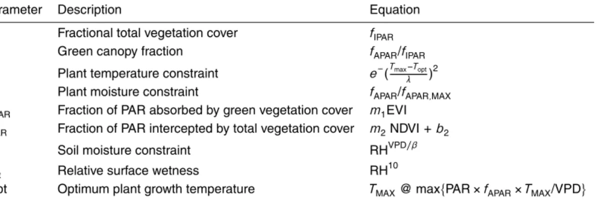
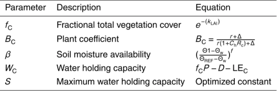
In this study, a remote sensing model of tran- spiration (the primary component of ET), driven by a time series of vegetation indices, was used to substitute transpi- ration from

and Wood, E.: The assimilation of remotely sensed soil brightness temperature im- agery into a land surface model using ensemble Kalman filtering: a case study based on

The objectives of this study are to assessment soil loss by using Geographic Information System and Remote Sensing technology and to determine the effect of land

Spatial distributions of remote sensing based GVF, ISA, albedo, and LAI (a, e, i and m) compared with those based on Noah/UCM lookup tables (b, f, j and n) and simulated maps
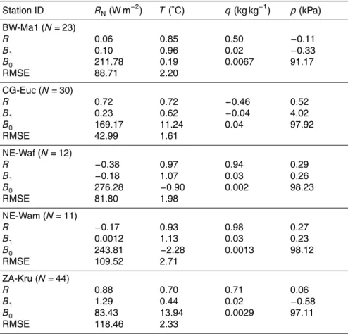
Land data assimilation systems (LDAS) are needed to integrate satellite data providing information about land state variables such as the surface soil moisture (SSM) and leaf area

Three different data products from the SMOS mission are assimilated separately into the GEOS-5 land surface model to improve estimates of surface and root-zone soil moisture and

In this study, the dynamic vegetation model Inland (Integrated Model of Land Surface Processes) driven by two representative concentration pathways (RCPs) scenarios was applied