of the optimal treatment neighborhood depend on the epidemiological factors. The required extent of prevention is proportional to the size of the infection neighborhood, but depends on time till detection and time till treatment in a non-nonlinear (power) law. The optimal size of control neighborhood is also highly sensitive to the relative cost, particularly for inefficient detection and control application. These results have important consequences for design of prevention strategies aiming at emerging diseases for which parameters are not nessecerly known in advance.
Citation:Oles´ K, Gudowska-Nowak E, Kleczkowski A (2012) Understanding Disease Control: Influence of Epidemiological and Economic Factors. PLoS ONE 7(5): e36026. doi:10.1371/journal.pone.0036026
Editor:Yamir Moreno, University of Zaragoza, Spain
ReceivedOctober 3, 2011;AcceptedMarch 26, 2012;PublishedMay 9, 2012
Copyright:ß2012 Oles´ et al. This is an open-access article distributed under the terms of the Creative Commons Attribution License, which permits unrestricted use, distribution, and reproduction in any medium, provided the original author and source are credited.
Funding:Project operated within the Foundation for Polish Science International Ph.D. Projects Programme co-financed by the European Regional Development Fund covering, under the agreement no. MPD/2009/6, the Jagiellonian University International Ph.D. Studies in Physics of Complex Systems. The project was carried out within the MPD programme "Physics of Complex Systems" of the Foundation for Polish Science and cofinanced by the European Development Fund in the framework of the "Innovative Economy Programme" and within the framework of "Exploring the Physics of Small Devices (EPSD)" of European Science Foundation (ESF). The funders had no role in study design, data collection and analysis, decision to publish, or preparation of the manuscript.
Competing Interests:The authors have declared that no competing interests exist.
* E-mail: [email protected]
Introduction
The network-based approaches are a common tool in epidemi-ological studies [1]. These individual-based methodologies allow incorporating the diverse patterns of interaction that underlie disease transmission and have been proved to capture topology of populations [2,3]. An interesting aspect of such studies, with an obvious goal to target spread of the disease, is identification of optimal strategies for the control of a disease under additional constraints [4–6]. Network modelling has been successfully used for many systems in order to design such control strategies [7]. However, there are only very few attempts to incorporate economic factors in such realistic models. Conversely, bioeco-nomic models usually ignore the spatial components of the disease spread [8–10].
In this paper we present a combined epidemiological and economic model to address the problem of optimization of disease control on networks with incomplete knowledge. Two main sources of costs can be associated with a disease outbreak and its control: the palliative cost associated with disease case and costs of measures aimed at preventing further cases [11,12]. The objective of preventive actions is to lower the total cost by investing e.g. in vaccination at the initial stages of the epidemic or culling of infected/susceptible individuals.
In our approach, we define a measure of the total cost of the epidemic (the severity index,X) and analyze the influence of the
parameters on its minimum. Work so far has shown that it is possible in such models to find an optimal control strategy [12]. Three optimal control scenarios (Global Strategy (GS), Local Strategy (LS), Null Strategy (NS)) emerge from the cost-effectiveness analysis. However, the relationship between the details of the Local Strategy and the model parameters is still elusive [7,12]. Establishing such a relationship is an essential step in designing control strategies for emerging diseases and hence we have concentrated on this task in the paper. We investigate propagation of the disease in a small-world network. The basic topology represents a regular lattice, with additional long-range bonds between randomly chosen pairs of sites. Inclusion of shortcuts into a regular lattice enhances communication of the disease and causes proliferation of epidemics at locations far apart from the original infected source.
We have found that the scale of control matches the scale of dispersal of a disease and so the larger the infection neighborhood, the further the control has to be extended. This relationship can be approximated by a linear function which coefficients depend algebraically on the detection and treatment rates following a power law. Small change in the relative cost of preventive to palliative treatment may result in big changes in this relationship. Addition of small world links narrows the range where the scaling (power) law is valid but the scaling persists for small values of detection and treatment times.
Methods
Model
We assume that individuals are located at nodes of a regular (square) lattice that represents geographical distribution of hosts. On this lattice, we define a local neighborhood of orderzas a von Neumann neighborhood in which we include z shells and w(z)~2z(zz1)individuals, excluding the central one. According-ly,z~0corresponds to a single individual, which means that this individual is not in contact with anyone,z~1corresponds to 4
nearest neighbors whilez~?corresponds to the whole popula-tion in the limit of infinite size of the system. For the small world model a fixed number of long range links has been added to the regular network described above. Those links span the whole population, but otherwise behave like local links.
The epidemiological model is a standard SIR (Susceptible-Infected-Removed) model [13], modified to include pre-symp-tomatic and symppre-symp-tomatic stages of the disease and to account for detection and treatment (cf. fig. 1). All individuals are initially susceptible (S) and the epidemic is initiated by introduction of several infected (I), pre-symptomatic individuals. Each of infected individuals (symptomatic and pre-symptomatic) stays in contact with a given (fixed) number of other individuals in its infection neighborhood of order zinf: After infection, the susceptible individual moves first to infected, pre-symptomatic class, (I) compartments. It can further infect its neighbors with probability
fper a contact but cannot be treated yet. As symptoms develop with probability q, individual moves to D class and can be detected. It is still infectious but can spontaneously recover with probabilityrand accordingly, move to a recovery class, (R) and cannot be further infected or treated.
Figure 1. Block diagram illustrating transitions in the model: transitions performed at each time step (blue solid lines) and transitions triggered by treatment (orange thin lines).
doi:10.1371/journal.pone.0036026.g001
Severity index, X/N
0 10
20 30
40 50 10-3
10-2 10-1
100
0 0.1 0.2 0.3 0.4 0.5 0.6 0.7 0.8 0.9 1
X/N
z
f
X/N
Figure 2. Severity index, X, as a function of the infection rate per contact fand the control neighborhood size z. Simulation
parameters:q~0:5,v,r~0:1with 40 initial foci and infected neighborhood size set tozinf~1,costc~1:
number of individuals in the population. In the above formulacrepresents a cost of treatment relative to the
cost of infection andzstands for the control neighborhood size.
0 10 20 30 40 50
Control size, zc
10-5 10-4
10-3 10-2
10-1 100
101 102
10310-4 10-3
10-2 10-1
100 0
10 20 30 40 50
zc
c f
zc
10-5 10-4
10-3 10-2
10-1 100
101
102 10310-4
10-3 10-2
10-1 100 0
10 20 30 40 50
zc
c f
zc
0 10 20 30 40 50
Control size, zc
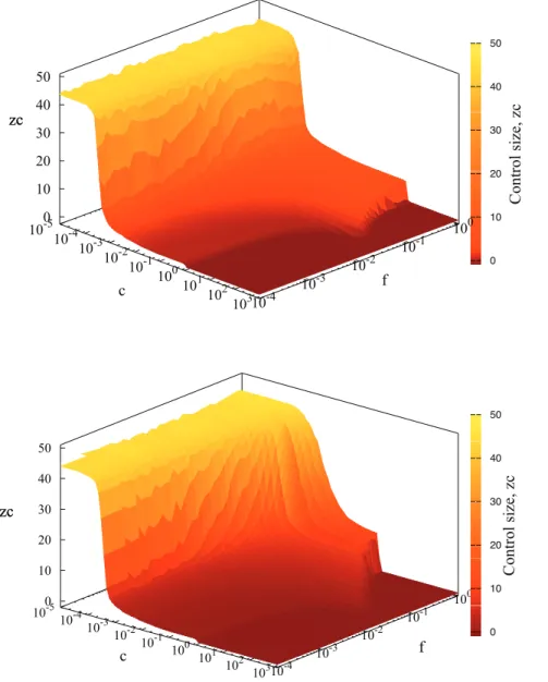
Figure 3. Control neighborhood size as a function of treatment costcand infectiousness of the diseaseffor regular network and
small world model.Simulation parameters:q~0:5,v,r~0:1,with 40 initial foci andzinf~1:Control sizezcw0represents local strategy (LS),zc~0
corresponds to the strategy when only the detected individual is treated andzc§30denotes GS (more than 99% of individuals are treated). Null
strategy corresponds tozc~{1:Top figure denotes results for disease spreading on regular networks, whereas bottom to small world model with
proved the consistency of results for different system sizes [12]. Epidemics have been initiated by addition of 40 infected individuals to an otherwise susceptible population. Each simula-tion run has been continued untilI(t)zD(t)~0 (i.e. up to the time when no further infection can occur). Subsequently the severity indexXhas been evaluated from the formula eq.(1). The optimal strategy is then determined by the minimal value of the severity indexXc:The corresponding value ofzgives the optimal size of the control neighborhood,zc(see fig. 2 for illustration). In the simulations, the minimization of the severity index is achieved by sweeping through different values of the control neighborhood sizez, while keeping other parameters fixed. For each value ofz
only a single simulation has been performed. Collections of this results yield a dependence ofXonz. A minimum value ofXin this collection gives an estimate ofXcand the correspondingzgives an estimate of zc:This procedure has been repeated 100 times to yield representative average values of zc and Xc and their corresponding standard deviations.
Results
The long time (t??) behavior of the model in the absence of control (Null Strategy, NS, i.e. z~{1) is determined by the probabilityfof passing the infection to a susceptible node from any of its neighbors within the neighborhood size ranging from 4 (z~1) to 144 (z~8). For small f, the infection quickly dies out. Disease spreads invasively over the population for largef, when no control is applied, X(z,?)!R(z,?)^N:Whenz§1, the ratio R=N declines with the order of the control neighborhood. However, at the same time the number of treated individuals V
increases, contributing to the total costX, cf. eq.(1). Forc=0,X(z)
is either a monotonic function ofzfor small values offor a non-monotonic function for highly contagious disease (largef), see fig. 2. Three regions can be identified in the dependence ofzconcand
f, see fig. 3. For small values of c, Global Strategy (GS) is dominating, whereas for largec, it is best to refrain from treatment, Null Strategy (NS), fig. 3.
Although the location of the minimum of X(z) varies with increasingfandcvalues (see figs. 2, 3), a relatively wide plateau region with an almost constantzcdevelops for intermediate values of c and f and corresponds to the local strategy (LS), fig.3. The structure in fig. 3 is partially deformed by addition of long-range links, however, the plateaux persists for small values off.
We have therefore focused on the plateaux region (LS) ofzcand have explored its dependence on epidemiological parameters: zinf,q,v,with constantfandc. We have first explored dependence ofzcon the size of infection neighborhood forc~1,see fig. 4. The relationship can be accurately approximated by a linear function for a wide range of parameters, infectiousnessf(fig.4a), the rate at
detection of symptoms. Similarly,tv~1=vcan be interpreted as an average time till treatment.
Broadly speaking, zc increases with tq and tv, fig. 5. This is consistent with the following mechanism. Consider a single infected but pre-symptomatic individual. The disease focus centered on it will spread until appearance of symptoms after time tq: Thus, the longer it takes to discover symptoms of the disease, the farther the disease would spread from its original focus. As a consequence, the infected area becomes larger and so doeszc:Similarly, the longer time from detection until treatment, the further the disease moves away from original focus. As a result, the control size grows with increasing treatment time.
10
1
10
100
zc
1/q
a)
10
1
10
100
zc
1/v
b)
Figure 5. Relationship betweenzcandt
qin a) andt
vin b).Points
mark the simulation results and lines correspond to fitted functions: a): zc(tq)~aqtbq and b):zc(tv)~avtbv’ for red:zinf~1, navy blue: zinf~3,
blue:zinf~5,orange:zinf~8:
Intriguingly, it appears thatzcscales algebraically withtq(and withtv) following a power law:zc~aqtb
qandzc~avtb
’
v eq.(3) (see fig. 5) with exponents well below 1.
The exponentsb,b’are similar for a range of zinf within the plateaux regime of an optimal control radius of the epidemic, (see fig.3), i.e. forzint[½1,8,b[½0:14,0:25andb’[½0:10,0:27:.
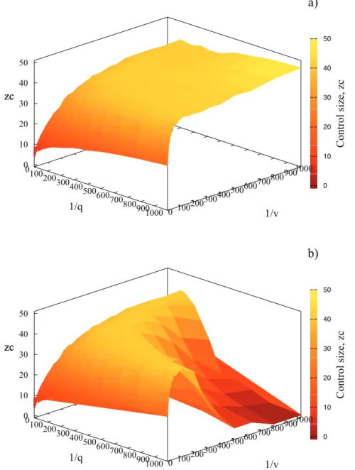
While fig. 5 is representative of results forcƒ1,moving cjust beyondc~1causes a dramatic change in thezc(tv)dependence for large values of tq and tv, corresponding to detection and vaccination time comparable with duration of epidemics (approx-imately 104time steps for large values oftv andtq). The control neighborhood zc decays abruptly for increasing timestq, tv,as illustrated in fig. 6. This change is associated with very inefficient control (long time till detection, tq&1 and long time from detection to treatment, tv&1). If the cost of control is lower or equal to the cost of palliative care, it is still better to treat, even
though we are not very efficient with treatment and most individuals are spontaneously removed. However, if the cost of vaccination is only marginally higher than the cost of untreated case, prevention is no longer cost-effective. We also note that it is only a combination of very long values oftqandtvthat leads to a limited range of application of the scaling formulas (zc~aqtb
qand zc~avtb’
v).
The scaling region ofzcas a function oftqandtcalso depends oncin a fashion reminiscent of fig. 3. For small values ofc, Global Strategy of treating everybody is optimal regardless of the parameters, cf. fig. 3 with fig. 7. In contrast, Null Strategy is optimal for largec(figs. 3 and 7). The region where Local Strategy is optimal occupies the region nearc~1,but it becomes narrower when the disease is more infectious (fig. 3) or when the control is less efficient (for increasing values oftq (fig. 7a) andtv (fig. 7b). Within this region,zcis given by scaling formulas. As seen before,
0 10 20 30 40 50
Control size, zc
0100 200300
400500 600700
800900
1000 0 100 200300 400500 600700 800900 1000 0 10 20 30 40 50
zc
a)
a)1/q
1/v
zc
0 10 20 30 40 50Control size, zc
0100 200300
400500 600700
800900
1000 0 100 200300 400500 600700 800900 1000 0 10 20 30 40 50
zc
b)
a)1/q
1/v
zc
Figure 6. Control neighborhood size as a function of both detection time,tq,and recovery time,tvforc~1in a) andc~1:001in b).
Simulation parameters:f~0:1,r~0:1,zinf~1,40 initial foci.
c~1is a special case asymptotically associated with a breakdown of LS for very large or very smallf(fig. 3) and very large values of tqandtv(fig. 7).
The addition of long range links shitfs the optimal radius of control towards larger values, figs. 3, 8. The scaling behaviour (cf. fig.5 ) is characteristic for a regular network and changes when long-range bonds is added (see fig.8). With 400 random long-range contacts (corresponding to 1% of all links) the scaling relation betweenzcandtq(tv) breaks down for detection (treatment) times exceeding 10. This is clearly indicated by deviation of the results from red bottom line (in fig.8) denoting simulation data for regular networks (the same as in fig. 5). Altogether, addition of small world links reduces the range of detectiontqand treatmenttvtimes for which the power law relationship is valid. This is caused by long range links allowing disease to escape from the local control. In contrast, if we are able to detect disease quicker, it has not much chance to escape and the disease spread is effectively short range. Consequently, the scaling can be observed for small values of detection and treatment times,tq,tv:In summary, with increasing degree of randomness of networks (larger number of links) not only the control radius rises but also the scaling disappears. Note that the dashed black line,zc~40in fig. 8, represents Global Strategy.
Discussion
In order to design a successful strategy for controlling a disease we need to take into account not only epidemiological and social factors (including the topology of the social network of contacts and in particularzinf), but also economic considerations. Some of these factors might be unknown or hard to estimate, particularly in real time as the epidemic unfolds. It is therefore crucial to understand the relationship between the optimal control strategy and parameters, for a wide range of possible values. It is even more important to establish those processes and parameters to which a selection of optimal strategy is not particularly sensitive, as this allows us to find strategies that can be designed in advance, even without knowing their actual values for a given emerging disease. Regular networks have been traditionally used for modelling epidemic outbreaks of human, animal and plant diseases [14,15] and many variants of such an approach (with e.g. constant or
10-4 10-3 10-2 10-1 100 101 102 103
0 10 20 30 40 50
b) zc
a)
10-4 10-3 10-2 10-1 100 101 102 103
Treatment cost, c
100
101
102
103
Treatment time, 1/v
Figure 7. Control neighborhood size as a function of treatment
cost c and detection time tq (a) and treatment time tv (b).
Simulation parameters:f~1,q~0:5,v,r~0:1, with 40 initial foci and zinf~1:Color borderlines between different regions indicate transition
regions among various optimal strategies. doi:10.1371/journal.pone.0036026.g007
1 10 100 1000
Detection time, 1/q
10
1 10 100 1000
O
p
ti
ma
l
co
n
tro
l
si
ze
,
zc
Treatment time, 1/v
Figure 8. Relationship between zc and tq on top and tv on
bottom for regular and small world network with varying
number of long-range links. Lines and simulation points from
bottom: red: regular network, navy blue: small world with additional 1% of links, green: small world with additional 5% of links, grey: small world with additional 10% of links, dashed black:zc~40which corresponds to
treating the whole population. Simulation parameters:f~1,v,r~0:1,
zinf~1,40 initial foci,1%,5%,10%of long-range links.
randomized probabilities of infection passed to neighbouring nodes on a grid) have been studied. However, an accumulated experimental evidence demonstrates that real systems rarely follow this kind of idealization being neither completely random nor located on regular lattices. Among other types of networks that have been the object of intense studies are the small-world and scale-free networks. In particular, the small world network with randomly chosen shortcuts between the nodes, is considered a model well extrapolating between extremes like regular and random network. It has been also preferentially used by modellers discribing outbreaks of disease starting simultaneously in different regions of the world (propagation of the SARS virus, [16]. Accordingly, in order to assess the occasional long distance dispersal of the disease, we have also considered small world links, representing e.g. random transport by wind or by plane.
In our previous paper we have shown that for a given set ofzinf, q and v, the broad choice of the strategy is determined by the relative cost of the treatment, c. For small values of c, GS is optimal, for large values ofc, NS. Close toc~1,a LS dominates and the detailed value of the control neighborhoodzcdepends on the epidemiological parameters, although not onfin a wide range. In this paper we extend this analysis to include other epidemio-logical parameters. In particular we show that the broad division between GS (forc%1), NS (forc&1) and LS (forc^1) holds for a
wide range of parametersqandv(inverse of time to detection and inverse of time to treatment, respectively), fig. 7.
Three other key results emerge from our analysis. Firstly, it is very important to match scale of control to the scale of infection dispersal. This has already been seen in other papers [17], but this is the first time we show it for spatial control on networks in the presence of economic evaluation. However, we also show that the size of the control neighborhood is not just simply equal to the size of the infection neighborhood (see fig. 4 and compare the scale of horizontal and vertical axes). In the presence of pre-symptomatic individuals (tq&0) and in the face of delays associated with application of control (tv&0) we need to extendzc well beyond zinf: The relationship between zinf and zc is one of the key formulas for planning response to epidemics. It enables authorities to plan actions aiming at eradication of the disease by setting a sufficiently large – but not too large – zone of eradication around each detected case. Traditionally, such recommendations are based on the dispersal patterns of the disease, although increas-ingly simulation models are used. This procedure has led to establishment of the 1,900ft rule for citrus canker [18] whereby all citrus trees are cut down within this radius from every affected tree and the 3 km/10 km rule for foot-and-mouth disease [19].
However, our results show that the relationship betweenzcand zinf is non-trivial and in particular it involves non-linear functions oftqandtv:Although we are still far from being able to provide a formula relatingzc to all epidemiological parameters, our result stresses importance of using models to design control strategies [20].
We also show thatc~1is a special case. In particular, we show high sensitivity ofzc to changes incfor large values oftqandtv:
Thus, if the symptom detection time (tq) and reaction time (tv) are both long, small change incleads to very big changes inzc,see fig. 6 and 7. Without knowing the exact value ofcit is therefore very difficult to design the strategy in this case. Suppose we believe thatcw1and therefore we chose a small value ofzcbased upon fig. 6b. However, if in realitycƒ1(although very close to 1), zc should be close to 50 (fig. 6a). This shows the importance of knowing what the actual value of c is [12] estimated that for vaccinationc~0:01–0.85, but can be larger than 1 for culling.
In this paper we have used regular and small wold networks to describe the topology of interaction between individuals. Addition of small world links into population narrows the range where the scaling (power law) relationship ofzcontqandtvis valid but the scaling persists for small values of detection and treatment times. Our studies can also be extended in other ways. The current work assumes relatively short overall time length of each epidemic and so no discounting is applied when the costs and benefits are estimated. We also assumed that the strategy is unchanged throughout the epidemic and that the network structure is static and relatively simple. Each of these assumptions can be relaxed. Discounting is often used in economics, but we expect for it to have a small impact on our results. Adapting the strategy to the current status of the epidemic often leads to a bang-bang solution [21], similar to our distinction between NS and GS.
Finally, a lot of attention have been recently given to non-local and random networks (small-world or scale-free networks) [12,22], to dynamic networks [23], and networks with random parameters [24]. Further extension of this work to include static and dynamic disorder is in progress.
Acknowledgments
We are very grateful to Bartek Dybiec for useful discussions.
Author Contributions
Conceived and designed the experiments: AK KO. Performed the experiments: KO. Analyzed the data: KO EGN AK. Contributed reagents/materials/analysis tools: KO EGN AK. Wrote the paper: KO EGN AK.
References
1. Newman M (2010) Networks: an introduction. Oxford Univ Pr.
2. Keeling M (2005) Models of foot-and-mouth disease. Proceedings of the Royal Society B: Biological Sciences 272: 1195.
3. Gastner M, Newman M (2006) Optimal design of spatial distribution networks. Physical Review E 74: 016117.
4. Barrett S (2003) Global disease eradication. Journal of the European Economic Association 1: 591–600.
5. Rowthorn R, Laxminarayan R, Gilligan C (2009) Optimal control of epidemics in metapopulations. Journal of the Royal Society Interface 6: 1135. 6. Ndeffo Mbah M, Gilligan C (2010) Optimization of control strategies for
epidemics in heterogeneous populations with symmetric and asymmetric transmission. Journal of Theoretical Biology 262: 757–763.
7. Ferguson N, Donnelly C, Anderson R (2001) The foot-and-mouth epidemic in great britain: pattern of spread and impact of interventions. Science 292: 1155. 8. Klein E, Laxminarayan R, Smith D, Gilligan C (2007) Economic incentives and mathematical models of disease. Environment and Development Economics 12: 707–732.
9. Gersovitz M, Hammer J (2004) The Economical Control of Infectious Diseases*. The Economic Journal 114: 1–27.
10. Boccara N, Cheong K, Oram M (1994) A probabilistic automata network epidemic model with births and deaths exhibiting cyclic behaviour. Journal of Physics A: Mathematical and General 27: 1585.
11. Kleczkowski A, Dybiec B, Gilligan C (2006) Economic and social factors in designing disease control strategies for epidemics on networks. Arxiv preprint physics/ 0608141.
12. Kleczkowski A, Oles´ K, Gudowska-Nowak E, Gilligan C (2011) Searching for the most cost-effective strategy for controlling epidemics spreading on regular and small-world networks. Journal of The Royal Society Interface.
13. Anderson R, May R (1991) Infectious diseases of humans: dynamics and control. Wiley Online Library.
14. Jeger M, Pautasso M, Holdenrieder O, MW S (2007) Modelling disease spread and control in networks: implications for plant sciences. New Phytologist 174: 279–297.
15. Shirley M, Rushton S (2005) The impacts of network topology on disease spread. Ecological Complexity 2: 287–299.