EXTENSIONS OF CUTTING PROBLEMS: SETUPS*
Sebastian Henn and Gerhard W¨ascher**
Received May 3, 2013 / Accepted July 19, 2013
ABSTRACT.Even though the body of literature in the area of cutting and packing is growing rapidly, research seems to focus on standard problems in the first place, while practical aspects are less frequently dealt with. This is particularly true for setup processes which arise in industrial cutting processes whenever a new cutting pattern is started (i.e. a pattern is different from its predecessor) and the cutting equipment has to be prepared in order to meet the technological requirements of the new pattern. Setups involve the consumption of resources and the loss of production time capacity. Therefore, consequences of this kind must explicitly be taken into account for the planning and control of industrial cutting processes. This results in extensions to traditional models which will be reviewed here. We show how setups can be represented in such models, and we report on the algorithms which have been suggested for the determination of solutions of the respective models. We discuss the value of these approaches and finally point out potential directions of future research.
Keywords: cutting, problem extensions, setups, exact algorithms, heuristic algorithms, multi-objective optimization.
1 INTRODUCTION
The body of literature on cutting and packing (C&P) problems is still rapidly growing. In order to provide an instrument for the systematic organisation and categorisation of existing and new literature in the field, W¨ascheret al. (2007) introduced a typology of C&P problems in which the criteria for the definition of homogeneous problem categories are related to “pure” problem types,i.e.problem types of which a solution comprises information on the set of cutting/packing patterns, the number of times they have to be applied, and the corresponding objective function value, only.
Cutting and packing problems from practice, on the other hand, are often tied to other problems and cannot be separated from them without ignoring important mutual interdependencies. Re-alistic solution approaches to such integrated problems, therefore, do not only have to provide
*Invited paper **Corresponding author
cutting patterns, but also have to deal with additional problem-relevant aspects such as process-ing sequences (as in the pattern sequencprocess-ing problem; cf. Foerster & W¨ascher, 1998; Yanasse, 1997; Yuen, 1995; Yuen & Richardson, 1995), due dates (cf. Helmberg, 1995; Li, 1996; Rein-ertsen & Vossen, 2010; Rodriguez & Vecchietti, 2013), or lot-sizes (cf. Non˚as & Thorstenson, 2000). In this paper, we address the issue of setups which arise in industrial cutting processes whenever a new cutting pattern is started (i.e.a pattern is different from its predecessor) and the cutting equipment has to be prepared in order to meet the technological requirements of the new pattern. Setups of this kind involve the loss of production time capacity and the consumption of resources which can be avoided or, at least, reduced by taking into account theses consequences when decisions are made on the set of cutting patterns to be applied.
Setups represent an important issue of real-world (extended) cutting problems but have only been considered occasionally in the literature related to C&P problems. We, therefore, would like to give an overview of the state-of-the-art in the field, but also to emphasize theoretical deficiencies and future research opportunities. We restrain our analysis to papers which are publicly available and have been published in English in international journals, edited volumes, and conference proceedings between by the end of 2012.
2 FUNDAMENTALS
2.1 Cutting and Packing Problems – Definition and Typology
The general structure of cutting and packing problems can be summarised as follows (in the following, in particularcf.W¨ascheret al., 2007):
Given are two sets of elements, namely
• a set of large objects (supply) and
• a set of small items (demand),
which are defined exhaustively in one, two, or three (or an even larger number) of geometric dimensions. Select some or all small items, group them into one or more subsets and assign each of the resulting subsets to one of the large objects such that thegeometric conditionholds,i.e.
the small items of each subset have to be laid out on the corresponding large object such that
• all small items of the subset lie entirely within the large object and
• the small items do not overlap,
and a given objective function is optimised.
With respect to standard problems, basically two types of assignment can be distinguished. In the case of input (value) minimization, the set of large objects is sufficient to accommodate all small items. All small items are to be assigned to a selection (a subset) of the large object(s) of minimal value. There is no selection problem regarding the small items.
In the case of output (value) maximisation, the set of large objects is not sufficient to accommo-date all the small items. All large objects are to be used, to which a selection (a subset) of the small items of maximal value has to be assigned. There is no selection problem regarding the large objects.
Depending on the specific problem environment, the “value” of objects/items has to be defined more precisely and may be represented by costs, revenues, or material quantities. Often, the value of the objects/items can be assumed to be directly proportional to their size such that the objec-tive function considers length (one-dimensional problems), area (two-dimensional problems), or volume (three-dimensional problems) maximization (output) or minimization (input). In such cases, both “output (value) maximization” and “input (value) minimization” may be replaced by “waste minimization”, i.e. the minimization of the total size of unused parts of the (selected) large objects. In the environment of cutting problems often the term “trim-loss minimization” is used.
The determination of cutting patterns and the corresponding application frequencies represent the core elements in solving cutting problems. Despite of having the above-described problem structure in common, actual cutting problems may be quite different in detail and do not allow for being treated by the same or even similar solution approaches. In order to define more homoge-neous problem types, W¨ascheret al.(2007) – apart from “kind of assignment” use two additional criteria, namely”, “assortment of large objects” and “assortment of small items”, in order to iden-tify 14 (intermediate) problem types. By means of two additional criteria, “dimensionality” and “shape of small items” further refined problem types can be obtained.
2.2 Setups
Realistic solution approaches to cutting problems in practice do not only have to provide cutting plans, but also have to deal with additional aspects and have to answer additional questions. One such aspect concerns the setups which may arise in industrial cutting processes whenever a new cutting pattern different from its predecessor is started and the cutting equipment has to be prepared in order to meet the technological requirements of the new pattern. Setups of this kind involve the loss of production time capacity and the consumption of resources.
• In the paper industry, reels in sizes demanded by customers are to be cut from large pa-per rolls (jumbos). This is carried out on a so-called winder which unwinds a jumbo and rewinds it on cores while the paper is being slit. The slitting itself is done by means of rotating knifes or laser beams which have to be repositioned whenever a new cutting pat-tern is started. In order to do so, the winder has to be stopped and the paper has to be fed in again. After the winder has been restarted the paper may take some time to settle in, during which defects can occur (cf.Diegelet al., 2006, p. 708f.).
• Kolen & Spieksma (2000) describe a similar setting related to the production of abrasives. Abrasives are also manufactured in rolls (raws) which have to be cut down into rolls of smaller widths ordered by external customers. Apart from minimizing the trim loss, the company also seeks to minimize the number of different cutting patterns since the cutting machine undergoes a setup every time two consecutive raws have to be cut according to different patterns. Setting up the machine is a manual, time-consuming operation. The authors mention that a setup might require up to three quarters of an hour.
• In the corrugated cardboard industry, a similar technology (rotating knifes) is used for slit-ting the final product into smaller widths (demanded by external customers or required by subsequent internal production stages). The slitting of the cardboard follows immediately after the actual production process. The production process itself is a continuous one and cannot be interrupted,i.e.while the knifes are being repositioned for a new cutting pattern, cardboard keeps shooting out of the production facility without being cut. It can only be treated as waste and has to be disposed at additional costs (cf. Pegels, 1967; Haessler & Talbot, 1983).
Hajizadeh & Lee, 2007). The machine operates a number of knives in parallel or succes-sively after one another. Typically, the entire cutting process needs to be stopped in order to change the complete set or a subset of the used knives, or some knife positions.
Aiming entirely at a minimization of input, it cannot be expected that traditional approaches to cutting processes will always give satisfactory results under these conditions since input min-imization on one hand and setup minmin-imization on the other are conflicting goals (cf., among others, Farley & Richardson, 1984, p. 246; Vanderbeck, 2000, p. 916; Umetaniet al., 2003a, p. 1094; Umetaniet al., 2006, p. 45; Cuiet al., 2008, p. 677; Moretti & de Salles Neto, 2008, p. 63). Instead, it would be useful to reduce the number of cutting patterns (and, by doing so, the number of setups) in a solution at the expense of additional input or trim loss if that would result in a reduction of the respective total costs. Consequently, the inclusion of setups represents a straightforward extension to the traditional input minimization models.
3 THE SINGLE STOCK SIZE CUTTING STOCK PROBLEM (SSSCSP)
Of all 14 intermediate problem types identified by W¨ascheret al. (2007), theSingle Stock Size Cutting Stock Problem(SSSCSP) is of particular interest, because the literature to be reviewed here is related to problems of this kind in the first place. In this section, the SSSCSP will be defined and it will be shown how it can be modeled. The models which will be presented are general in the sense that they represent one-dimensional, two-dimensional and three-dimensional cutting problems with small items of any shape.
3.1 Problem Formulation
The SSSCSP can be stated as follows: A weakly heterogeneous assortment of small items has to be cut from a stock of large objects, which are available in a sufficiently large number of identical pieces of a single given (standard) size. The number of the large objects needed to provide all small items has to be minimized.
3.2 Two Models for the SSSCSP
In the following, we introduce the notation for a formal representation (model) of the SSSCSP.
I: set of all small item types which have to be cut,I = {1,2, . . . ,m};
J: set of all (relevant) cutting patterns which can be applied to the large object type in order to cut it down into small items;
ai j: number of times small item type i(i ∈ I) appears in cutting pattern j (j ∈ J);
di: demand for small item type i(i ∈ I); number of times small item type i(i ∈ I)has to be provided;
tj: trim loss per large object involved with cutting pattern j(j∈ J);
By means of these symbols, the SSSCSP can then be represented by model M 1.1 of Table 1, which we call theInputMinimizationModel of the SSSCSP(IMM) here. The objective function (3.1) postulates a minimization of the total number of large (stock) objects (input minimization) which is necessary to satisfy all demands. Demand constraints (3.2) guarantee that (at least) the demanded number of items of each small item type is provided. Integer constraints (3.3) make sure that large objects are always cut down completely.
Waste may occur as trim loss contained in the selected cutting patterns (i.e.parts of a large object which are not covered by small items), but also as excess production (surplus) which is provided beyond the actual demand of the small item types. Since all demands are fixed and have to be satisfied exactly, input minimization and waste minimization are equivalent goals.
All large objects are identical, not only with respect to their size but also with respect to their material cost. Therefore, minimization of the material (input) quantity (i.e. minimization of the number of large objects) will also result in a minimization of the total material (input) cost. Alternatively, instead of input minimization, one may also chose trim loss minimization as a goal. The corresponding model is given by M 1.2 (TMM:Trim Loss MinimizationModel of
the SSSCSP) of Table 1. The objective function (3.4) calls for a minimization of the total trim loss. Since, according to constraints (3.5), the small item types have to be provided exactly in the demanded quantities, no excess production can occur. In other words, a trim loss minimal solution of (3.5) and (3.6) is also a waste minimal solution. Consequently, M 1.1 and M 1.2 are equivalent models. Optimal solutions of M 1.1 on one hand and of M 1.2 on the other will possess the same amount of input and the same amount of waste, even though not necessarily the same amount of trim loss.
Table 1– Basic Optimization Models for the SSSCSP.
Basic Optimization Models Input Minimization (M 1.1) IMM
X
j∈J
xj →Min! (3.1)
X
j∈J
ai j∙xj ≥di, i∈I; (3.2)
xj ≥0, integer, j∈ J. (3.3)
Trim Loss Minimization (M 1.2) TMM
X
j∈J
tj∙xj →Min! (3.4)
X
j∈J
ai j∙xj =di, i∈I; (3.5)
We note that, due to the fact that excess production is permitted, with respect to model M 1.1, it is sufficient to consider complete patterns (i.e. patterns to which no further small item can be added) only in the set J of cutting patterns, while in M 1.2 – due to the equations in (3.5) – J must also include all incomplete patterns. The same applies to model M 1.1 if the demand constraints (3.2) are formulated as equations (as,e.g.in Vanderbeck, 2000, p. 915).
Goulimis (1990, p. 203) argues that equality-constrained optimization models are more difficult to solve and tend to give patterns with trim loss unacceptable in practice. Therefore, he and sev-eral other authors (e.g.Haessler, 1975, 1988; Vaskoet al., 2000) allow for demand tolerances,i.e.
demands which only have to be satisfied within certain pre-specified limits, instead of demands which have to be satisfied exactly. Constraints (3.5) are replaced by constraints of the type
min(di)≤ X
j∈J
ai j ∙xj ≤max(di), j ∈ J. (3.7)
From an economist’s point of view, this is not totally convincing. Since both input and output of the cutting process are now variable, it would formally be necessary to introduce profit maxi-mization as a goal in the corresponding objective function. Such modifications are not common in the literature, though. Among the few exceptions is a paper of Schilling & Georgiadis (2002), who develop an even more general model which does not only comprise the revenues from the provided small items (final products), the cost of the large objects (material cost) and the cost of setups, but also explicitly considers the cost of disposing the trim loss.
We would also like to point out that further modeling approaches to the SSSCSP exist, namely the one-cut model of Rao (1976) and Dyckhoff (1981) and the network flow model of Val´erio de Carvalho (1998). We do not present any further details of these models here, since they are less suitable for being extended for the inclusion of setup aspects.
3.3 Solution Approaches
When given a particular problem instance of the SSSCSP, one may immediately think of generat-ing the respective model M 1.1 or M 1.2 and have it solved by a commercial LP solver. This is, in fact, a solution approach which is occasionally taken in practice when the number of item types is small and/or when special constraints of the cutting technology limit the number of feasible cutting patterns to a small number (cf. Kochet al., 2009). In general, this approach will not be feasible, though, since the number of cutting patterns and, likewise, the number of variables in the corresponding model, grows exponentially with the number of different item types and very easily reaches prohibitive dimensions.
straightforward approach for the generation of an integer solution consists of rounding up the non-integer application frequencies of the cutting patterns to the next integer. This immediately gives a feasible solution to the original problem (as stated in Section 3.1) while rounding down does not, since demand constraints will be violated. The drawback of this simple procedure lies in the fact that the true input-minimal or trim loss-minimal solution will usually be missed, probably by far. On the other hand, by means of Branch-and-Bound or sophisticated rounding techniques (W¨ascher & Gau, 1996) applied to the non-integer solution, an input-minimal or trim loss-minimal solution can be identified, but usually at the expense of additional cutting patterns/setups in the solution.
Thus it is not surprising that when one has to deal with setups, certain heuristic approaches are often used which have been popular in the early days of applying operations research methods to cutting problems and which have been proven flexible enough to incorporate additional practical requirements. Methods of this type are usually based on theRepeated Pattern Exhaustion Tech-nique(RPE Technique; Dyckhoff, 1988) for the (heuristic) solution of cutting problems. This is a sequential solution approach (usually described for the one-dimensional SSSCSP) in which cutting patterns and the frequencies according to which they are admitted into the cutting plan are determined successively. It consists of three phases: (1) generation of an “acceptable” cutting pattern j, (2) determination of the maximal frequencyxj according to which the pattern can be applied (limited by the remaining demands), and (3) update of the demands. These phases are repeated until all demands are satisfied (cf. Pierce, 1964, p. 28ff.). Integrality of the generated solution can be guaranteed easily in step 3.
4 TOTAL COST MINIMIZATION FOR THE SSSCSP WITH SETUPS
4.1 Total Cost Models
The IMM can be extended in a straightforward way in order to take into account for setups by switching to an objective function which aims at minimizing the total decision-relevant cost. We introduce the following additional symbols:
cINPUT: cost per large object; cSETUP: cost per setup;
cTRIM: cost per unit of trim loss;
M: sufficiently large number (“Big M”); δj: binary variable with
δj = (
1, if cutting pattern j(j ∈ J)is used, 0, else.
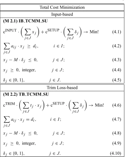
Model M 2.1 of Table 2 represents theInput-BasedTotalCostMinimizationModel of the
Table 2– Total Cost Minimization Models of the SSSCSP with Setups.
Total Cost Minimization
Input-based (M 2.1) IB TCMM SU
cINPUT∙
X
j∈J
xj
+cSETUP∙
X
j∈J δj
→Min! (4.1)
X
j∈J
ai j∙xj ≥ di, i∈ I; (4.2)
xj−M∙δj ≤ 0, j∈ J; (4.3)
xj ≥ 0, integer, j∈J; (4.4)
δj ∈ {0,1}, j∈J. (4.5)
Trim Loss-based (M 2.2) TB TCMM SU
cTRIM∙
X
j∈J
tj∙xj
+cSETUP∙
X
j∈J δj
→Min! (4.6)
X
j∈J
ai j∙xj =di, i∈I; (4.7)
xj−M∙δj ≤ 0, j∈ J; (4.8)
xj ≥ 0, integer, j∈J; (4.9)
δj ∈ {0,1}, j∈J. (4.10)
For any solution of the optimization model M 2.1, P
j∈Jδj will give the number of cutting patterns and, equivalently, the number of setups. Consequently, the objective function (4.1) now includes the total cost of the utilized large objects (input cost; basically consisting of material cost) and the total cost of setups. Obviously, an implicit assumption of this model is that the cost for setting up the cutting equipment is proportional to the number of setups, but independent from the respective pattern and also from the preceding and the succeeding pattern. (4.8) are auxiliary constraints in which M is a sufficiently large number. Each of these constraints – in combination with the minimization instruction for the objective function value – guarantees that the binary variable δj corresponding to cutting pattern j(j ∈ J)is set to one and the setup costs are included in the calculation of the objective function value whenever cutting pattern jis actually used.
Likewise, one may also take the TMM as the basic model and extend it with respect to the number of cutting patterns. This gives rise to theTrim Loss-BasedTotalCostMinimizationModel of
the cutting pattern applied to a large object. In that case, in the objective function the constant cINPUThas to be omitted and thetj-coefficients have to be replaced by the corresponding costs cjrelated to cutting one large object according to pattern j.
4.2 Solution Approaches
The solution approaches to be presented here are all of the heuristic type. Unlike the methods to be discussed in the subsequent sections, they all assume that the relevant cost information is available and make explicitly use of this information for the generation of solutions.
Farley & Richardson (1984) present a heuristic for the two-dimensional TB TCMM SU which is based on the column-generation approach by Gilmore & Gomory (1965). It starts from an optimal solution of the continuous relaxation of the SSSCSP and, in a series of iterations, tries to reduce the number of structural variables (i.e. the number of different patterns) in the solution. Unlike in the Gilmore-Gomory approach, variables corresponding to cutting patterns are not discarded as they are leaving the basis. The authors give (heuristic) rules according to which basic structural variables and non-basic slack variables should be swapped. The method generates a sequence of feasible, not necessarily integer basic solutions and terminates when no improved or feasible solution can be found.
The authors have evaluated the proposed method on fifty two-dimensional problem instances with twenty small item types each. For (relative) values of the pattern cost (cost of trim loss per pattern) over the setup cost ranging from 1:0 up to 1:20 they demonstrated how the proportion between waste and number of patterns changed in the respective best solution. The question of generating integer solutions was not specifically addressed. In principle, the proposed method can also be applied to the one- and three-dimensional SSSCSP with identical setups.
Jardim Campos & Maculan (1995) consider the one-dimensional IB TCMM SU. They drop the integer constraints (4.4) for the xj variables and derive the Langrangian dual of the remain-ing optimization problem. This problem may be solved by subgradient methods into which the column-generation technique of Gilmore & Gomory (1961, 1963) has been integrated. No nu-meric example is given and no computational experience is reported. The question of how integer solutions can be generated is not addressed.
Diegel et al. (1996b) discuss an extensive numerical example for the one-dimensional IB TCMM SU. On the basis of an explicit model formulation they exemplify the necessity to consider setups in the planning process and discuss how appropriate (relative) cost factors (pat-tern costs, setup costs) can be chosen when the exact ones are not known. They do not address any computational aspects related to problem instances which result in models too large for be-ing solved by commercial optimizers, or for which the explicit models cannot even be generated (because they contain too many columns).
which establishes a (column) basis of the coefficient matrix of the constraint system (3.2). It is solved by means of an augmented Lagrangian method. The pricing problem consists of a bounded knapsack problem; the respective simplex multipliers are determined by solving another linear optimization problem of the type (3.4)-(3.6), where the coefficients tj are computed from the values of cINPUT and cSETUP, and the application frequenciesxj of the current solution of the master problem. It is solved in order to determine a new column (cutting pattern) which would improve the current objective function value of the master problem. If such a column is identified, it enters the basis and the master problem is solved again. The solution of the master problem is recorded if it is better – with respect to (4.1) – than the solutions generated from the master problem in previous iterations. These steps are repeated until the pricing problem provides no further column that would improve the current solution of the master problem. The initial set of cutting patterns is determined by theSequential Heuristic Procedureof Haessler (1975). Integer solutions are obtained from the best recorded solution by application of the BRURED rounding procedure (Neumann & Morlock, 1993, p. 431f.; W¨ascher & Gau, 1996, p. 134), which may result in excess production but does not increase the number of cutting patterns in the solution. The authors have tested their approach (NANLCP) on a set of randomly generated problem instances from Foerster & W¨ascher (2000), which includes 18 problem classes with 100 instances each. For cINPUT =1 and cSETUP=5 they found that NANLCP obtained solutions with lower average total cost than KOMBI234 (i.e.the method proposed by Foerster & W¨ascher, 2000) does for 15 problem classes. For cINPUT =1 and cSETUP=10 NANLCP outperformed KOMBI234 for all 18 problem classes. On the other hand, computing times for NANLCP were significantly larger than for KOMBI234 and seem to represent a major drawback of the proposed method (cf. Moretti & Salles Neto, 2008, p. 76f.) We further note, that KOMBI234 is a method based on the (implicit) assumption that cINPUT≫cSETUP(see below). Therefore, we conclude that the results from the numerical experiments with NANLCP on one hand, and with KOMBI234 on the other cannot really be compared to each other.
the best solutions. In the evolutionary process these patterns are meant to generate other patterns which will provide even better solutions.
The authors have run numerical experiments similar to the ones of Moretti and Salles Neto (2008). In particular, the 18 classes of randomly generated problem instances from Foerster & W¨ascher (2000) were considered again. For cINPUT = 1 and cSETUP = 1 they found that the SGA outperformed KOMBI234 on one and NANLCP on seven problem classes. For cINPUT=1 and cSETUP = 5, in comparison to KOMBI234, the SGA provided smaller average costs per problem instance for ten problem classes, and in comparison to NANLCP for four classes. For cINPUT =1 and cSETUP =10 better solutions (on average) were found for 14 problem classes (KOMBI234) and six classes (NANLCP), respectively. The computing times were significantly larger than those for KOMBI234 (with the exception of one problem class) and NANLCP, and ranged from 17.66 to 426.08 seconds per instance (for cINPUT = 1, cSETUP = 5) on a AMD SEMPRON 2300+ PC (1.5 MHz, 640 MB RAM). We remark that the numerical experiments also included a comparison of the SGA to the ILS approach of Umetaniet al.(2006) and to the heuristic of Yanasse & Limeira (2006). We do not report the results here since we believe that, again, these methods belong to different classes of methods (see below) and, thus, the results are not really comparable.
Atkin & ¨Ozdemir (2009) refer to a one-dimensional cutting problem in coronary stent manufac-turing. The proposed solution approach consists of two phases. In the first phase, a heuristic is applied in order to generate a set of trim-loss minimal cutting patterns. In the second phase, these patterns are used for setting up a model of the IB TCMM SU type from which the respective frequencies of application are determined. The model is more complex than the above-presented one. Apart from input (material) and setup costs, it also incorporates labor cost for regular work-ing hours and overtime, and costs of tardiness. By means of numerical experiments the authors demonstrated that – under conditions encountered in practice – the heuristic from the first phase already gives satisfactory results when used as a stand-alone procedure and, thus, may not neces-sarily be accompanied by the succeeding linear programming approach form the second phase.
5 INPUT OR TRIM LOSS MINIMIZATION SUBJECT TO SETUP LIMITATIONS
Given that the cost coefficients of the total cost models M 2.1 and M 2.2, namely the cost per large object cINPUT, the cost per unit of trim-loss cTRIM and the cost per setup cSETUP, are not always known in practice, instead of minimizing the total cost as defined in (4.1) and (4.6) one may turn to limiting one of the underlying cost drivers to a specific maximal amount while the amount of other one is tried to be kept as small as possible. In the following, we will first deal with minimizing the input or the trim loss subject to a given number of setups.
5.1 Setup-Constrained Input or Trim Loss Minimization Models Let the following additional notation be introduced:
Then, on the basis of the IB TCMM SU, aSetup-ConstrainedInputMinimizationModel of the
SSSCSP withSetups (SC IMM SU) can be obtained if we replace objective function (4.1) in Model M 2.1 by
X
j∈J
xj →Min! (5.1)
and add the following constraint
X
j∈J
δj ≤max(s) (5.2)
which limits the number of cutting patterns in the solution to an acceptable number max(s). Umetaniet al.(2003a, p. 1094) also call this problem thePattern-Restricted Version of the Cut-ting Stock Problem.
Likewise, a Setup-Constrained Trim Loss Minimization Model of the SSSCSP with Setups (SC TMM SU) can be formulated if – in Model M 2.2 – the objective function (4.6) is replaced by
X
j∈J
tj∙xj →Min! (5.3)
and constraint (5.2) is added.
5.2 Solution Approaches
another pattern. The ILSA terminates if no improvement has been obtained for a pre-specified number of iterations.
The authors have performed numerical experiments in which the ILSA was evaluated in com-parison to Haessler’s RPE Technique (SHP) and KOMBI234 on the 18 classes of randomly generated problem instances of Foerster & W¨ascher (2000). For all problem classes they found that the (average) minimum number of setups generated by the ILSA was significantly smaller than the number of setups provided by KOMBI234, while the (average) amount of input was significantly larger. The same was true in comparison to SHP, which turned out to be dominated by KOMBI234, the latter providing solutions with fewer setups and smaller amounts of input (averages per problem class) than SHP. The average computing time per problem instance ranged between 0.05 and 70.25 seconds on a Pentium III/1GHz PC with 1GB core memory.
In a subsequent paper (Umetani et al., 2006), the authors present an improved ILSA. As an additional feature, they introduce a second neighborhood structure (called shift neighborhood) which is applied alternately in the local search phase. It is defined by exchanging one small item in a cutting pattern with one or several other items from another pattern. After a local optimum has been found, the local search phase is started again from a randomly selected solution of the shift neighborhood. Results from numerical experiments demonstrate that this improved ILSA generates solutions with smaller amounts of trim loss for the same number of patterns.
Different to the model presented above, Umetani et al. (2003b) consider a variant of the SC TMM SU, in which they allow both surplus and shortage with respect to the demands, and they search to minimize the quadratic deviation of the provided small items from their respective demands for a given number max(s)of cutting patterns. It is interesting to note that their problem formulation does not explicitly consider the trim loss. For the stated problem, they present an algorithm (ILS-APG) which is based on Iterated Local Search. A neighborhood solution is ob-tained by replacing one cutting pattern in the current solution by another one, which is generated by an adaptive pattern generation technique. In order to evaluate the new solution, the appli-cation frequencies of the cutting patterns are determined by a heuristic based on the nonlinear Gauss-Seidel method.
The proposed method has been tested on the randomly generated instances of Foerster & W¨ascher (2000) and a set of instances taken from a practical application at a chemical fiber company in Japan and run against SHP and KOMBI234. The authors claim that their method provides comparable solutions, even though it must be remarked that the results are not com-pletely comparable due to the fact that ILS-APG – unlike SHP and KOMBI234 – permits surplus and shortages.
6 SETUP MINIMIZATION SUBJECT TO INPUT OR TRIM LOSS LIMITATIONS
In contrast to the models and solution approaches presented in the previous section, one may minimize the number of setups subject to an acceptable level of input or trim loss.
max(o): maximal number of large objects permitted in a solution; max(t): maximal (total) amount of trim loss permitted in a solution.
Then, on the basis of the IB TCMM SU, an Input-Constrained Setup Minimization Model
(IC SMM) can be obtained if we replace objective function (4.1) in model M 2.1 by X
j∈J
δj →Min! (6.1)
and add the following constraint:
X
j∈J
xj ≤max(o) . (6.2)
Likewise, on the basis of the TB TCMM SU we receive aTrim Loss-Constrained Setup Mini-mization Model(TC SMM) if we replace objective function (4.1) in model M 2.2 by (6.1) and add the constraint
X
j∈J
tj ∙xj ≤max(t) . (6.3)
The problem of minimizing the number of cutting patterns (setups) subject to a given number of large objects or a given amount of trim loss is also calledPattern Minimization Problem (Van-derbeck, 2000). We point out that some authors particularly assume that the respective number of large objects or the respective amount of trim loss is minimal (cf. McDiarmid, 1999, Alves & de Carvalho, 2008). This problem is strongly NP-hard, even for the special case that any two demanded items fit into the large object, but three do not (cf.McDiarmid, 1999).
6.2 Solution Approaches
Due to its NP-hardness, initially the Pattern Minimization Problem has usually been solved heuristically. We present these approaches first before we turn to more recent exact approaches.
6.2.1 Heuristic Approaches
be seen as a generalization of the method by Diegelet al.(1996a). It permits the combination ofp
patterns intoq(p>q;p,qinteger;q >2) and is based on the fact that the sum of the application frequencies of the resulting patterns has to be identical to the sum of the frequencies belonging to the original patterns in order to keep the input constant. In computational experiments, which included 18 problem classes with 100 instances each, Foerster & W¨ascher (2000) demonstrated that KOMBI is superior to the other methods of this approach. However, since only a limited number of all possibleptoq-combinations are checked, it cannot be expected that a solution with a minimum number of patterns is found in the end, i.e. the final solution does not necessarily represent an optimum in the lexicographic sense.
Burkard & Zelle (2003) consider a (one-dimensional) reel cutting problem in the paper indus-try which is characterized by several specific pattern constraints (maximum number of short items/reels in the pattern, maximum number of long items/reels in the pattern, minimum width of the pattern). They introduce a randomized local search (RLS) heuristic which is applied in two phases: In the first phase a near-optimal solution to the equality-constrained IMM is determined by means of move, swap (swap, swap2×1, swap2×2, swap2×1×1 exchanges) and normaliza-tion operanormaliza-tions and addinormaliza-tional “external” neighborhood moves. Since all feasible cutting patterns are considered, the solution is also near-optimal with respect to the trim loss. Then, in a second phase, the RLS heuristic – limited to a subset of the neighborhood moves – is applied in order to reduce the number of cutting patterns.
The authors have carried out numerical experiments with 6 problem instances from the paper industry. They have run their method against a software package which was used at the paper mill where the instances were obtained and achieved a significant reduction in the number of different patterns. (The authors also carried out additional experiments with the bin-packing instances from Falkenauer (1996) and from Schollet al.(1997). The results are not reported here because the authors do not give any information on the quality of the solutions with respect to the number of patterns.)
6.2.2 Exact Approaches
The first exact approach to the (one-dimensional) Pattern Minimization Problem (PMP), a branch-and-price-and-cut algorithm for the one-dimensional case, was proposed by Vanderbeck (2000). An initial, compact formulation of the PMP is reformulated by means of the Dantzig-Wolfe decomposition principle, resulting in an optimization problem where each column repre-sents a feasible cutting pattern associated with a possible application frequency. This problem is solved by a column-generation technique in which the pricing (sub-) problem is a non-linear pro-gram. The non-linearity is overcome by solving a series of bounded knapsack problems. Cutting planes based on applying a superadditive function to single rows of the restricted master problem are used to strengthen the problem formulation. A branch-and-bound scheme guides the search of the solution space.
the generation of the cutting planes is not maximal and, therefore, may be dominated by other superadditive functions.
Alves & de Carvalho (2008) present an exact branch-and-price-and-cut algorithm for the one-dimensional PMP, which is based on Vanderbeck’s model. The authors introduce a new bound on the waste, which strengthens the LP bound. It also reduces the number of columns to be generated and the corresponding number of knapsack problems to be solved in the column-generation process. Dual feasible functions described by Fekete & Schepers (2001) are used to derive valid inequalities superior to the cuts proposed by Vanderbeck. Furthermore, the authors formulate an arc-flow model of the problem which is used to develop a branching scheme for the branch-and-bound algorithm. Branching is performed on the variables of the model. The scheme avoids symmetry of the branch-and-bound tree.
Numerical experiments were run on a 3.0 Ghz Pentium IV computer, the time limit was set to two hours again. The proposed algorithm solved one additional instance of Vanderbeck’s set of test problem instances to an optimum. However, in comparison to Vanderbeck’s algorithm, the number of branching nodes needed for finding an optimal solution was reduced by 46 percent for these instances. The LP bound obtained by adding the new cuts was also improved significantly. At the root node, the improvement amounted to 21.5 percent on average. The algorithm was fur-ther evaluated on 3,600 randomly generated test problem instances, divided into 36 classes of 100 instances each. The experiments clearly demonstrated that the percentage of optimally solved in-stances drops sharply with an increase in the number of small item types. Form=40 only one third of the instances could be solved to an optimum within 10 minutes of CPU time. For the remaining instances, the average optimality gap was 12.1 percent. Also, an increase in the aver-age demandaver(d)= |1I|P
i∈Idi reduces the percentage of optimally solved instances. This can be explained by the fact that an increase inaver(d)will increase the application frequencies which, again, will increase the number of pricing problems to be solved.
Based on a different model, Alveset al. (2009) develop new lower bounds for the one-dimen-sional PMP. The model itself is an integer programming model and can be solved by column generation; constrained programming and a family of valid inequalities are used to strengthen it. In order to verify the quality of the new bounds, numerical experiments were conducted on the benchmark instances of Vanderbeck (2000) and a subset of the (randomly generated) instances by Foerster & W¨ascher (2000). The results reveal clear improvements over the continuous bounds from Vanderbeck’s model.
7 MULTI-OBJECTIVE APPROACHES
7.1 Bi-Objective Optimization Models
Formally, in order to overcome the problem of the non-availability of the relevant cost data, each of the above-introduced total cost minimization models can be replaced by a corresponding bi-objective optimization model. This gives rise to an Input-basedVectorOptimizationModel of
the SSSCSP withSetups(IB VOM SU) which is obtained by substituting the objective function (4.1) in model M 2.1 by
P
j∈J xj
P
j∈J δj
→“Min!” (7.1)
(cf.Jardim Campos & Maculan, 1995, p. 45; Yanasse & Limeira, 2006, p. 2745). For the respec-tiveTrim Loss-basedVectorOptimizationModel of the SSSCSP withSetups(TB VOM SU) we replace the objective function (4.6) of model 2.2 by
P
j∈J tj∙xj
P
j∈J δj
→“Min!”. (7.2)
In (7.1) and (7.2), “Min!” refers to a minimization of the two-dimensional objective function in a vector-optimal sense and allows for several interpretations. Here, we first concentrate on the aspect that one wants to identify a single (compromise) solution. Afterwards, we deal with approaches which explore the entire set or a subset of all efficient solutions, from which the final cutting plan can be selected later.
7.2 Approaches for the Determination of Compromise Solutions
Approaches of this kind were the first ones described in the literature. They are based on RPE Techniques and differ with respect to what is considered to be an “acceptable” cutting pattern and how such patterns are generated.
Haessler (1975; also see Haessler, 1978, 1988) addresses the one-dimensional TB VOM SU and introduces the following aspiration levels that a cutting pattern jmust satisfy in order to be admitted into the cutting plan: maximum amount of trim loss per cutting pattern(max(tj)), min-imum and maxmin-imum number of small items per cutting pattern(min(P
i∈Iai j),max(Pi∈Iai j)), and minimum number of times the pattern should be applied (min(xj)). min(Pi∈Iai j), max(P
Vahrenkamp (1996) also considers the one-dimensional TB VOM SU. In the first place, his method is guided by two descriptors which define whether a pattern is acceptable for the cut-ting plan, namely (i) the percentage of trim loss which is tolerated for the pattern, and (ii) the minimum percentage of the open orders which should be cut by one pattern. The search for a pattern which satisfies the current aspiration levels for these descriptors is carried out by means of a randomized approach. Since it becomes more difficult to identify an acceptable pattern after each update of the demands, the aspiration levels will have to be relaxed in the search for a pat-tern. Relaxing the aspiration level for (ii) with priority will give cutting plans requiring a small number of stock objects, while giving priority to the relaxation of the aspiration level for (i) will result in cutting plans with a small number of different patterns. Interestingly, the decision on which aspiration level should be relaxed at a given point can be handed over to a random process, in which (i) is relaxed with probability prob and (ii) with probability 1-prob. This allows for a “mixing” (Vahrenkamp 1996, p. 195),i.e.a kind of weighting, of the two criteria of (6.2). Yanasse & Limeira (2006) examine the IB VOM SU. Their method is based on the idea that the demand of more than just one small item type should be satisfied when a pattern is cut according to its application frequency. Consequently, “good” patterns are those which complete the requirements of at least two small item types, and the algorithm tries to include such “good” patterns in the solution. The proposed method consists of three phases. In the first phase, cutting patterns are generated by means of the RPT. In particular, it is tried to compose patterns of small item types with similar demands or with demands which are multiples of each other. A pattern
j is only allowed to be included in the solution if it satisfies three aspiration levels, i.e. one with respect to the efficiency of the pattern(β), one with respect to the application frequency of the pattern(asp(xj)), and one with respect to whether the demand of more than one small item type will be satisfied if the pattern is cut asp(xj)times. β andasp(xj)are computed dynamically from the data of the (initial/reduced) problem. In the second phase, when no more patterns are found which satisfy the aspiration levels, an input minimal cutting plan is determined for the residual problem. In the third phase, a pattern reduction technique is applied to reduce the number of patterns/setups. The authors remark that the final solution has proven to be sensitive to the choice of the cutoff value forβ and suggest rerunning their method with different values of this parameter.
In Cerqueira & Yanasse (2009), YLM is slightly modified with respect to how the cutting patterns are generated. For three classes of problem instances this method outperforms the original one, both in terms of the average input and the average number of patterns. For another 12 classes the authors obtained solutions with fewer setups but with more input.
Diegelet al. (2006) examine the continuous version of the one-dimensional IB VOM SU with a special emphasize on a problem environment encountered in the paper industry. They remark that a decrease in the number of setups can be achieved by increasing the length of the runs (i.e.
the application frequencies) for some cutting patterns. Consequently the authors demonstrate how minimum run lengths can be enforced in a linear programming approach in order to reduce the number of setups. Their study is fundamental in nature; the authors do not indicate what solution should be selected and they do not present any insights from numerical experiments. Dikiliet al. (2007) present an approach to the IB VOM SU which is based on an explicit gen-eration of all complete cutting patterns. From this set a pattern is selected by applying (in a lexicographic sense) the following selection criteria:
(i) minimum waste,
(ii) maximum frequency of application,
(iii) minimum total number of small items to be cut, (iv) maximum number of the largest small item type.
The pattern is applied as often as possible without producing any oversupply. Afterwards, all patterns are eliminated from the pattern set which are no longer needed (because they include an item of which the demand is already satisfied) or which are infeasible (because the number of times a particular item type appears in a pattern exceeds its demand). The procedure stops when all demands are satisfied. The authors do not present any results from numerical experiments but express their ideas on two problem instances. The respective solutions include fewer setups than solutions obtained by linear programming. Due to the fact that all complete cutting patterns have to be generated initially, the presented heuristic will only be applicable to a limited range of problem instances.
SHPC, a sequential heuristic which has been proposed by Cuiet al. (2008) for the one-dimen-sional TB VOM SU, determines the next pattern to be admitted into the cutting plan by means of a one-dimensional (bounded) knapsack problem in which only a subset (candidate set) of the remaining demands is considered. The authors argue that an increase in the number of item types and in the total length of the items in the candidate set will result in a reduction of the trim loss in the pattern to be generated. As a consequence, they control the composition of the candidate set by two parameters, namely (i) the minimum number min(m)of item types allowed in the pattern, and (ii) a multiple mult(L)of the lengthLof the large object which gives the minimum total length mult(L)∙Lof the items in the candidate set.
that longer items should be assigned to patterns at an early stage of the pattern generation process because assigning them at a late stage might result in poor material utilization.αdefines what is taken as a long item, andβdetermines the probability for a long item to be included in the pattern. A large value ofαgives preference to the “really” long items, and a large value ofβincreases the probability that they are included in the pattern. By means of numerical experiments the authors have identified the following appropriate values forαandβ:α∈ [0.4,0.5]andβ≥1.15. The generation of cutting plans is repeated for different values of max(m)andr. max(m)is increased by one from a minimum to a maximum level, while for each max(m)value thervalue is increased at a constant rate from a minimum to a maximum level. The authors only record a single “best” cutting plan. The one which is currently stored as the best one is overridden if the new plan results in a smaller amount of trim loss or, otherwise, if it contains a smaller number of cutting patterns for the same amount of trim loss.
The authors have carried out numerical experiments in which they considered the 18 classes of randomly generated test problem instances of Foerster & W¨ascher (2000). The results have been compared to the solutions provided by KOMBI234 and YLM. As for the average trim loss and the average number of patterns, SHPC dominated KOMBI234 on 10 problem classes. For four classes it provided a smaller (average) amount of trim loss (at the expense of a larger average number of patterns) and for another four classes the average number of patterns was smaller (at the expense of a larger average amount of trim loss). KOMBI234 outperformed SHPC on one problem class. SHPC outperformed YLM with respect to both the average trim loss and the average number of patterns on five problem classes and provided solutions with a smaller average trim loss but with a larger average number of patterns for 12 classes. YLM outperformed SHPC on one class of problems. Average computing times per problem instance for SHPC were short; for the different classes they ranged between 0.16 and 1.42 seconds on a 2.80 GHz PC with 512 MB core memory.
7.3 Approaches for the Generation of Trade-Off Curves
from the list untilPki=1li ≥ b. L holds for the first time, whereli represents the size (length) of the small item typeiandLthe size (length) of the large object. kis the last item type which is admitted into the knapsack problem. The cutting pattern obtained from the knapsack problem is admitted into the cutting plan with a frequency of one if it is a new pattern. If the pattern already exists in the cutting plan then its frequency is increased by one. Afterwards, the demands are updated correspondingly. Furthermore, two descriptors are computed, namely (i) the sum of the current surplus and shortage in relation the total demand and (ii) the size of the unsatisfied demands in relation to the large object.
These steps are repeated until at least one of the descriptors satisfies a certain, pre-specified as-piration level, i.e. the descriptor has reached a level smaller than the corresponding aspiration level. The generation of cutting patterns is stopped at this stage, and one tries to identify cutting patterns which would reduce the sum of surplus and shortage if their frequency was increased. If such a pattern exists, the frequency of the one which would result in the largest reduction of surplus and shortage is increased by one. Otherwise, the algorithm terminates. bis a parame-ter to be specified by the user of the program. It represents the (desired) degree of utilization of the large objects. Small values ofb tend to give solutions with few setups at the expense of larger trim loss, while large values ofb give solutions with a small amount of trim loss but more patterns/setups. Based on numerical experiments, the authors suggest thatb is varied in constant intervals of 0.1 from 0.2 to 1.3. By doing so, a set of twelve solutions/cutting patterns is determined from which the non-dominated ones are presented to the planner as decision pro-posals. It cannot be guaranteed that these solutions are efficient with respect to the underlying TB VOM SU.
Vaskoet al.(2000, p. 9) claim that solutions can be generated in 2 seconds or less on a 150 MHz Pentium PC. They do not report any systematic numerical experiments, but – in order to demon-strate the trade-off between input and trim loss, and to exemplify their approach – they give the objective function values of the solutions they have obtained for four problem instances. Umetani et al. (2003a, 2003b) also mention that their algorithms, ILS and ILS-APG, may be applied iteratively for different values of max(s), and they claim (Umetaniet al., 2003a, p. 1094) that their numerical experiments have generated reasonable trade-off curves. The solutions pro-vided are non-dominated ones. However, due to the heuristic nature of their algorithms, the efficiency of the solutions cannot be guaranteed.
the number of cutting patterns and can be used for the generation of a trade-off curve between the trim loss and the number of cutting patterns.
The heuristic, named CRAWLA, has been evaluated on 40 problem instances from chemical fiber production. The solution sets provided by CRAWLA were compared to those obtained by the ILS algorithm of Umetaniet al. (2003a). It is interesting to note that, as for the limitations of the number of cutting patterns/setups, the two algorithms provide solution sets which cover different ranges. While CRAWLA provides a set of solutions for setups restricted to relatively small numbers, ILS instead gives solution sets in which the setups tend to be far less restricted but also miss out very small values for the constraints on the number of setups. In fact there is very little overlapping between the two ranges, but where they do overlap it becomes apparent that CRAWLA often dominates the solutions of ILS. According to the author, it took between one and twenty minutes to provide a set of solutions, but no information has been given on the utilized computer.
Golfetoet al. (2009b) have also modified their symbiotic genetic algorithm in order to provide a set of non-dominated solutions for the one-dimensional TB VOM SU. Their method, SYM-BIO, has been applied to Umetani’s 40 chemical fiber instances and compared to the results from CRAWLA and ILS. It can be seen that SYMBIO provides sets of solutions which cover a similar range of setups. Solution sets from SYMBIO are superior to those of CRAWLA for 17 instances,
i.e. for each solution provided by CRAWLA another one provided by SYMBIO exists which is at least as good with respect to both the number of setups and the amount of trim loss, and there is at list one solution provided by CRAWLA which is dominated by a solution of SYMBIO. On the other hand, CRAWLA is superior to SYMBIO for 16 instances. For the remaining seven instances neither is SYMBIO superior (in the given sense) to CRAWLA, nor is CRAWLA supe-rior to SYMBIO. The computing times seem to be a major drawback of SYMBIO. The authors reported between 40 and 60 minutes per instance on an AMD SEMPRON 2300+ PC (1.5 MHz, 640 MB RAM).
In Cui (2012), a decision support system is described into which a slightly modified version of SHPC is integrated. It offers an optional dialog in which the user is offered several non-dominated cutting plans which have been generated when solving the respective cutting prob-lem. The user can evaluate the cutting plans and select one of them for execution. It is worth noting that the system can also handleMultiple Stock Size Cutting Stock Problems(MSSCSP),
i.e.problems with multiple types of large objects.
8 DISCUSSION
In general, all models presented in this paper refer to a situation in which the cutting equipment represents a production stage which can be planned independently from other production stages. As for the total cost optimization (M 2.1, M 2.2) and the corresponding auxiliary models it is further assumed that the capacity of this stage is not fully utilized. In this case, the presented models can be considered as a fair representation of the practical situation. Nevertheless, accord-ing to our experience from practice, we believe that the actual situation is often misrepresented. In particular, the (relative) cost per setup (cSETUP) appears to be frequently overestimated. What has to be noted is that this coefficient must only include the decision relevant costs, i.e. those costs which actually change when the number of setups varies. Imagine a cutting process in the steel industry, where the steel plates are passed beneath a scaffold on which a rim with a set of rotating knives is fixed. In order to change over from one pattern to another, the feeding of steel plates into the machine has to be stopped and the current rim has to be lifted from the scaffold (e.g.by a crane). The rim is then replaced by another one with a new setting of knives. Typically, this new rim has already been prepared in an outside workshop, where from it has to be moved to the cutting stage,e.g.by a forklift. Even though the entire change-over process appears to be rather elaborate and time-consuming, the decision-relevant costs are small, since the costs of the machinery (depreciation of the crane, forklift etc.) and the costs of labor (for the metal workers in the workshop, the operator of the crane, the driver of the forklift) must be considered fixed in the short planning period. Of course, some costs (e.g.energy costs of the forklift) may be iden-tified as variable and, consequently, as decision relevant, but they are usually small in relation to the cost of the input (cINPUT),e.g. the material cost, or the cost of trim loss (cTRIM). From this we conclude that approaches which minimize the number of cutting patterns subject to minimal input (models of the IC SMM type) or minimal trim loss (TC SMM) are – to a certain extent – actually justified. Consequently, we suggest that in numerical experiment also sets of problem instances are considered which contain instances where the cost of the input or the cost of the trim loss is sufficiently larger than the setup cost.
The fact that the (relative) setup costs are frequently overestimated may be related to situations in which the capacity of the cutting stage is fully utilized. In this case, practitioners tend to introduce opportunity costs as setup costs in order to value the loss of productive time caused by the setup process. From a theoretical point of view, this is a rather unsatisfying approach, since opportunity costs should be part of the model output, not of the input. More convincing would be a modeling approach that explicitly takes into account for limitations of the capacity of the cutting stage and its utilization by cutting and setup processes. However, no models (and also methods) for cutting problems with setups exist so far which consider such capacity constraints.
9 OUTLOOK: RESEARCH OPPORTUNITIES
We have already noticed the limited range of problem types which have been treated in the lit-erature so far. Of the problem types related to input minimization, usually only problems with a single stock size are considered, in contrast to problems with multiple stock sizes which only have been dealt with occasionally (Cui, 2012). Literature related to problems of the output-maximization type is – with the exception of Kolen & Spieksma (2000) – practically non-existing. As for the dimension of the problem types, research has concentrated on one-dimen-sional problems. Apart from Farley & Richardson (1984), two-dimenone-dimen-sional cutting problems have almost been ignored completely. Thus we conclude that in future research could concen-trate on those problem types which have been neglected so far.
Industrial cutting problems are often imbedded in a production environment which is signif-icantly different to the basic one assumed in the models introduced above. Several (parallel) cutting machines may be available (Gilmore & Gomory, 1963; Menon & Schrage, 2002), not only different with respect to capacity, speed and cost of cutting, but also with respect to setup times and cost. In this case, the determination of cutting patterns (and setups) and the assignment of patterns to machines will be strongly affiliated with each other. The cutting process may also be distributed over two or more stages (Haessler, 1979, Zak, 2002a, 2002b). Integrating such aspects into existing models and algorithms or developing new ones which are capable to deal with such aspects appears to be a worthwhile effort with respect to practical applications. As mentioned before, model extension related to capacity constraints would be another obvious area into which research could evolve. Here the question will have to be addressed what assump-tions have to be made with respect to those orders (small items) which cannot be accommodated in the current period. In other words, the inclusion of capacity constraints would immediately lead to multi-period models which comprise due-dates and out-of-stock costs (costs of delayed shipments and/or lost sales costs). Additional aspects to be included in such models could further be related to inventory and probably lot sizing.
A very straightforward modification of the presented models would consist of allowing for pattern-dependent or even pattern sequence-dependent setup costs. The latter aspect gives rise to thePattern Sequencing Problem(Pierce, 1970). Belov & Scheithauer (2007) present an approach in which the goal of the latter problem is represented by the minimization of the number of open stacks (Yuen, 1991, 1995; Yuen & Richardson, 1995; Yanasseet al., 1999). So do Matsumotoet al. (2011) for the MSSCSP; the authors additionally constrain the number of setups for type of large object. Alternative, practically relevant goals of the Pattern Sequencing Problem (see Fo-erster, 1998), like the minimization of the number of cutting discontinuities (Dyson & Gregory, 1974; Madsen, 1988; Haessler, 1992), the number of idle stacks (Nordstr ¨om & Tufekci, 1994) or the maximum order spread (Madsen, 1988), have not been considered in this respect.
which is based on a scenario approach. They also demonstrate that standard software is only able to solve problem instances of very limited size. It becomes obvious that there is a lack of approaches which can efficiently deal with demand uncertainty in real world integrated cutting and setup problems. Also approaches to other kind of uncertainties (e.g. yield uncertainty) still have to be developed.
REFERENCES
[1] ALLWOODJM & GOULIMISCN. 1988. Reducing the number of patterns in one-dimensional cutting stock problems. Control Section Report No. EE/CON/IC/88/10, Department of Electrical Engineer-ing, Industrial Systems Group, Imperial College, London SW7 2BT (June).
[2] ALVESC & VALERIO DE´ CARVALHOJM. 2008. A branch-and-price-and cut algorithm for the pat-tern minimization problem.RAIRO – Operations Research,42: 435–453.
[3] ALVES C, MACEDOR & VALERIO DE´ CARVALHOJM. 2009. New lower bounds based on col-umn generation and constraint programming for the pattern minimization problem.Computers and Operations Research,36: 2944–2954.
[4] ATKINT & ¨OZDEMIRRG. 2009. An integrated approach to the one-dimensional cutting stock prob-lem in coronary stent manufacturing.European Journal of Operational Research,196: 737–743.
[5] BELOVG & SCHEITHAUERG. 2007. Setup and open-stacks minimization in one-dimensional stock cutting.INFORMS Journal on Computing,19: 27–35.
[6] BERALDIP, BRUNIME & CONFORTID. 2009. The stochastic trim-loss problem.European Journal of Operational Research,197: 42–49.
[7] BURKARD RE & ZELLE C. 2003. A local search heuristic for the reel cutting problem in paper production. Bericht Nr. 257, Spezialforschungsbereich F 003 – Optimierung und Kontrolle, Pro-jektbereich Diskrete Optimierung, Karl-Franzens-Universit¨at Graz und Technische Universit¨at Graz (Februar).
[8] CERQUEIRAGRL & YANASSEHH. 2009. A pattern reduction procedure in a one-dimensional cut-ting stock problem by grouping items according to their demands.Journal of Computational Inter-disciplinary Sciences,1(2): 159–164.
[9] CLAUTIAUXF, ALVESC & VALERIO DE´ CARVALHO JM. 2010. A survey of dual-feasible and superadditive functions.Annals of Operations Research,179: 317–342.
[10] CUIY. 2012. A CAM system for one-dimensional stock cutting.Advances in Engineering Software, 47: 7–16.
[11] CUIY, ZHAOX, YANGY & YUP. 2008. A heuristic for the one-dimensional cutting stock problem with pattern reduction.Proceedings of the Institution of Mechanical Engineers, Part B: Journal of Engineering Manufacture,222: 677–685.
[12] DEMIR MC. 2008. A pattern generation-integer programming based formulation for the carpet loading problem.Computers & Industrial Engineering,54: 110–117.
[14] DIEGELA, MONTOCCHIOE, WALTERSE,VANSCHALKWYKS & NAIDOOS. 1996b. Setup min-imising conditions in the trim loss problem.European Journal of Operational Research,95: 631–640.
[15] DIEGELA, MILLER G, MONTOCCHIO E, VAN SCHALKWYK S & DIEGEL O. 2006. Enforcing minimum run length in the cutting stock problem.European Journal of Operational Research,171: 708–721.
[16] DIKILIAC, SARIOZ¨ E & PEKNA. 2007. A successive elimination method for one-dimensional stock cutting problems in ship production.Ocean Engineering,34: 1841–1849.
[17] DYCKHOFFH. 1981. A new linear programming approach to the cutting stock problem.Operations Research,29: 1092–1104.
[18] DYCKHOFFH. 1988. Production-theoretic foundation of cutting and related processes. Essays on Pro-duction Theory and Planning (FANDELG, DYCKHOFFH & REESEJ. (Eds.)). Berlinet al.: Springer, 151–180.
[19] DYSONRG & GREGORYAS. 1974. The cutting stock problem in the flat glass industry.Operations Research Quarterly,25: 41–54.
[20] FALKENAUERE. 1996. A hybrid grouping genetic algorithm for bin packing.Journal of Heuristics, 2: 5–30.
[21] FARLEYAA & RICHARDSONKV. 1984. Fixed charge problems with identical fixed charges. Euro-pean Journal of Operational Research,18: 245–249.
[22] FEKETES & SCHEPERSJ. 2001. New classes of fast lower bounds for bin packing problems. Math-ematical Programming,91: 11–31.
[23] FOERSTERH. 1998. Fixkosten- und Reihenfolgeprobleme in der Zuschnittplanung. Frankfurt am Main: Peter Lang.
[24] FOERSTERH & W ¨ASCHERG. 1998. Simulated annealing for order spread minimization in sequenc-ing cuttsequenc-ing patterns.European Journal of Operational Research,110: 272–281.
[25] FOERSTERH & W ¨ASCHERG. 2000. Pattern reduction in one-dimensional cutting stock problems. International Journal of Production Research,38: 1657–1676.
[26] GILMOREPC & GOMORYRE. 1961. A linear programming approach to the cutting-stock problem. Operations Research,9: 849–859.
[27] GILMOREPC & GOMORYRE. 1963. A linear programming approach to the cutting-stock problem – Part II.Operations Research,11: 864–888.
[28] GILMOREPC & GOMORY RE. 1965. Multi-stage cutting problems of two or more dimensions. Operations Research,13: 94–120.
[29] GOLFETORR, MORETTIAC & SALLESNETOLL. 2009a. A genetic symbiotic algorithm applied to the one-dimensional cutting stock problem.Pesquisa Operacional,29: 365–382.
[30] GOLFETORR, MORETTIAC & SALLESNETOLL. 2009b. A genetic symbiotic algorithm applied to the cutting stock problem with multiple objectives. Advanced Modelling and Optimization, 11: 473–501.