Functional Itˆo Calculus, Path-dependence and
the Computation of Greeks
Samy Jazaerli
∗Yuri F. Saporito
†October 28, 2015
Abstract
Dupire’s functional Itˆo calculus provides an alternative approach to the classical Malliavin calculus for the computation of sensitivities, also called Greeks, of path-dependent derivatives prices. In this paper, we introduce a measure of path-dependence of functionals within the functional Itˆo calculus framework. Namely, we consider the Lie bracket of the space and time func-tional derivatives, which we use to classify funcfunc-tionals according to their degree of path-dependence. We then revisit the problem of efficient numer-ical computation of Greeks for path-dependent derivatives using integration by parts techniques. Special attention is paid to path-dependent function-als with zero Lie bracket, called weakly path-dependent functionfunction-als in our classification. Hence, we derive the weighted-expectation formulas for their Greeks. In the more general case of fully path-dependent functionals, we show that, equipped with the functional Itˆo calculus, we are able to analyze the effect of the Lie bracket on the computation of Greeks. Moreover, we were also able to consider the more general dynamics of path-dependent volatility. These were not achieved using Malliavin calculus.
1
Introduction
The theory of functional Itˆo calculus introduced in Dupire’s seminal paper [6] extends Itˆo’s stochastic calculus to functionals of the current history of a given
∗Centre de Math´ematiques Appliqu´ees (CMAP), ´Ecole Polytechnique, 91120 Palaiseau, France,[email protected]
†Department of Statistics & Applied Probability (PSTAT), University of California, Santa
Bar-bara, CA 93106, USA,[email protected].
process, and hence provides an excellent tool to study path-dependence. Further work extending this theory and its applications can be found in the partial list [4, 3, 2, 7, 8, 26, 22, 30, 17, 32, 18].
We intuitively understand path-dependence of a functional as a measurement of its changes when the history of the underlying path varies. Here we propose a measure of path-dependence of a functional given by the Lie bracket of the space and time functional derivatives. Roughly, this is an instantaneous measure of path-dependence, since we consider only path perturbations at the current time. We then classify functionals based on this measure. Moreover, we analyze the
relation of what we calledweakly path-dependentfunctionals and the Monte Carlo
computation of Greeks in path-dependent volatility models, cf. [12].
Malliavin calculus was successfully applied to derive these Monte Carlo pro-cedures to compute Greeks of path-dependent derivatives in local volatility mod-els, see for example [12, 11, 23, 14, 13, 24]. However, the theory presented here allows us to extend these Monte Carlo procedures to a wider class of path-dependent derivatives provided that the path-dependence is not too severe. This will be made precise in Section 3. We will also see that the functional Itˆo calculus can be used to derive the weighted-expectation formulas shown in [12].
Furthermore, unlike the Malliavin calculus approach, we are also able to pro-vide a formula for the Delta of functionals with more severe path-dependence,
here calledstrongly path-dependent. In its current form, this formula enhances the
understanding of the weights for different cases of path-dependence, although it is not as computationally appealing as the ones derived for weakly path-dependent functionals. It shows however the impact that the Lie bracket has on the Delta of a derivative contract. Additionally, the functional Itˆo calculus allowed us to con-sider the more general path-dependent volatility models, see [9], [15] and [16], for example.
Our main contribution is the introduction of a measure of path-dependence and the application of such measure to the computation of Greeks for path-dependent derivatives.
2
A Primer on Functional Itˆo Calculus
In this section we will present some definitions and results of the functional Itˆo calculus that will be necessary in Sections 3 and 4.
The space of c`adl`ag paths in[0,t]will be denoted by Λt. We also fix a time
horizonT >0. Thespace of pathsis then defined as
Λ= [ t∈[0,T]
Λt.
A very important remark on the notation:as in [6], we will denote elements of
Λby upper case letters and often the final time of its domain will be subscripted,
e.g.Y ∈Λt ⊂Λwill be denoted byYt. Note that, for anyY ∈Λ, there exists only
onet such thatY ∈Λt. The value ofYt at a specific time will be denoted by lower
case letter: ys=Yt(s), for anys≤t. Moreover, if a pathYt is fixed, the pathYs, for
s≤t, will denote the restriction of the pathYt to the interval[0,s].
The following important path operations are always defined inΛ. ForYt ∈Λ
andt≤s≤T, theflat extensionofYt up to times≥t is defined as
Yt,s−t(u) =
yu, if 0≤u≤t,
yt, if t ≤u≤s,
see Figure 1. Forh∈R, thebumped path Yth, shown in Figure 2, is defined by
Yth(u) =
yu, if 0≤u<t,
yt+h, if u=t.
b b
Figure 1: Flat extension of a path.
b
b
b
For anyYt,Zs ∈Λ, where it is assumed without loss of generality that s≥t,
we define the following metric inΛ,
dΛ(Yt,Zs) =kYt,s−t−Zsk∞+|s−t|,
where
kYtk∞= sup u∈[0,t]
|yu|.
A functionalis any function f :Λ−→R and it is said Λ-continuous if it is
continuous with respect to the metricdΛ.
Moreover, for a functional f and a pathYt witht <T, if the following limit
exists, thetime functional derivativeof f atYt is defined as
∆tf(Yt) = lim
δt→0+
f(Yt,δt)−f(Yt)
δt .
(1)
Thespace functional derivativeof f atYt is defined as
∆xf(Yt) =lim
h→0
f(Yth)−f(Yt)
h ,
(2)
when this limit exists, and for this derivative it is allowedt =T. Finally, a
func-tional f:Λ−→Ris said to be inC1,2if it isΛ-continuous and it hasΛ-continuous
derivatives∆tf,∆xf and∆xxf. With obvious definition, we also use the notation Ci,j, withC=C0,0is the space ofΛ-continuous functions.
Before continuing, some comments about conditional expectation in the con-text of paths and functionals. Until now, we have not considered any probability
framework. We then fix throughout the paper a probability space (Ω,F,P). For
anys≤t in[0,T], denote byΛs,tthe space of bounded c`adl`ag paths on[s,t]. Now define the operator(· ⊗ ·):Λs,t×Λt,T −→Λs,T, theconcatenationof paths, by
(Y⊗Z)(u) =
yu, ifs≤u<t,
zu−zt+yt, ift ≤u≤T,
which is a paste ofY andZ.
Given functionals aand bsatisfying certain regularity assumptions, we
con-sider a processxgiven by the Stochastic Differential Equation (SDE)
dxs=a(Xs)ds+b(Xs)dws,
withs≥t andXt =Yt. The process(ws)s∈[0,T] denotes a standard Brownian
mo-tion in(Ω,F,P)and we assume there exists a unique strong solution for the SDE
(3). This unique solution will be denoted by xYt
s and the path solution fromt to
T byXYt
t,T. We forward the reader, for instance, to [29] for results on SDEs with
functional coefficients.
Finally, we define theconditioned expectationas
E[g(XT)|Yt] =E[g(Yt⊗XtY,tT)],
(4)
for anyYt ∈Λ. The pathYt⊗XtY,tT ∈ΛT is equal to the pathYt up tot and follows
the dynamics of the SDE (3) from t to T with initial path Yt. Moreover, if we
define the filtrationFx
t generated by{xs; s≤t}, one may prove
E[g(XT)|Xt] =E[g(XT)|Ftx] P-a.s.
where the expectation on the left-hand side is the one discussed above and the one
on the right-hand side is the usualconditional expectation.
An interesting issue regarding conditioned expectation is to study its smooth-ness within the functional Itˆo calculus framework. It would clearly depend on the
smoothness of the functional g. A more intricate dependence would be with
re-spect to the processxand its coefficients. A partial answer is given in [26], where
the authors derived conditions on gso that the conditioned expectation operator
belongs toC1,2in the Brownian motion case.
For the sake of completeness the functional Itˆo formula is stated here. The proof can be found in [6].
Theorem 2.1(Functional Itˆo Formula; [6]). Let x be a continuous semimartingale and f ∈C1,2. Then, for any t∈[0,T],
f(Xt) = f(X0) +
Z t
0
∆tf(Xs)ds+ Z t
0
∆xf(Xs)dxs+
1 2
Z t
0
∆xxf(Xs)dhxis P-a.s.
2.1
An Integration by Parts Formula for
∆
xIn this section, we present some results from [4] regarding the adjoint of∆x. Fix a
continuous square-integrable martingale(xt)t∈[0,T]and the filtration generated by it,Fx
We denote the space of continuous square-integrable martingales in[0,T]with respect to the filtration(Fx
t )t∈[0,T]byMc2and we define
Hx2=
f ∈C; E
Z T
0
f2(Xt)dhxit
<+∞
,
(5)
L2loc,x=
f ∈C;
Z T
0
f2(Xt)dhxit<+∞ P−a.s.
,
(6)
Mx2=nf ∈C; (f(Xt))t∈[0,T]∈Mc2
o
.
(7)
We could consider more general measurability conditions on f to define the spaces
above. However, Λ-continuity of the function and continuity of the process x
guarantee the required measurability to consider stochastic integrals of f(X)with
respect to x, namely(f(Xt))t∈[0,T] will be progressively measurable with respect to(Ftx)t∈[0,T].
Consider now the inner products
hf,giH2
x =E
Z T
0
f(Xt)g(Xt)dhxit
,
(8)
hf,giM2
x =E[f(XT)g(XT)],
(9)
in Hx2 and Mx2, respectively. So that (8) and (9) are proper inner products, it is
necessary to suitably identify elements of these spaces as follows:
f ∼g⇔ f(Xt) =g(Xt)P-a.s. for allt∈[0,T].
Thus the quotient spacesHx2=Hx2/∼andMx2=Mx2/∼are both Hilbert spaces. Remark 2.2. Notice that since we are considering f Λ-continuous, then we clearly have f ∈L2loc,x.
Define now the Itˆo integral operatorIx:Hx2→Mx2as
Ix(f)(t) =
Z t
0
f(Xs)dxs,
which is an isometry. Indeed,
hf,giH2
x =hIx(f),Ix(g)iMx2.
Atest functionalis an element of
Dx={f ∈C1,2∩M2
x ; ∆xf ∈Hx2}.
(11)
The next proposition describes the integration by parts formula of the operator∆x
in the spaceDx.
Proposition 2.3. For any f ∈Dx and g∈Hx2,
h∆xf,giH2
x =hf,Ix(g)iMx2.
(12)
Proof. Since E[Ix(g)] =0 and the goal is to compute ∆xf, it can be assumed
without loss of generality that f(X0) =0. Then, by the Functional Itˆo Formula,
Theorem 2.1,
Ix(∆xf)(t) =
Z t
0
∆xf(Xs)dxs
(13)
= f(Xt)− Z t
0
∆tf(Xs)ds−
1 2
Z t
0
∆xxf(Xs)dhxis,
(14)
and thus, since f ∈Mx2, by the uniqueness of the semimartingale decomposition,
Z t
0
∆tf(Xs)ds+
1 2
Z t
0
∆xxf(Xs)dhxis=0.
Therefore
Ix(∆xf)(t) = f(Xt),
which implies the integration by parts formula:
h∆xf,giH2
x =hIx(∆xf),Ix(g)iMx2=hf,Ix(g)iMx2,
for all f ∈Dxandg∈H2
x , where we have used Itˆo Isometry (10).
2.2
Path-Dependent PDE
Suppose that the dynamics of a stock price x, under a risk-neutral measure, is
given by the path-dependent volatility model ([9], [15] and [16], for instance),
dxt =rxtdt+σ(Xt)dwt.
So, the no-arbitrage price of a path-dependent derivative with maturity T and
payoff given by the functional g:ΛT −→R, which will be called contract, is
given by
f(Yt) =e−r(T−t)E[g(XT)|Yt],
see Equation (4) for the exact definition of this quantity. This expectation is taken under the chosen risk-neutral measure. Finally, we state the path-dependent ex-tension of the pricing Partial Differential Equation (PDE), which is acronymed PPDE; see for instance [7, 8, 26].
Theorem 2.4 (Pricing PPDE; [6]). If the price of a path-dependent derivative with contract g, denoted by the functional f , belongs to C1,2, then, for any Yt in
the topological support of the process x,
∆tf(Yt) +
1
2σ
2(Y
t)∆xxf(Yt) +ryt∆xf(Yt)−r f(Yt) =0,
(16)
with final condition f(YT) =g(YT).
Remark 2.5. In local volatility models of [5] (σ(Yt) =σ(t,yt)), under suitable
assumptions on σ, the Stroock-Varadhan Support Theorem states that the
topo-logical support ofxis the space of continuous paths starting inx0, see for instance
[27, Chapter 2]. So, under these assumptions, the PPDE (16) will hold for any continuous path.
3
Path-Dependence
The goal of this section is to analyze the commutation issue of the operators∆x
and∆t. To start, consider the following example
f(Yt) = Z t
0 yudu.
A simple computation shows
∆tf(Yt) =ytand∆xf(Yt) =0,
and hence
∆x(∆tf)(Yt) =16=0=∆t(∆xf)(Yt).
if the operators commute for a functional f if and only if f is of the formh(t,yt).
The following counter-example shows that this is not true. Consider
f(Yt) = Z t
0
Z s
0
yududs,
and then notice
∆tf(Yt) = Z t
0
ysdsand∆xf(Yt) =0,
which clearly implies that
∆x(∆tf)(Yt) =∆t(∆xf)(Yt).
Definition 3.1(Lie Bracket). TheLie bracket (or commutator)of the operators∆t
and∆xwill play a fundamental role in what follows and it is defined as
Lf(Yt) = [∆x,∆t]f(Yt) =∆xtf(Yt)−∆txf(Yt),
where∆tx=∆t∆x and f is such that all the derivatives above exist. Abusing the
nomenclature, we will call the operatorLby simply Lie bracket.
The following lemma gives an alternative definition for the Lie bracket. For
its proof, we will assume the technical assumption on f:
lim h→0
f (Yt,δt)h
−f(Yt,δt)−f(Yth) +f(Yt)
hδt =
∆xf(Yt,δt)−∆xf(Yt)
δt uniformly inδt.
(17)
Lemma 3.2. Consider a functional f such thatLf exists as in Definition 3.1 and that Condition (17) is satisfied. Then, the Lie bracket of a functional f is given by the following limit,
Lf(Yt) = lim
δt→0+
h→0
f((Yt,δt)h)−f((Yh t )t,δt)
δt h .
Proof. Firstly, notice that, sinceLf exists,
∆t∆xf(Yt) = lim
δt→0+hlim→0
f (Yt,δt)h
−f(Yt,δt)−f(Yth) + f(Yt)
hδt ,
∆x∆tf(Yt) = lim h→0δtlim→0+
f (Yth)t,δt
−f(Yt,δt)−f(Yth) + f(Yt)
hδt
This lemma gives a very interesting interpretation of the Lie bracket: it is a
measure of the path-dependence of the functional f, i.e. it will be zero if, in
the limit, the order of bump and flat extension of the path makes no difference. In Figure 3, the term (Yt,δt)h is indicated in blue and the term (Yh
t )t,δt, in red.
Lemma 3.2 also shows that the commutation issue for functionals is not just lack of smoothness as in the finite-dimensional case.
Figure 3: Geometric Interpretation of theL.
Proposition 3.3. Suppose the functional f :Λ−→Ris given by f(Xt) =h(t,f1(Xt),
. . . ,fk(Xt)), where h:R+×Rk−→Rhas all the first order partial derivatives and the Lie bracket of fiexists for any i=1, . . . ,k. Then
Lf(Xt) =
k
∑
i=1∂h
∂xi
(t,f1(Xt), . . . ,fk(Xt))Lfi(Xt)
Proof. This follows easily by direct computation. Notice
∆xf(Xt) = k
∑
i=1∂h
∂xi
∆xfi(Xt),
∆tf(Xt) =
∂h
∂t +
k
∑
i=1∂h
∂xi
Hence, one concludes
∆t∆xf(Xt) = k
∑
i=1∂h
∂xi
∆t∆xfi(Xt) +
∂2h
∂xi∂t
∆xfi(Xt) + k
∑
j=1∂2h
∂xi∂xj
∆xfi(Xt)∆tfj(Xt)
!
,
∆x∆tf(Xt) = k
∑
i=1∂2h
∂xi∂t
∆xfi(Xt) + k
∑
i=1∂h
∂xi
∆x∆tfi(Xt) + k
∑
j=1∂h
∂xi∂xj
∆xfj(Xt)∆tfi(Xt)
!
.
3.1
Stochastic Integrals and Quadratic Variations
An important functional we would like to consider in the context of the functional Itˆo calculus is the quadratic variation. The first difficulty in this task is that this
functional cannot be continuous with respect to the dΛ metric. In fact, for any
ε >0, consider a process (bt)t≥0 starting at zero that is a Brownian motion in
the strip [−ε,ε] and reflects once it touches either barrier−ε orε. This process clearly satisfieskBtk∞≤ε andhxit=t, for anyt≥0, showing thatBt is uniformly
close to 0 with arbitrary quadratic variation.
Moreover, if we intuitively define f(Yt)as the quadratic variation of the path
Yt, we would face complications regarding the existence of this functional inΛand
the choice of the sequence of partitions used to compute such quadratic variation. For instance, there exists a sequence of partitions that generates infinite quadratic variation for the Brownian motion.
Nonetheless, there are several ways to consider the quadratic variation func-tional. Here we will consider the framework of the Bichteler-Karandikar pathwise integral, see [1] or [20] for instance, where it is possible to consider a weaker con-tinuity assumption on the functionals and extend the Functional Itˆo Formula to this case. This was done in [25] and we forward the reader there for the formal definitions and results below.
Consider the space of smooth functionals defined in the aforesaid reference,
C1,2. This space extends C1,2 by weakening the Λ-continuity assumption. For
now, it is only necessary to know that C1,2 ⊂C1,2 and that the Functional Itˆo
Formula, Theorem 2.1, holds for functionals inC1,2.
We now describe the Bichteler-Karandikar approach to define the pathwise
stochastic integral. They proved there exists an operatorI:ΛT ×ΛT −→ΛT such
any adapted, c`adl`ag processz, both in this space, satisfies
I(ZT(ω),XT(ω))(t) =
Z t
0
zs−dxs
(ω) P-a.s.
Now, fix a functionalhsatisfying certain regularity requirements. Then, there
exists a functional
Ih:Λ−→R
such that
1. Ih∈C1,2;
2. Ih(Xt) = Z t
0
h(Xs−)dxs, for any continuous semimartingalex;
3. moreover,∆tIh=0,∆xIh(Yt) =h(Yt−)and∆xxIh=0.
Here, the pathYt− is given by
Yt−(u) =
yu, if u<t,
yt−=limu→t−yu, if u=t.
(18)
Furthermore, based on the well-known identity for semimartingales,
hxit=x2t −2 Z t
0
xs−dxs,
and since the pathwise definition of the stochastic integral is set, the pathwise
quadratic variationis defined by the identity
QV(Yt) =yt2−2Il(Yt),
(19)
where the functionall:Λ−→Ris given byl(Yt) =yt. From this, one can easily
show
1. QV ∈C1,2;
2. QV(Xt) =hxit, for any continuous semimartingalex;
We can then compute the Lie bracket of the stochastic integral and the quadratic variation functionals:
LIh(Yt) =
−∆th(Yt), if∆yt=0,
∄, if∆yt6=0,
LQV(Yt) =
0, if∆yt =0,
∄, if∆yt 6=0,
where∆yt =yt−yt−is the jump ofY at timet.
Another functional we will be interested in is the pathwise version of the Dola´eans-Dade exponential:
E(Yt) =exp
yt−
1
2QV(Yt)
∏
0<s≤t
(1+∆ys)exp
−∆ys+
1 2(∆ys)
2
,
(20)
see [28]. If x is a continuous semimartingale, one can easily see that E(Xt) =
expxt−12hxit . To compute the functional derivatives ofE, notice that
E(Yt) = (1+∆yt)exp
−∆yt+
1 2(∆yt)
2
exp
yt−
1
2QV(Yt)
∏
0<s<t
(1+∆ys)exp
−∆ys+
1 2(∆ys)
2
.
Therefore, it is easy to conclude that
1. ∆tE(Yt) =0;
2. ∆xE(Yt) =
1 1+∆yt
E(Yt)and∆xxE(Yt) =0;
As we will see, we would like to compute the functional derivative of f(Yt) =
E(Ih(Y)t), whereIh(Y)tis the path(Ih(Ys))s∈[0,t]. Therefore, a chain rule argument allows us to write
∆tf(Yt) =0,
∆xf(Yt) =
1 1+∆yt
3.2
Classification of Path-Dependence of Functionals
Based on the Lie bracket of ∆t and ∆x, we define several different categories of
path-dependence for functionals.
Definition 3.4. A functional f :Λ−→Ris called
• weakly path-dependentifLf =0;
• path-independentif there existsh:R+×R−→Rsuch f(Yt) =h(t,yt);
• discretely monitored if there exist 0<t1<· · ·<tn≤T and, for eacht ∈
[0,T],φ(t):Ri(t)−→Rsuch that
f(Yt) =φ(t,yt1, . . . ,yti(t),yt),
(21)
wherei(t)is the maximumi∈ {1, . . . ,n}such thatti≤t;
• t1-delayed path-dependentifLf(Yt) =0, ∀t<t1. Moreover, a functional f is said to bedelayed path-dependent if there existst1>0 such that f is
t1-delayed path-dependent;
• strongly path-dependentif∀[s,t]⊂[0,T], ∃u∈[s,t], Lf(Yu)6=0.
Remark 3.5. In Mathematical Finance, the terminologyweakly path-dependent
was also used to denominate derivative prices that are solution of the classical Black–Scholes PDE with some additional boundary conditions, like, for example, American Vanilla options and barrier options. Assuming that the events of interest of these contracts have not happened, their prices are still functions of just time and the current value of the stock; see, for instance, [31]. We would like to advert
the reader that this meaning of the terminology weakly path-dependent has no
relation with our definition.
The next proposition analyzes the Lie-bracket of discretely monitored func-tionals.
Proof. Take t ∈ (ti,ti+1). So, for sufficiently small δt >0 such that t+δt ∈
(ti,ti+1), we must have f((Yt,δt)h) =φ(t+δt,yt1, . . . ,yti(t),yt+h) = f((Y h t )t,δt).
Hence,Lf(Yt) =0.
4
Greeks for Path-Dependent Derivatives
4.1
Introduction
In [12], the authors presented a computationally efficient way to calculate Greeks for some path-dependent derivatives using tools of the Malliavin calculus. More specifically, they considered a time-homogenous local volatility model,
dxt=rxtdt+σ(xt)dwt,
(22)
and contracts of the form
g(YT) =φ(yt1, . . . ,ytn),
where 0<t1<· · ·<tn≤T are fixed times andφ :Rn−→Ris such thatg(XT)∈
L2(Ω,F,P). Under these assumptions, it was shown that
∆xf(Y0) =E
φ(xt1, . . . ,xtn) Z T
0
a(t)zt
σ(xt)
dwt
Y0
,
where x is the solution of (22) with x0 =Y0, z is the tangent process (or first
variation process) described by the SDE
dzt=rztdt+σ′(xt)ztdwt
(23)
withz0=1, and
a∈Γ=
a∈L2[0,T];
Z ti
0
a(t)dt =1, ∀i=1, . . . ,n
.
It is also assumed thatσ is uniformly elliptic, which in the one-dimensional
case boils down toσ being bounded from below.
If we define the weight
π=
Z T
0
a(t)zt
σ(xt)
dwt,
which does not depend on the derivative contract g, we may restate the result above as:
∆xf(Y0) =E[φ(xt1, . . . ,xtn)π|Y0].
We would like to remind the reader that we are considering the more general path-dependent volatility models, see Section 2.2. For arithmetic simplicity, we
shall assume thatr=0:
dxt=σ(Xt)dwt.
(25)
In this case of path-dependent volatility, we define the tangent processzto be the
solution of the linear SDE:
dzt =∆xσ(Xt)ztdwt,
(26)
wherez0=1.
Remark 4.1. We would like to point it out that the proof that z is actually the tangent process ofx, meaning thatzt =∂x0xt, will not be pursued here. As it will
be clear later, regarding our application, it is only important that the process z
cancels certain terms when we compute the differential d(∆xf(Xt)zt). Besides,
notice that, in the case of local volatility function, z becomes the usual tangent
process ofx, i.e.zt=∂x0xt.
Remark 4.2. It is very important to notice that the dynamics of the underlying
process,x, will obviously influence in the path-dependence of the price functional
f(Yt) =E[g(XT) |Yt]. In particular, the price of a derivative might be weakly
path-dependent under a local volatility model, but strongly path-dependent when considering a path-dependent volatility model. This aspect of path-dependence is really intricate and hence, in the examples presented in this paper, we shall consider local volatility models. Nonetheless, the general results will be derived in the full generality that the functional Itˆo calculus theory allows, i.e. under path-dependent volatility models.
Remark 4.3. In the lines of what was shown in Section 3.1, we will consider the functional z such that z(Xt) =zt, i.e. z(Yt) =E(Ih(Y)t), where h(Yt) = ∆σxσ(Y(Yt)
t) .
This functional satisfies
∆xz(Yt) =
∆xσ(Yt−)
σ(Yt−)
We now list the assumptions onσ that will be used in what follows. They will be assumed to hold throughout the paper.
Assumptions 4.4(on the path-dependent volatilityσ).
1. σ >0;
2. σ ∈C1,0, i.e.σ isΛ-continuous,∆
xσ exists and it is alsoΛ-continuous;
3. SDEs (25) and (26) have unique strong solutions;
4. the topological support ofxis all the continuous functions in[0,T]starting atx0.
Remark 4.5. In the case of time-homogenous local volatility models, the
assump-tions onσ could be made explicit: σ :R−→R+C1(R)with bounded derivative
and growth at most linear in order to guarantee existence and uniqueness of the
solution of (22) and of the tangent process (23). Assuming also thatσ is bounded
from below,σ(x)≥a>0, then the topological support of the processxis all the
continuous functions in [0,T] starting at x0, see Remark 2.5. The reader might
notice that the Black–Scholes model does not satisfy the boundedness from be-low assumption. However, this issue is overcome by simply working with the log-price instead.
We are constraining ourselves to one-dimensional processes in order to make the exposition clearer, although the extension to multi-dimensional processes is straightforward. Moreover, the results in the following sections in this paper will
be derived assuming smoothness in the sense ofC, but one should expect that they
could be generalized to consider smooth functional in the sense ofC as discussed
in Section 3.1.
4.2
Greeks for Weakly Path-Dependent Functionals
4.2.1 Delta
The Delta of a derivative contract is the sensitivity of its price with respect to the
current value of the underlying asset. Hence, if f(Xt) denotes the price of the
Consider a path-dependent derivative with maturityT and contractg:ΛT −→
R. The price of this derivative is given by the functional f :Λ−→R:
f(Yt) =E[g(XT)|Yt],
for anyYt ∈Λ. In what follows we will perform some formal computations and
hence we assume f as smooth as necessary for such calculations. By the Pricing
PPDE, Theorem 2.4, we know
∆tf(Yt) +
1
2σ
2(Y
t)∆xxf(Yt) =0,
for any continuous pathYt. Now, consider the tangent processzgiven by Equation
(26), which can be written as
zt=exp
−1
2
Z t
0(
∆xσ(Xt))2ds+ Z t
0
∆xσ(Xt)dws
.
(27)
The main idea is to apply the Functional Itˆo Formula, Theorem 2.1, to∆xf(Xt)zt.
First, notice that applying∆xto the PPDE gives
∆xtf(Yt) +σ(Yt)∆xσ(Yt)∆xxf(Yt) +
1 2σ
2(Y
t)∆xxxf(Yt) =0
(28)
In order to conclude the above, the following result is needed: if f(Yt) =0, for all
continuous paths Y, and f ∈C1,1, then ∆
xf(Yt) =0, for all continuous paths Y.
The proof of this can be found in [10, Theorem 2.2]. Hence
d(∆xf(Xt)zt) =ztd(∆xf(Xt)) +∆xf(Xt)dzt+d(∆xf(Xt))dzt
=
∆txf(Xt) +
1 2σ
2(
Xt)∆xxxf(Xt) +σ(Xt)∆xσ(Xt)∆xxf(Xt)
ztdt
+ (∆xσ(Xt)∆xf(Xt) +σ(Xt)∆xxf(Xt))ztdwt.
Moreover, we define the local martingale
mt= Z t
0 (
∆xσ(Xs)∆xf(Xs) +σ(Xs)∆xxf(Xs))zsdws,
(29)
with m0=0, where we are assuming certain integrability condition of the
inte-grand. Using Equation (28), we are able to derive the formula
d(∆xf(Xt)zt) = (∆txf(Xt)−∆xtf(Xt))ztdt+dmt
=−Lf(Xt)ztdt+dmt.
(30)
Assumptions 4.6(on the regularity of the price functional f).
1. the Lie bracket of f,Lf, exists;
2. f ∈Dx∩C1,3, whereDxis defined in Equation (11);
Assumptions 4.7. Lf(Yt) =0, for continuous pathsYt.
In particular if f is weakly path-dependent, then f satisfies Assumptions 4.7.
Hence, the following result holds true:
Theorem 4.8. Consider a path-dependent derivative with maturity T and contract g:ΛT −→R. If the price of this derivative, denoted by f , satisfies Assumptions 4.6 and 4.7, then(∆xf(Xt)zt)t∈[0,T]is a martingale and the following formula for the Delta is valid
∆xf(Y0) =E
g(XT)
1
T
Z T
0 zt
σ(Xt)
dwt
Y0
.
Proof. By the assumptions on f andσ, notice that the integrand in Equation (29)
is continuous in time, and hencemis a local martingale. Moreover, by a simple
localization argument, we may assume thatmis actually a martingale.
From Equation (30) and sinceXt is a continuous pathP-a.s., we conclude
∆xf(Xt)zt =∆xf(X0) +mt,
and then(∆xf(Xt)zt)t∈[0,T] is clearly a martingale. Now, integrating with respect tot, we get
Z T
0
∆xf(Xt)ztdt=∆xf(X0)T+
Z T
0
mtdt.
Then taking expectations and noticingE[mt] =m0=0, we get
E
Z T
0
∆xf(Xt)ztdt
=∆xf(X0)T,
which implies
∆xf(X0) =E Z T
0
∆xf(Xt)
1
T zt
σ2(X
t)
σ2(Xt)dt
(31)
=
∆xf(X), 1
T z
σ2(X)
H2
x
.
Finally, since f(X)andxare martingales, by the integration by parts formula (12),
∆xf(X0) =
f(X),Ix
1
T z
σ2(X)
M2
x
=E
g(XT)
1
T
Z T
0 zt
σ(Xt)
dwt
.
Remark 4.9. In the Black–Scholes model (i.e. σ(Yt) =σyt), we find the same
result as in [12]
∆xf(X0) =E
g(xT)
wT
x0σT
.
Remark 4.10. Theorem 4.8 states that, for weakly path-dependent functionals, the weight can take the form
π = 1
T
Z T
0 zt
σ(Xt)
dwt,
(33)
cf. Equation (24).
Remark 4.11. Theorem 4.8 also enlightens the question when the Delta is mar-tingale. The theorem affirms that the lost of martingality of the Delta comes from
two factors: the stock price model through its tangent process z and the
path-dependence of the derivative in question.
For instance, let us consider a call option. It is a well-know fact that, under the Black-Scholes model, the Delta is not a martingale. Although the price of a call option is weakly path-dependent (actually it is path-independent), the tangent
process in this model is given byzt=xt/x0. On the other hand, under the
Bache-lier model, the Delta of a weakly path-dependent derivative contract is indeed a martingale, sincezt=1 in this case.
Remark 4.12. One would expect that the assumption f ∈C1,3could be removed
by using a density argument. However, there are no results in this direction avail-able at the current development of the functional Itˆo calculus theory and to develop such density arguments is outside the scope of this paper.
Corollary 4.13. Under the same hypotheses as in Theorem 4.8, for any s∈[0,T], one has
∆xf(Ys) =
1 (T−s)z(Ys)
E
g(XT)
Z T
s
zt
σ(Xt)
dwt Ys , (34)
Proof. The same argument is applied with some minor differences. Notice the
study of the integration by parts formula for ∆x can be easily extended to handle
the conditional expectation.
4.2.2 Strongly Path-Dependent Functionals
How would these formulas change if f is strongly path-dependent? The integral
form of Equation (30) is
∆xf(X0) =∆xf(Xt)zt+ Z t
0
Lf(Xs)zsds−mt.
(35)
Integrating with respect totand taking expectation, we get
∆xf(X0) =E
1
T
Z T
0
∆xf(Xt)ztdt
+E 1 T Z T 0 Z t 0
Lf(Xs)zsdsdt
.
(36)
Now, for the first expectation, we use the same argument as in Theorem 4.8 to conclude E 1 T Z T 0
∆xf(Xt)ztdt
=E
g(XT)
1
T
Z T
0 zt
σ(Xt)
dwt
.
(37)
We hence proved the following theorem:
Theorem 4.14. For a path-dependent derivative with maturity T and contract g such that its price, denoted by the functional f , satisfies Assumptions 4.6, the following formula for the Delta holds:
∆xf(X0) =E
g(XT)
1
T
Z T
0 zt
σ(Xt)
dwt +E 1 T Z T 0 Z t 0
Lf(Xs)zsdsdt
.
(38)
Since the formula above makes reference to f and its Lie bracket, it is not
as computationally appealing as the formula derived for weakly path-dependent functionals, see Theorem 4.8. To achieve better results computational-wise, for the second term of the RHS of (38), future research should focus on the adjoint
and/or an integration by parts for ∆t and∆x in Hx2. An integration by parts
for-mula for∆xinH2
x is presented in [6, Section 3].
In any event, an important interpretation of the second term of the
right-hand side of Equation (38) is as apath-dependent correctionto the weakly
strong path-dependence structure of the derivative contract. This is one of the most important achievements of the functional Itˆo calculus framework: it allows us to quantify how the path-dependence of the functional influences the Delta of this contract. We would like to call attention to the fact that this was not achieved within the Malliavin calculus framework.
In the next sections we provide formulas for the Gamma and the Vega of a path-dependent derivative contract. For both cases we assume that the contract is weakly path-dependent. Similar formulas and proofs for the different clas-sifications of path-dependence of Definition 3.4 can be derived following akin arguments.
4.2.3 Gamma
The Gamma of a derivative is the sensitivity of the Delta of the derivative price
with respect to the current value of the underlying asset, i.e. ∆xxf(Xt). Here we
will derive a similar formula to (34) for the Gamma.
Assumptions 4.15. ∆tσ =∆txσ =0 inΛ.
Notice that Assumption 4.15 is satisfied for time-homogenous local volatility models (see Equation (22)).
Theorem 4.16. Under Assumptions 4.6 and 4.7 for f and ∆xf and additionally assuming thatσ satisfies Assumptions 4.15, we find
∆xxf(Xs) =E[g(XT)ξs,T |Xs],
where
ηs= Z s
0 zt
σ(Xt)
dwt,
(39)
ξs,T =
(ηT −ηs)2
(T−s)2z2
s
−∆xσ(Xs)
σ(Xs)
ηT −ηs
(T−s)zs
− 1
(T−s)σ2(X
s)
.
(40)
Proof. Firstly, there exist functionalszandηsuch thatz(Xt) =zt andη(Xt) =ηt
a.s. By the functional derivatives formulas shown in Section 3.1, we can easily conclude that
∆xz(Yt) =
∆xσ(Yt−)
σ(Yt−)
z(Yt−)and∆tz(Yt) =0,
(41)
∆xη(Yt) =
z(Yt−)
σ2(Y
t−)
and∆tη(Yt) =0.
Remember now the following formula given in Corollary 4.13:
(T−s)z(Ys)∆xf(Ys) +f(Ys)η(Ys) =E[g(XT)η(XT)|Ys].
Define then ˜g(YT) =g(YT)η(YT)and ˜f(Ys) =E[g˜(XT)|Ys]. Hence,
˜
f(Ys) = (T−s)z(Ys)∆xf(Ys) + f(Ys)η(Ys).
It is easy to see that ˜f satisfy Assumptions 4.6, since ∆xf and f satisfy them
themselves. Now, in order to apply the same argument as in the proof of the
Theorem 4.8, it is necessary to proveLf˜=0:
∆xf˜(Ys) = (T−s)
∆xσ(Ys−)
σ(Ys−)
z(Ys−)∆xf(Ys) + (T−s)z(Ys)∆xxf(Ys)
(43)
+∆xf(Ys)η(Ys) +f(Ys)
z(Ys−)
σ2(Y
s−)
,
∆tf˜(Ys) =−z(Ys)∆xf(Ys) + (T−s)z(Ys)∆txf(Ys) +∆tf(Ys)η(Ys).
(44)
Let us now compute the mixed derivatives. For this, we have to assume that
ys− =ys, which impliesYs− =Ys. In particular, the following computation works
whenYsis continuous.
∆txf˜(Ys) =−
∆xσ(Ys)
σ(Ys)
z(Ys)∆xf(Ys) + (T−s)
∆txσ(Ys)
σ(Ys)
z(Ys)∆xf(Ys)
−(T−s)∆xσ(Ys)
σ2(Y
s)
∆tσ(Ys)z(Ys)∆xf(Ys)
+ (T−s)∆xσ(Ys)
σ(Ys)
z(Ys)∆txf(Ys)−z(Ys)∆xxf(Ys)
+ (T−s)z(Ys)∆txxf(Ys) +∆txf(Ys)η(Ys) +∆tf(Ys)
z(Ys)
σ2(Y
s)
,
−2f(Ys)z(Ys)
∆tσ(Yt)
σ3(Y
t)
,
∆xtf˜(Ys) =−∆xσ(Ys)
σ(Ys)
z(Ys)∆xf(Ys)−z(Ys)∆xxf(Ys) + (T−s)
∆xσ(Ys)
σ(Ys)
z(Ys)∆txf(Ys)
+ (T−s)z(Ys)∆xtxf(Ys) +∆xtf(Ys)η(Ys) +∆tf(Ys)
z(Ys)
σ2(Y
s)
Finally, since Lf(Ys) =0=L(∆xf)(Ys), for continuous paths Ys, and
Assump-tion 4.15 is true, we findLf˜(Ys) =0, for continuous pathsYs. Hence, ˜f satisfies
Assumptions 4.6 and 4.7, and then, by Theorem 4.8, (∆xf˜(Xs)zs)
s∈[0,T]is a mar-tingale. Therefore
(T−s)zs∆xf˜(Xs) + f˜(Xs) Z s
0 zt
σ(Xt)
dwt =E
˜
g(XT) Z T
0 zt
σ(Xt)
dwt
Xs
.
By Equation (43), we find
∆xf˜(Xs) = (T−s)zs
∆xσ(Xs)
σ(Xs)
∆xf(Xs) + (T−s)zs∆xxf(Xs)
+∆xf(Xs) Z s
0 zt
σ(Xt)
dwt+ f(Xs)
zs
σ2(X
s)
.
Lastly, the result can be easily derived from the equation above.
Corollary 4.17. At s=0,
∆xxf(X0) =E[g(XT)ξ],
where
ξ =ξ0,T =π2−
∆xσ(X0)
σ(X0)
π− 1
Tσ2(X 0)
,
sinceπ=ηT/T .
Remark 4.18. In the Black–Scholes model, we find the same result as in [12]:
∆xxf(X0) =E
g(XT)
1
X02σT
w2T
σT −wT −
1
σ
.
However, in [12] the Gamma is derived only in the Black–Scholes model and for path-independent derivative with contract of the formg(XT) =φ(xT).
4.2.4 Vega
In this section, we restrict ourselves to local volatility models, i.e. σ(Yt) =σ(yt).
Consistently to [6], we define the Vega of f(Xt)as the Fr´echet derivative of f(Xt)
with respect to v=σ2. Using the result presented in [6, Section 4, Example 1],
we know that the Vega of f(Xt)in the direction ofuis given by
h∇vf,ui= lim ε→0
Ev0+εu[g(XT)]−Ev0[g(XT)]
ε =
Z T
0
Z
Ru(t,x)m(t,x)dxdt,
(45)
where
m(t,x) = 1
2Ev0[∆xxf(Xt)|xt=x]φ
v0(t,x).
Here,Ev0is the expectation under the local volatility model (22) withv0=σ
2and
φv0(t,x)is the density ofx
t underv0.
Theorem 4.19. Under the hypotheses of Theorem 4.16, the Vega satisfies
h∇vf,ui=Ev0
g(XT)
1 2
Z T
0
u(t,xt)ξt,Tdt
.
whereξt,T is given by Equation (40). Moreover,
m(t,x) =1
2Ev0[g(XT)ξt,T |xt =x]φ
v0(t,x).
(46)
Proof. Equation (45) can be rewritten as
h∇vf,ui= 1 2
Z T
0
Ev0[u(t,xt)∆xxf(Xt)]dt.
Assuming the conditions of Theorem 4.16 are satisfied, then
∆xxf(Xt) =Ev0[g(XT)ξt,T |Xt],
and thus the following is true
h∇vf,ui=1 2
Z T
0
Ev0[u(t,xt)Ev0[g(XT)ξt,T |Xt]]dt
=1 2
Z T
0
Ev0[u(t,xt)g(XT)ξt,T]dt
=Ev0
g(XT)
1 2
Z T
0
u(t,xt)ξt,Tdt
.
Define nowφ(t,x) =Ev0[∆xxf(Xt)|xt=x]and notice that
Ev0[∆xxf(Xt)|xt] =Ev0[Ev0[g(XT)ξt,T |Xt]|xt] =Ev0[g(XT)ξt,T |xt].
Hence,φ(t,x) =Ev0[g(XT)ξt,T |xt =x], which implies (46).
Remark 4.20. Therefore, the results presented in the previous Theorem allows us to more efficiently compute the Vega of a path-dependent derivative in a local volatility model, namely we avoid the computation the functional second
deriva-tive of the price functional, ∆xxf. To compute this expectation, one needs to
de-ploy numerical methods to simulate diffusion bridges (a diffusion that satisfies
xt=xfor somet andx).
Remark 4.21. Comparing this result with the one presented in [12], we notice that our formula (47) avoids the necessity to compute Skorohod integrals. Actually, one can show that the formula for the Vega in [12] can be simplified to (47) when
g(XT) =φ(xT).
Again, we should note that, making the proper adaptations, we could derive the equivalent of formula (47) for discretely monitored functionals.
4.2.5 Numerical Example
Volatility derivatives are financial contracts such that their underlying asset is a measurement of volatility or variance; for instance, the realized volatility over a pre-determined period or the Chicago Board Options Exchange Market Volatility Index (VIX).
In this example, we will consider the continuous-time version of options on
realized variance, more preciselyoptions on quadratic variation, see for example
[21]. This example was not dealt in the Malliavin calculus setting.
We will consider a payoff functional g of the form g(YT) =φ(yT,QV(YT)),
where QV is the functional representing the pathwise quadratic variation of the
logarithm of the price path, we refer the reader to Section 3.1. Particularly, we will examine a Call option with a variance European knock-out barrier, i.e.
φ(y,QV) = (y−K)+1{QV<H}. We will called this derivative a VKO Call option. This derivative is a commonly traded exotic derivative in the Foreign Exchange markets.
The price functional f(Yt) =E[g(XT) |Yt] is defined as in Equation (4). We
argument shows that one can write f(Yt) =ψ(t,yt,QV(Yt)). Following this
char-acterization, one could prove the smoothness of the functionψ (and hence of the
functional f) using classical tools of PDE. Hence, f satisfies Assumptions 4.6.
To analyze the path-dependence of this derivative, we would like to derive the
Lie bracket of f. Unfortunately, the time functional derivative of∆xQV does not
exist in the wholeΛ. Nonetheless, we were able to conclude thatLQV(Yt) =0,
for continuous pathsYt, see Section 3.1. Hence, under a local volatility model, the
same holds for f, by Proposition 3.3. Therefore, f satisfies Assumptions 4.7. See
Section 3.1 for additional details.
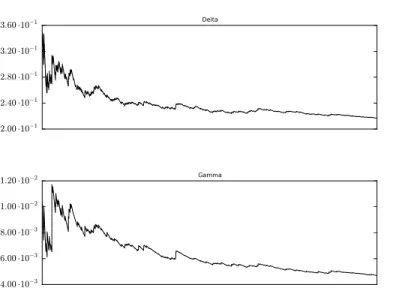
In this specific example, we will assume the Black–Scholes model. More com-plex local volatility models could be assumed. However, it would be computation-ally challenging to simulate its diffusion bridges and hence outside the scope of this paper. Below we show the convergence plots of∆xf(X0)and∆xxf(X0). These
quantities are computed using Theorems 4.8 and 4.16. Moreover, we present the
plot of the Vega of f as defined in Section 4.2.4. More precisely, we plot m(x,t)
computed by Equation 46.
Considering the parameters given in Table 1, we show the results in Table 2 and in Figures 4 and 5.
Parameter Value
Initial Value 100
Volatility 0.25
Strike(K) 100
Variance Barrier(H) 0.06
Maturity 1.0
Table 1: Parameters of the example of the VKO Call option.
Mean Standard Error
f(X0) 4.2128 0.11432
∆xf(X0) 0.2166 0.00833
∆xxf(X0) 0.00469 0.000527
2.00 ·10−1
2.40 ·10−1
2.80 ·10−1
3.20 ·10−1
3.60 ·10−1 Delta
4.00 ·10−3
6.00 ·10−3
8.00 ·10−3
1.00 ·10−2
1.20 ·10−2 Gamma
Figure 4: Convergence Plot of Monte Carlo Method to Compute ∆xf(X0) and
∆xxf(X0).
Time
0.0 0.2 0.4 0.6 0.8 1.0
Spot Value
40 60
80 100
120 140
160
Vega
−3.0 ·10−4
−2.0 ·10−4
−1.0 ·10−4
0.0 1.0 ·10−4
2.0 ·10−4
3.0 ·10−4
Figure 5: Plot of m(x,t)- the Vega for a VKO Call option. The axes Time and
4.3
More on Delta
In the following we will derive formulas for the Delta of a derivative contract dis-tinguishing each path-dependence structure presented in Definition 3.4.
The goal of this section is twofold: show how the result found in [12] using Malliavin calculus can be achieved using functional Itˆo calculus and then provide a better understanding of the assumption used in the Malliavin calculus framework
that the contractgis of the form:
g(YT) =φ(yt1, . . . ,ytn).
(48)
In short, this assumption implies that contracts of this form generate derivatives prices that are discretely monitored functionals, see Definition 3.4. The main feature of these functionals is that they exhibit weak path-dependence but for the finite set of times{t1, . . . ,tn}, see Proposition 3.6.
4.3.1 Discretely Monitored Functionals
In this section we consider a simple modification of the method described in Sec-tion 4.2 to handle discretely monitored funcSec-tionals as studied in [12], see EquaSec-tion (48).
Theorem 4.22. Assume the no-arbitrage price of a path-dependent derivative, denoted by f , is a discretely monitored functional and that f satisfy Assumptions 4.6. Hence, we find the same representation for the Delta as in [12]:
∆xf(X0) =E
g(XT) Z T
0
a(t)zt
σ(Xt)
dwt
,
(49)
for any a∈Γ, where
Γ=
a∈L2[0,T];
Z ti
0
a(t)dt =1, ∀i=1, . . . ,n
.
(50)
Proof. To focus on the essential arguments of the proof, we consider the case
with only two monitoring datest1<T. This setting allow us to introduce all the
elements of the proof without the burden of heavy notations. A similar reasoning could be applied to the general case.
As we have seen in Equation (30),
d(∆xf(Xt)zt) =−Lf(Xt)ztdt+dmt,
with(mt)t∈[0,T]being a local martingale. By well-known localization arguments,
we assume m is a martingale. As seen in Proposition 3.6, we have Lf(Xt) =0
for allt∈[0,t1)∪(t1,T]. SinceLf does not exist att =t1, we are able integrate
Equation (51) over intervals not containingt1. Fixε >0 and fort ∈(t1,T], we
integrate the SDE (51) over the interval[t1+ε,t], we get
∆xf(Xt)zt =∆xf(Xt1+ε)zt1+ε+mt−mt1+ε.
So, multiplying by anya∈Γand integrating with respect tot, we have
Z T
t1+ε
∆xf(Xt)zta(t)dt
=
Z T
t1+ε
∆xf(Xt1+ε)zt1+εa(t)dt+
Z T
t1+ε
(mt−mt1+ε)a(t)dt
=∆xf(Xt1+ε)zt1+ε
Z T
t1+ε
a(t)dt+
Z T
t1+ε
(mt−mt1+ε)a(t)dt
(52)
Fort∈[0,t1), integrating again Equation (51) now over the interval[0,t], we
get
∆xf(Xt)zt =∆xf(X0) +mt.
Multiplying bya∈Γand integrating with respect tot give us
Z t1−ε
0
∆xf(Xt)zta(t)dt
=
Z t1−ε
0
∆xf(X0)a(t)dt+
Z t1−ε
0
mta(t)dt
=∆xf(X0)
Z t1−ε
0
a(t)dt+
Z t1−ε
0
mta(t)dt
(53)
Summing the two Equations (52) and (53), taking the expectation and using
the factmis a martingale, we find
E
Z t1−ε
0 +
Z T
t1+ε
∆xf(Xt)zta(t)dt
=∆xf(X0)
Z t1−ε
0
a(t)dt+∆xf(Xt1+ε)zt1+ε
Z T
t1+ε
a(t)dt
+E
Z t1−ε
0
mta(t)dt
+E
Z T
t1+ε
(mt−mt1+ε)a(t)dt
=∆xf(X0)
Z t1−ε
0
a(t)dt+∆xf(Xt1+ε)zt1+ε
Z T
t1+ε
Therefore, the result follows lettingε →0+and applying the integration by parts
formula and using thata∈Γ, that meansRt1
0 a(t)dt =1 and
RT
t1 a(t)dt =0.
Remark 4.23. Comparing with Equation (24), we conclude that Theorem 4.22 gives the same weight as in [12].
Remark 4.24. Consider a contractg(XT) =φ(xt1, . . . ,xtn), where 0<t1<· · ·<
tn≤T are fixed times andφ :Rn−→R. In the case of local volatility models, the
assumption that f is a discretely monitored functional in the previous Theorem is
automatically satisfied as one can simply deduce from
f(Yt) =E[φ(xt1, . . . ,xtn)|Yt],
and from Definition 3.4.
We would like to conclude this section observing that we were able to de-rive, using the techniques of the functional Itˆo calculus, the same results of [12], in which Malliavin calculus was used. Furthermore, the method implemented here enlightens the assumption that the derivative price needs to be a discretely monitored functional to employ Theorem 4.22. Indeed, the main feature of such functionals is that it is weakly path-dependent in the interval(ti,ti+1)allowing us
to apply the integration by parts formula in each of these interval.
4.3.2 Delayed Path-Dependent Functionals
The argument presented in the proof of Theorem 4.22 can be generalized to the delayed path-dependent functionals. The next proposition states precisely the re-sult.
Define
Γs=
a∈L2([0,T]);
Z s
0
a(t)dt =1 anda(t) =0, fort≥s
.
Proposition 4.25. Fix a t1-delayed path-dependent functional f satisfying As-sumptions 4.6 and consider a∈Γt1. Thus,
∆xf(X0) =E
g(XT) Z t1
0
a(t)zt
σ(Xt)
dwt
.