350
MAXIMUM LIKELIHOOD PARAMETER ESTIMATORS
FOR THE TWO POPULATIONS GEV DISTRIBUTION
Jose A. Raynal-Villasenor
Department of Civil and Environmental Engineering
Universidad de las Americas, Puebla, 72820 Cholula, Puebla, Mexico
ABSTRACT
The method of maximum likelihood for estimating the parameters of the two populations general extreme value (TPGEV) probability distribution function for the maxima is presented for the case of flood frequency analysis. The proposed methodology is compared with widely used models, namely: two component extreme value (TCEV), general extreme value (GEV) and Gumbel distributions. The TPGEV distribution behaved well for those selected sets of data in Northwestern Mexico and the results of this distribution proved to be better than the TCEV model, when there are two populations present in the flood sample of data. The paper contains several numerical examples of the application of the proposed methodology.
Keywords: probability, flood frequency analysis, maximum likelihood, parameter estimation, mixed distributions
1. INTRODUCTION
The method of maximum likelihood has been acknowledged as one of the best methods for parameter estimation of probability distribution functions. The properties of its estimators like the invariance property, Mood et al [1], and the asymptotically unbiasedness, sufficiency, for a particular class of probability distribution functions, consistency and efficiency, (Haan [2]) and the remarkable suitability when being applied to cumbersome mathematical expressions in its likelihood functions under some strict regularity conditions, have gained it the well-known condition of prime choice for solving problems of parameter estimation of probability distribution functions.
The use of the general extreme value (GEV) distribution function (Jenkinson [3], [4]) for flood frequency analysis is widespread enough and it is now a feasible option, by the practicing engineers, for application in the flood frequency analysis process (NERC [5]; Prescott and Walden [6]; and Hosking [7]).The use of a mixture of probability distributions functions for modeling samples of data coming from two populations have been proposed long time ago (Mood et al [1]). In the particular case of extreme value distributions, several options have been proposed so far, the TCEV distribution (Gumbel [8]; Todorovic and Rousselle [9]; Canfield [10]; and Rossi et al [11]) the mixed Gumbel distribution, (Gonzalez-Villarreal [12]; Raynal-Villasenor [13]; and Raynal-Villasenor and Guevara-Miranda [14]), and the mixed general extreme value distribution (Raynal-Villasenor and Santillan-Hernandez [15]; and Gutierrez-Ojeda and Raynal-Villasenor [16]).
It is the purpose of this paper to expand the knowledge of the two populations general extreme value distribution in the case of the maxima, by providing the procedure of application of the method of maximum likelihood for estimating its parameters.
2. THE GENERAL EXTREME VALUE DISTRIBUTION FOR THE MAXIMA The probability distribution function of the GEV distribution for the maxima is, NERC [5]:
F
(
x
)
exp
1
(
x
)
1 /
(1)where , , and are the scale, shape and location parameters. The probability density function is given by, NERC [5]:
1 / 1 /
1
)
(
1
)
(
1
exp
1
)
(
x
x
x
f
(2)For extreme value type I (Gumbel) distribution ( 0; = 1.1396):
351
+ / x < (4) For extreme value type III (Weibull) distribution ( > 0; < 1.1396):
- < x + / (5) where is the coefficient of skewness.
3. THE TWO POPULATIONS GENERAL EXTREME VALUE DISTRIBUTION
Based in the general form for two populations probability distributions functions (Mood et al [1]):
)
;
(
)
;
(
)
1
(
)
(
x
p
F
x
1pF
x
2F
mix
(6)where p is the proportion of the second population in the mixture. The TPGEV distribution can be constructed as:
2 1 1 / 1 2 2 2 / 1 11
(
)
1
exp
)
(
1
exp
)
1
(
)
(
x
p
x
p
x
F
mix (7) and the corresponding probability density function is:
11 1/
1 1 1 1 / 1 1 1 1 1
)
(
1
exp
(
1
)
1
(
)
(
x
x
p
x
f
mix
22 1/
2 2 2 1 / 1 2 2 2 2
)
(
1
exp
)
(
1
x
x
p
(8)4. THE METHOD OF MAXIMUM LIKELIHOOD
The method of maximum likelihood have been defined and applied to several probability distribution functions with defined probability density functions (pdf) (NERC [5]). Such method has suitable characteristics like the invariance property (Mood et al [1]), and the asymptotically unbiasedness, sufficiency, consistency and efficiency (Haan [2]) in large sample estimation and applicability in estimating the parameters of complex probability density functions. The likelihood function of N independent random variables is defined to be the joint probability density function of N random variables and is viewed as a function of the parameters. If X1 , ..., XN is a random sample of a
univariate probability density function, the corresponding likelihood function for the observed X1 , ..., XN sample
is (Mood et al [1]):
N i ix
f
x
L
1)
(
)
,
(
(9)where denotes the parameter set and f(.) is the probability density function. The logarithmic version of eq. (8) is:
)]
(
[
)]
,
(
[
1 i N ix
f
Ln
x
L
Ln
(10)and will be used instead of the former equation because it is easier to handle in the computational procedure described in the next section.
The set of parameters that maximize equation (9), if they exists, will be the maximum likelihood estimators for the parameters of the probability distribution function.
5. MAXIMUM LIKELIHOOD PARAMETER ESTIMATORS FOR THE TWO POPULATIONS GEV
DISTRIBUTION FOR THE MAXIMA
Based in the principles contained in the previous section, the log-likelihood function for the TPGEV distribution for the maxima is:
352
2 21 1/
2 2 2 1 / 1 2 2 2 2 1 / 1 1 1
1
(
)
1
exp
)
(
1
)
(
1
exp
i ii
p
x
x
x
(11)
and the corresponding first order partial derivatives of such function with respect to each of the parameters are:
N i j j j i j i j j j i j i j j jDEN
x
x
F
x
x
F
C
L
Ln
j j 1 2 / 1 2 / 2 2)
(
1
)
;
(
)
(
1
)
;
(
)
(
(12) j = 1, 21 / 1 1 2
)
(
1
)
;
(
)
(
j j j j i j i N i j j jx
x
F
C
L
Ln
DEN
x
x
x
x
f
j j j j i j j j i j j i j i
1 / 1)
(
1
)
(
1
/
)
1
(
)
)(
;
(
(13) j = 1, 2
N i j j j i j j i j j j j i j j j j i j j jDEN
x
x
x
Ln
x
C
L
Ln
j 1 2 / 1)
(
1
)
)(
1
(
)
(
1
1
)
(
1
exp
)
(
(14) j = 1, 2
N iDEN
x
f
x
f
p
L
Ln
1 2 1)
(
;
)
353
mix
x
f
DEN
(
)
(16)
1
/ 1 1 1
1 1
)
(
1
exp
)
;
(
x
x
F
(17)
2
/ 1 2 2
2 2
)
(
1
exp
)
;
(
x
x
F
(18)C1 = 1-p ; C2 = p (19)
The exact solution provided by the system of equations (12)-(14) is not known for the case of the of TPGEV distribution, so the maximum likelihood estimators of the parameters of the TPGEV distribution may be obtained by either solving numerically, e.g. by the method of Newton, the system of non-linear equations ( equations (12)-(14)), or by a direct maximization of the log-likelihood function, equation (11), by a non-linear optimization procedure, e.g. the multivariable constrained Rosenbrock method (Kuester and Mize [17]). In this study the former option was the choice for estimating the parameters of the TPGEV distribution by the method of maximum likelihood.
6. THE TCEV DISTRIBUTION
The Two Component Extreme Value probability distribution has been defined (Rossi et al [11]) as:
2 2
1
1
exp
exp
exp
)
(
x
x
x
F
(20)where i is thelocation parameter and θi is the shape parameter of the TCEV distribution.
The maximum likelihood parameters of the TCEV distribution are obtained by an iterative scheme using the following equations (Rossi et al [11]):
N
i j
i j
N
i i
i
j
j
x
x
x
1 1
1
exp
)
(
exp
; j = 1, 2 (21)
N
i
N
i i
j i
j i i
i N
i j
i i
j
x
x
x
x
x
x
x
1 1
1
)
(
exp
exp
)
(
exp
; j = 1, 2 (22)where ψ(.) is the digamma function with argument (.).
7. RESULTS AND DISCUSSION
354
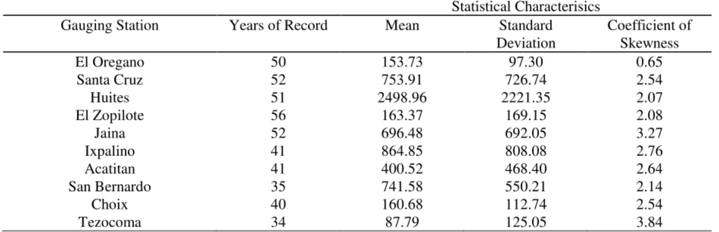
estimators of the parameters of the TPGEV distribution were computed. Those gauging stations are located in an area that every year is affected by tropical cyclones, during summer and fall, and cold fronts, during winter, causing the presence of at least two populations in the samples of flood data. The years of record, computed sample mean, standard deviation and coefficient of skewness of the samples of flood data for the selected gauging stations are shown in table 1.
Table 1. Statistical characteristics of flood data of the selected gauging stations Statistical Characterisics
Gauging Station Years of Record Mean Standard
Deviation
Coefficient of Skewness
El Oregano 50 153.73 97.30 0.65
Santa Cruz 52 753.91 726.74 2.54
Huites 51 2498.96 2221.35 2.07
El Zopilote 56 163.37 169.15 2.08
Jaina 52 696.48 692.05 3.27
Ixpalino 41 864.85 808.08 2.76
Acatitan 41 400.52 468.40 2.64
San Bernardo 35 741.58 550.21 2.14
Choix 40 160.68 112.74 2.54
Tezocoma 34 87.79 125.05 3.84
The one population general extreme value and Gumbel distributions computed parameters, were obtained through the application of user-friendly computer package FLODRO 4.0 (Raynal-Villasenor [18]) for the selected gauging stations, and they are shown in tables 2 and 3.
The TPGEV and TCEV distribution computed parameters for such gauging stations were evaluated by using computer code FLODRO 4.0 (Raynal-Villasenor [18]) and the results are contained in tables 4 and 5.
In order to compare the results provided by the TPGEV distribution with those produced by other widely applied models, such the one population general extreme value (GEV), Gumbel (G) and Two Component Extreme Value (TCEV) distributions, in table 6 a compilation is presented of the design values for several return periods and their standard errors of fitting, EE, produced by the methods mentioned above and the one proposed in the paper. The EE is defined as (Kite [19]):
2 / 1 2 1
)
(
)
(
j i i N
i
m
N
y
x
EE
(23)where xi are the historical values of the sample, yi are the values produced by the distribution function corresponding to the same return periods of the historical values, N is the sample size, and mj is the number of parameters of the distribution function.
Table 2. One population GEV and Gumbel (EV-I) distributions parameters for the selected gauging stations
Gumbel Parameters
GEV Parameters
Gauging Station λ λ
El Oregano 108.84 95.98 109.43 77.05 0.016
Santa Cruz 567.28 426.88 406.89 349.47 -0.320
Huites 1650.26 1212.08 1402.62 874.92 -0.455
El Zopilote 97.05 100.98 78.34 80.35 -0.372
Jaina 451.58 361.29 386.64 284.05 -0.357
Ixpalino 572.42 436.54 510.07 370.85 -0.275
Acatitan 241.58 241.34 194.24 181.28 -0.407
San Bernardo 527.17 325.54 476.43 272.37 -0.305
Choix 109.28 73.92 104.97 71.14 -0.107
355
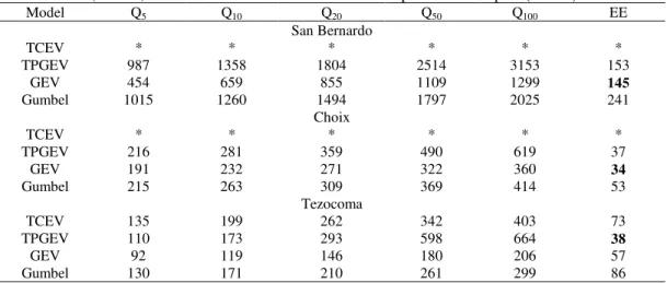
The results of this study provide the arguments to establish the following points:
1) The TPGEV distribution function behaved very well in the selected gauging stations, just in two out of ten it cannot reach convergence. The TCEV failed to attain convergence in three samples of flood data. In the case of the TPGVE, the lack of convergence was not solved by changing the initial values in the optimization procedure, it seems that for a specific sample of flood data the procedure just will have a lack of convergence, so in those cases such model simply won´t work. The lack of convergence in the case of the TCEV it seems is associated by the estimation procedure itself, it won´t converge in many instances. 2) The TPGEV distribution function has the least standard error of fit (EE) in five gauging stations and was
very close to the least value in four additional gauging stations. The GEV reached the least value of the EE in five of the gauging stations
3) None of the Gumbel (extreme value type I) nor the TCEV distributions were even close to any of the least values of the EE in the ten selected gauging stations
4) The TPGEV distribution function has the least standard error of fit (EE) in five gauging stations and was very close to the least value in three additional gauging stations. The GEV reached the least value of the EE in five of the gauging stations
5) With regard to the design values, for those gauging stations where the TPGEV distribution produced the best fit, the produced values were much higher than those for the GEV distribution
6) The computation of the parameters and design values for the TPGEV distribution were made possible by the use of a personal computer. It will be very difficult, if not impossible, to evaluate such parameters and design values with a portable calculator or some other computing device with less capacity than a personal computer. This is a drawback that the proposed method has and there is no way to overcome it, given the enormous number of calculations that the optimization code has to perform in order to obtain the maximum likelihood estimators of the parameters of the TPGVE distribution
8. CONCLUSIONS
The procedure of finding the estimators of the parameters of the TPGEV distribution for the maxima, using the method of maximum likelihood, has been presented.
The TPGEV distribution behaved well for those selected sets of flood data, just in two out of the ten cases considered for analysis, the TPGEV could not reach convergence in the estimation of parameters process. The lack of convergence was not solved by changing the initial values in the optimization procedure, it seems that for a specific sample of flood data the procedure just will have a lack of convergence, so in those cases such model simply won´t work. In these cases another model of mixed distributions should be used.
The TCEV had three failures in the estimation of the parameters process due to the lack of convergence. The lack of convergence in the case of the TCEV it seems is associated by the estimation procedure itself, it won´t converge in many instances.
In five cases the TPGEV distribution produced the least standard error of fit and in other three cases was very close to the GEV distribution which has the least standard error of fit in such samples of flood data.
It will be wise to consider the presence of two populations in the sample of flood data, in addition to the standard error of fit, to reach a decision on which model to use for flood frequency analysis.
Table 3. TPGEV distribution parameters for the selected gauging stations
Station λ1 1 1 λ2 2 2 p
El Oregano 67.47 41.42 9.6 10-6 195.54 67.31 -0.01 0.441
Santa Cruz * * * * * * *
Huites 1194.05 506.37 0.068 3389.28 2034.51 -0.082 0.309
El Zopilote * * * * * * *
Jaina 259.02 146.21 0.0131 632.19 395.34 -0.269 0.541
Ixpalino 445.49 190.14 1.020 583.68 444.93 -0.266 0.755
Acatitan 241.71 74.48 0.704 188.29 206.94 -0.597 0.731
San Bernardo 413.44 190.27 5.4 10-4 699.78 413.00 -0.233 0.422
Choix 85.86 24.85 0.535 178.29 54.13 -0.347 0.483
Tezocoma 36.53 34.15 -0.3050 553.31 163.70 1.1448 0.033
356
Table 4. TCEV distribution parameters for the selected gauging stations
Station 1 1 2 2 p
El Oregano 6.75 11.26 3.32 80.47 0.330
Santa Cruz 4.20 62.01 2.47 506.96 0.369
Huites * * * * *
El Zopilote 2.33 10.60 2.02 125.07 0.465
Jaina 5.12 115.18 1.69 490.28 0.248
Ixpalino 3.35 198.30 1.75 563.66 0.550
Acatitan 2.29 77.71 1.50 309.42 0.396
San Bernardo * * * * *
Choix * * * * *
Tezocoma 2.54 17.06 1.05 86.64 0.292
* No convergence was attained
Based in the results presented in the paper, the author recommend this procedure to be included in the standard methods for flood frequency analysis, as an additional model for the flood frequency analysis when there is the possibility that two populations are present in the samples of flood data.
Table 5. Comparison of Design Values (in m3/s) and Standard Errors of Fitting (in m3/s) Between Several Models for One and Two Populations Samples
Model Q5 Q10 Q20 Q50 Q100 EE
El Oregano
TCEV 217 278 336 411 467 17
TPGEV 234 290 341 406 455 10
GEV 225 283 338 410 464 14
Gumbel 223 280 335 405 458 14
Sta. Cruz
TCEV 1218 1599 1964 2436 2790 275
TPGEV * * * * * *
GEV 1102 1413 1714 2105 2398 161
Gumbel 1112 1430 1736 2131 2427 321
Huites
TCEV * * * * * *
TPGEV 3153 5557 8451 9641 9938 260
GEV 2724 3385 4020 4842 5457 541
Gumbel 3468 4377 5250 6380 7226 1046
Zopilote
TCEV 256 340 421 525 604 62
TPGEV * * * * * *
GEV 199 259 317 392 448 30
Gumbel 248 324 397 491 562 69
Jaina
TCEV 995 1361 1714 2170 2513 324
TPGEV 981 1416 1916 2714 2453 245
GVE 813 1026 1230 1425 1693 224
Gumbel 993 1264 1524 1861 2114 372
Ixpalino
TCEV 1183 1591 1992 2516 2909 397
TPGEV 1199 1722 2324 3290 4186 267
GEV 1066 1345 1612 1957 2216 285
Gumbel 1227 1555 1869 2276 2581 416
Acatitan
TCEV 592 823 1045 1334 1550 227
TPGEV 527 930 1525 2787 4314 48
GEV 466 602 732 902 1028 135
Gumbel 595 776 951 1176 1345 251
TCEV = Two Component Extreme Value Distribution
357
Table 5. Comparison of Design Values (in m3/s) and Standard Errors of Fitting (in m3/s) Between Several Models for Two Populations Samples (cont’d)
Model Q5 Q10 Q20 Q50 Q100 EE
San Bernardo
TCEV * * * * * *
TPGEV 987 1358 1804 2514 3153 153
GEV 454 659 855 1109 1299 145
Gumbel 1015 1260 1494 1797 2025 241
Choix
TCEV * * * * * *
TPGEV 216 281 359 490 619 37
GEV 191 232 271 322 360 34
Gumbel 215 263 309 369 414 53
Tezocoma
TCEV 135 199 262 342 403 73
TPGEV 110 173 293 598 664 38
GEV 92 119 146 180 206 57
Gumbel 130 171 210 261 299 86
TCEV = Two Component Extreme Value Distribution
TPGEV = Two Populations General Extreme Value Distribution * No convergence was attained in the estimation of parameters process Bold numbers correspond to the distribution with best fit
9. ACKNOWLEDGEMENTS
The author wish to express their gratitude to the Universidad de las Americas, Puebla for the support provided in the realization of this paper.
10. REFERENCES
[1]. Mood, A. M., Graybill, F. and Boes, D. C. Introduction to the Theory of Statistics, McGraw-Hill Inc., Third Ed., New York, N. Y., 276-286. (1974).
[2]. Haan, C.T. Statistical Methods in Hydrology, The Iowa State University Press, Ames, Iowa, 63. (1977).
[3]. Jenkinson, A. F. The Frequency Distribution of the Annual, Maximum (or Minimum) Values of Meteorological Elements, Quart. J. Royal Met. Soc., 87, 158-171. (1955).
[4]. Jenkinson, A. F. Estimation of Maximum Floods, Chapter 5, WMO, Technical Note 98, Geneva, Switzerland, 183-227. (1969).
[5]. Natural Environment Research Council, (NERC) Flood Studies Report, I, Hydrologic Studies, Whitefriars Press Ltd., London, 51. (1975).
[6]. Prescott, P. and Walden, A. T. Maximum Likelihood Estimation of the Parameters of the Generalized Extreme Value Distribution, Biometrika, 67(3), 723-724. (1980).
[7]. Hosking, J. R. M. L-moments: Analysis and Estimation of Distribution using Linear Combination of Order Statistics, J. R. Statist. Soc. B, 52, No. 1, 105-124. (1990).
[8]. Gumbel, E. J. Statistics of Extremes, Columbia University Press, New York, N. Y., 8. (1958).
[9]. Todorovic, P. and Rousselle, J. Some Problems of Flood Analysis, Wat. Resour. Res., 7(5), 1144-1150. (1971)
[10]. Canfield, R. V. The Distribution of the Extremes of a Mixture of Random Variable with Applications to Hydrology, in Input for Risk Analysis in Water Systems, E.A. McBean, K. W. Hipel and T. E. Unny, eds., Water Resources Publications, 77-84. (1979).
[11]. Rossi, F., Florentino, M. and Versace, P. Two Component Extreme Value Distribution for Flood Frequency Analysis, Wat. Resour. Res., 20(7), 847-856. (1984).
[12]. Gonzalez-Villareal, F. J. Contribution to the Frequency Analysis of the Extreme Values of the Floods in a River, Report # 277, Instituto de Ingenieria, Universidad Nacional Autonoma de Mexico, Mexico, D.F., Mex. (in Spanish) (1970). [13]. Raynal-Villasenor, J.A. Maximum Likelihood Estimators of the Parameters of the Mixed Gumbel Distribution, XII
Congress of the National Academy of Engineering, Saltillo, Coah., Mex., 468-471. (in Spanish) (1986).
[14]. Raynal-Villasenor, J. A. and Guevara-Miranda, J. L. Maximum Likelihood Estimators for the Two Populations Gumbel Distribution, Hydrological Science and Technology J., Vol. 13, No. 1-4, pp 47-56. (1997).
[15]. Raynal-Villasenor, J. A., and Santillan-Hernandez, O. D. Maximum Likelihood Estimators of the Parameters of the Mixed General Extreme Value Distribution, IX National Congress on Hydraulics, Queretaro, Qro., Mex., National Association of Hydraulics, 79-90. (In Spanish) (1986).
[16]. Gutierrez-Ojeda, C. and Raynal-Villasenor, J. A. Mixed Distributions in Flood Frequency Analysis, X National Congress on Hydraulics, Morelia, Mich., Mex., National Association of Hydraulics, 220-228. (in Spanish) (1988). [17]. Kuester, J. L. and Mize, J. H. Optimization Techniques with FORTRAN, Mc-Graw Hill Book Co., 386-398. (1973). [18]. Raynal-Villasenor J. A. Frequency Analysis of Hydrologic Extremes, Lulu.com, USA. (2010).