www.the-cryosphere.net/4/285/2010/ doi:10.5194/tc-4-285-2010
© Author(s) 2010. CC Attribution 3.0 License.
The Cryosphere
Manufactured analytical solutions for isothermal full-Stokes ice
sheet models
A. Sargent and J. L. Fastook
Climate Change Institute, University of Maine, Orono, USA
Received: 25 March 2010 – Published in The Cryosphere Discuss.: 8 April 2010 Revised: 16 July 2010 – Accepted: 27 July 2010 – Published: 18 August 2010
Abstract. We present the detailed construction of a man-ufactured analytical solution to time-dependent and steady-state isothermal full-Stokes ice sheet problems. The solu-tions are constructed for two-dimensional flowline and three-dimensional full-Stokes ice sheet models with variable vis-cosity. The construction is done by choosing for the speci-fied ice surface and bed a velocity distribution that satisfies both mass conservation and the kinematic boundary condi-tions. Then a compensatory stress term in the conservation of momentum equations and their boundary conditions is cal-culated to make the chosen velocity distributions as well as the chosen pressure field into exact solutions. By substitut-ing different ice surface and bed geometry formulas into the derived solution formulas, analytical solutions for different geometries can be constructed.
The boundary conditions can be specified as essential Dirichlet conditions or as periodic boundary conditions. By changing a parameter value, the analytical solutions allow investigation of algorithms for a different range of aspect ra-tios as well as for different, frozen or sliding, basal condi-tions. The analytical solutions can also be used to estimate the numerical error of the method in the case when the ef-fects of the boundary conditions are eliminated, that is, when the exact solution values are specified as inflow and outflow boundary conditions.
1 Introduction
Model verification is crucial in developing a numerical model. The ice-sheet modeling community has been using two tools to verify models, comparison of numerically com-puted solutions to analytical solutions when possible, and in-tercomparison, that is, measuring differences between vari-ous models’ results on the sets of simplified geometry bench-mark tests.
computing the three-dimensional stress and velocity field in grounded glaciers in (Blatter, 1995). Analytical so-lutions have been found describing transient two dimen-sional flow (Hutter, 1980, 1983; Johannesson, 1992; Bahr, 1996), three-dimensional steady-state flow (Reeh, 1987; Jo-hannesson, 1992) and transient evolution flow (Gudmunds-son, 2003).
All the above solutions give physical insight into the flow processes; however, they cannot be easily used to bench-mark the numerical solutions. For example, Gudmundsson in (Gudmundsson, 2003) obtained the three-dimensional so-lution of the linearized zeroth-order problem for a linear vis-cous medium. To use this solution for benchmarking nu-merical ice sheet models, the exact error estimate must be known (Raymond and Gudmundsson, 2005).
In this paper, we present the detailed construction of a manufactured exact solution to time-dependent and steady-state isothermal full-Stokes ice sheet problems. The solu-tions are constructed for three-dimensional (3-D) full-Stokes and two-dimensional (2-D) flowline ice sheet models with variable viscosity. The construction is done by choosing for the specified ice surface and bed the velocity distributions that satisfy the mass conservation equation and the kinematic boundary conditions, and by then calculating the required force distribution that makes the chosen velocities and pres-sure into exact solutions of the conservation of momentum equation and its boundary conditions. In the appendices we give the formulas that can be used to calculate the compen-satory stress terms for the momentum equation in the 2-D and 3-D full-Stokes models and supplement to the manuscript contains a fortran 77 code to calculate stress terms for the 2-D model.
The steady-state solutions constructed in this paper are variations of the benchmark experiments A and B in (Pattyn et al., 2008). However, by substituting different ice surface and bed geometry into the derived formulas, analytical solu-tions for different geometries can also be constructed.
The boundary conditions can be specified as essential Dirichlet conditions or as periodic boundary conditions. By changing a parameter value, the analytical solutions allow modelers to investigate their solutions for a range of aspect ratios as well as for different, frozen or sliding, basal condi-tions. Finally, the analytical solutions may help the model-ers to estimate the numerical error in the case when the ef-fect of the boundary conditions are eliminated, that is, when the exact solutions values are specified as inflow and outflow boundary conditions.
2 Model physics 2.1 Model equations
We consider an ice sheet model in the Cartesian coordinates ˜
x=(x,˜ y,˜ z)˜ with the domain 0≤ ˜x≤L, 0≤ ˜y≤L,b(˜ x,˜ y)˜ ≤ ˜
z≤ ˜s(x,˜ y,˜ t )˜, wheret˜is time, s(˜ x,˜ y,˜ t )˜ defines the surface andb(˜ x,˜ y)˜ defines the base of the glacier.
Bed elevationb(˜ x,˜ y)˜ and accumulation ratea˜˙ are time in-dependent, while surface elevations(˜ x,˜ y,˜ t )˜ can change with time. The solution is the velocity vectorv˜=(u,˜ v,˜ w)˜ and ice pressurep˜. Dimensional variables in this work are denoted with a tilde and non-dimensional variables without.
The field equations for the isothermal ice sheet model con-sist of the conservation of mass and the conservation of mo-mentum:
∂u˜ ∂x˜+
∂v˜ ∂y˜+
∂w˜
∂z˜ =0, (1)
∂2µ˜∂∂ux˜˜+ ˜p
∂x˜ +
∂µ˜∂∂yu˜˜+∂∂vx˜˜
∂y˜ +
∂µ˜∂∂uz˜˜+∂∂wx˜˜
∂z˜ =0, (2)
∂
˜ µ
∂u˜
∂y˜+∂
˜ v
∂x˜
∂x˜ +
∂
2µ˜∂∂vy˜˜+ ˜p
∂y˜ +
∂
˜ µ
∂v˜
∂˜z+∂
˜ w
∂y˜
∂z˜ =0, (3)
∂µ˜∂∂wx˜˜+∂∂uz˜˜ ∂x˜ +
∂µ˜∂∂wy˜˜ +∂∂vz˜˜ ∂y˜ +
∂2µ˜∂∂wz˜˜+ ˜p
∂z˜ = ˜ρg,˜ (4) whereρ˜is the ice density,g˜is the gravitational acceleration,
˜
µis the effective viscosity
˜ µ=B
2 "
1 4
∂u˜ ∂y˜+
∂v˜ ∂x˜
2 +1
4
∂u˜ ∂z˜+
∂w˜ ∂x˜
2 +1
4
∂v˜ ∂z˜+
∂w˜ ∂y˜
2 (5)
−∂u˜ ∂x˜
∂v˜ ∂y˜−
∂u˜ ∂x˜
∂w˜ ∂z˜ −
∂v˜ ∂y˜
∂w˜ ∂z˜
1−2nn ,
Bis a temperature-independent rate factor, andnis the stress exponent.
2.2 Boundary conditions
The model is time-dependent in the usual sense that the ice sheet geometry evolves according to a mass continuity equation. We assume that the ice has a hard bed, ∂b∂t =0. The kinematic boundary conditions applied at the upper and lower surfaces of the ice mass are as follows:
∂s˜
∂t˜+ ˜u(x,˜ y,˜ s,˜ t )˜ ∂s˜
∂x˜+ ˜v(x,˜ y,˜ s,˜ t )˜ ∂s˜
∂y˜− ˜w(x,˜ y,˜ s,˜ t )˜ = ˙˜a,
˜
u(x,˜ y,˜ b,˜ t )˜ ∂b˜
∂x˜+ ˜v(x,˜ y,˜ b,˜ t )˜ ∂b˜
The stress-free boundary conditions at the upper surface
˜
s(x,˜ y,˜ t )˜ are defined as:
1
˜
rs
−∂s˜
∂x˜
2µ˜∂u˜
∂x˜+ ˜p
−∂s˜
∂y˜µ˜ ∂u˜
∂y˜+
∂v˜
∂x˜
+ ˜µ
∂u˜
∂z˜+
∂w˜
∂x˜
=0,
1
˜
rs
−∂s˜
∂x˜µ˜ ∂u˜
∂y˜+
∂v˜
∂x˜
−∂s˜
∂y˜
2µ˜∂v˜
∂y˜+ ˜p
+ ˜µ
∂v˜
∂˜z+ ∂w˜
∂y˜
=0,
1
˜
rs
−∂s˜
∂x˜
˜
µ
∂w˜
∂x˜+
∂u˜
∂˜z
−∂s˜
∂y˜
˜
µ
∂w˜
∂y˜+
∂v˜
∂˜z
+
2µ˜∂w˜
∂z˜+ ˜p
=0,
wherer˜s=
r
1+∂∂xs˜˜2+∂∂y˜s˜2.
For the frozen-based grounded ice, the boundary condi-tions at the bedb(˜ x,˜ y)˜ can be specified as Dirichlet condi-tions:
˜
u(x,˜ y,˜ b,˜ t )˜ =0, ˜
v(x,˜ y,˜ b,˜ t )˜ =0, ˜
w(x,˜ y,˜ b,˜ t )˜ =0, ˜
p(x,˜ y,˜ b,˜ t )˜ = ˜ρg(˜ s˜− ˜b).
For the ice with sliding bed, the shear stresses may be speci-fied at the bedb(˜ x,˜ y)˜ as Robin conditions:
1
˜ rb
" ∂b˜ ∂x˜
2µ˜∂u˜
∂x˜+ ˜p
+∂b˜ ∂y˜µ˜
∂ ˜ u ∂y˜+
∂v˜ ∂x˜
− ˜µ
∂ ˜ u ∂z˜+
∂w˜ ∂x˜
= − ˜β2u(˜ x,˜ y,˜ b,˜ t ),˜
1
˜ rb
" ∂b˜ ∂x˜µ˜
∂u˜ ∂y˜+
∂v˜ ∂x˜
+∂b˜
∂y˜
2µ˜∂v˜ ∂y˜+ ˜p
− ˜µ
∂v˜ ∂z˜+
∂w˜ ∂y˜
#
= − ˜β2v(˜ x,˜ y,˜ b,˜ t ),˜
1 ˜ rb
" ∂b˜ ∂x˜
˜ µ
∂w˜ ∂x˜ +
∂u˜ ∂z˜
+∂b˜
∂y˜
˜ µ
∂w˜ ∂y˜ +
∂v˜ ∂z˜
−
2µ˜∂w˜ ∂z˜ + ˜p
#
= ˜ρg˜h,˜
wherer˜b=
r
1+∂∂xb˜˜
2
+∂∂by˜˜
2
andβ˜2is the friction coef-ficient.
Along the glacier’s upstream and downstream boundaries,
Dirichlet boundary conditions for velocities are specified along both upstream and downstream boundaries
˜
f (i,y,˜ z)˜ = ˜fexact(i,y,˜ z), i˜ =0,L;
˜
f (x,j,˜ z)˜ = ˜fexact(x,j,˜ z), j˜ =0,L;
wheref˜= ˜u,v,˜ w.˜
Here we assume that functionsf˜exactare known.
Dirichlet boundary conditions for pressure may be speci-fied along either upstream or downstream boundaries:
˜
p(0,y,˜ z)˜ = ˜pexact(0,y,˜ z),˜ orp(L,˜ y,˜ z)˜ = ˜pexact(L,y,˜ z)˜ ;
˜
p(x,˜ 0,z)˜ = ˜pexact(x,˜ 0,z),˜ or p(˜ x,L,˜ z)˜ = ˜pexact(x,L,˜ z).˜
2.3 Dimensionless equations
To non-dimensionalize variables, we choose the following typical values: Z– the mean thickness of the ice-sheet,L– the length of ice-sheet,U– a typical velocity in the horizon-tal direction,W – a typical velocity in the vertical direction, P – the mean pressure,A– the mean accumulation/ablation rate, and introduce the following non-dimensional variables (variables without tilde):
˜
z=Zz,s˜=Zs,b˜=Zb,
˜
x=Lx,y˜=Ly,
˜
u=U u,v˜=U v, (6)
˜ w=W w,
˜ p=Pp, ˜ t=T t, ˙˜ a=Aa,˙
˜ µ=B
2 U
L 1−nn
µ.
To further simplify the equations, we introduce the aspect ratio parameterδ:
δ=Z
L (7)
and require that scale factors L, U, W, and P satisfy the following relationships: B 2 U L n1
= ˜ρgZ˜ =P , W L
U Z=1, (8)
δ∂ 2µ
∂u ∂x+p
∂x +δ
∂µ∂u∂y+∂x∂v
∂y +
∂µ1δ∂u∂z+δ∂w∂x
∂z =0, (10)
δ
∂µ∂u∂y+∂v∂x
∂y +δ
∂2µ∂v∂y+p
∂x +
∂µ1δ∂v∂z+δ∂w∂y
∂z =0, (11)
δ
∂µδ∂w∂x+1δ∂u∂z
∂x +δ
∂µδ∂w∂y +1δ∂v∂z
∂y +
∂2µ∂w∂z +p
∂z −1=0, (12)
where µ= " 1 4 ∂u ∂y+ ∂v ∂x 2 +1 4 1 δ ∂u ∂z+δ
∂w ∂x 2 +1 4 1 δ ∂v ∂z+δ
∂w ∂y 2 −∂u ∂x ∂v ∂y− ∂u ∂x ∂w ∂z − ∂v ∂y ∂w ∂z
1−2nn .
The kinematic boundary conditions are invariant under the chosen set of scalings: ∂s
∂t+ u(x,y,s(x,y,t ),t) ∂s
∂x+v(x,y,s(x,y,t ),t ) ∂s
∂y−w(x,y,s(x,y,t ),t )= ˙a, (13)
u(x,y,b(x,y),t )∂b
∂x+v(x,y,b(x,y),t ) ∂b
∂y−w(x,y,b(x,y),t )=0. (14)
The stress-free boundary conditions at the upper surfaces(x,y,t )become as follows: 1
rs
−δ∂s
∂x
2µ∂u ∂x+p
−δ∂s
∂yµ ∂u ∂y+ ∂v ∂x +µ 1 δ ∂u ∂z+δ
∂w ∂x
=0, (15)
1 rs
−δ∂s
∂xµ ∂u ∂y+ ∂v ∂x −δ∂s
∂y
2µ∂v ∂y+p
+µ 1 δ ∂v ∂z+δ
∂w ∂y
=0, (16)
1 rs
−δ∂s
∂x µ δ∂w ∂x+ 1 δ ∂u ∂z −δ∂s
∂y µ δ∂w ∂y + 1 δ ∂v ∂z + 2µ∂w
∂z +p
=0, (17)
wherers=
r
1+δ2 ∂s ∂x
2
+δ2∂s ∂y
2 .
The Robin boundary conditions at the lower surfaceb(x,y)become as follows: 1 rb δ∂b ∂x
2µ∂u ∂x+p
+δ∂b
∂yµ ∂u ∂y+ ∂v ∂x −µ 1 δ ∂u ∂z+δ
∂w ∂x
= −β2u, (18)
1 rb δ∂b ∂xµ ∂u ∂y+ ∂v ∂x +δ∂b
∂y
2µ∂v ∂y+p
−µ
1 δ
∂v ∂z+δ
∂w ∂y
= −β2v, (19)
1 rb δ∂b ∂x µ δ∂w ∂x + 1 δ ∂u ∂z +δ∂b
∂y µ δ∂w ∂y + 1 δ ∂v ∂z − 2µ∂w
∂z +p
=1, (20)
whererb=
r
1+δ2 ∂b ∂x
2
+δ2∂b ∂y
2 .
3 Manufactured analytical solutions of the 2-D full-Stokes isothermal flowline ice sheet model 3.1 Deriving an exact solution
Two-dimensional full-Stokes flowline models have only one horizontal dimension,x. So all terms in the Eqs. (10–20) that have variablesyorv, as well as all partialy−derivatives of velocities and pressure can be removed.
To satisfy the 2-D version of the kinematic boundary con-ditions (13–14), we assume that in the interior of the domain, wheres(x,t ) > b(x), the vertical velocitywis
w(x,z,t )=u(x,z,t ) db
dx s−z s−b+
∂s ∂x
z−b s−b
(21)
+ ∂s
∂t − ˙a z
−b s−b.
From (21), it follows that ∂w
∂z = ∂u ∂z
db dx
s−z s−b+
∂s ∂x
z−b s−b
(22)
+u
∂s
∂x−
db dx
s−b +
∂s ∂t− ˙a
s−b .
If we substitute (22) into the incompressibility Eq. (9), we obtain the following equation containing only variableuand its derivatives:
∂u ∂x+
∂u ∂z
db
dx s−z s−b+
∂s ∂x
z−b s−b
(23)
+u
∂s
∂x−
db dx
s−b +
∂s ∂t− ˙a
s−b =0.
Equation (23) is a first-order quasi-linear partial differen-tial equation with two independent variables (x andz) and one dependent variable (u). The system of ordinary differen-tial equations
d x 1 =
d z
db dx
s−z s−b+
∂s ∂x
z−b s−b
= − d u
u
∂s ∂x−
db dx
s−b +
∂s ∂t− ˙a
s−b
(24)
is called the characteristic system of Eq. (23). If we can find two particular independent solutions of this system, which are called the integrals of system (24), in the form
φ (x,z,u)=c1, ψ (x,z,u)=c2, (25)
whereϑis an arbitrary function of one variable.
Thus, to solve Eq. (23), we have to find integralsφandψ of the system (24). The first integral of the system (24) can be found by solving equation
d x 1 = −
d u
u
∂s ∂x−dbdx
s−b +
∂s ∂t− ˙a
s−b
. (28)
Equation (28) can be re-written as follows: du
dx+
∂s
∂x−
db dx
s−b u= −
∂s ∂t− ˙a
s−b . (29)
We multiply both sides of Eq. (29) bys−band recognize that the left side of the equation is now the following product rule,(s−b)∂u∂x+ ∂x∂s−dxdb
u=∂[u(s∂x−b)]. After replacing the left side of the equation with this product rule, we obtain:
∂[u(s−b)]
∂x = −
∂s
∂t + ˙a. (30)
Equation (30) has a solution u·(s−b)= −
Z ∂s ∂t − ˙a
dx+c1,
orc1=u·(s−b)+
Z ∂s ∂t − ˙a
dx,
wherec1is a constant.
The second integral of the system (24) can be found by solving equation
dx 1 =
dz
db dx
s−z s−b+
∂s ∂x
z−b s−b
(31) Equation (31) can be re-written as:
dz dx−
∂s
∂x−
db dx
s−b z= −
∂s ∂xb−
db dxs
s−b , (32)
After multiplying both sides of Eq. (32) bys−1b, the equation can be transformed into:
d
dx
z
s−b
= d dx
b
s−b
. (33)
Equation (33) has a solution z
s−b= b
s−b+c2,orc2= z−b
s−b, (34)
Thus, the general solution of Eq. (23) can be written as
Z
∂s
z−b(x)
0 0.2 0.4 0.6 0.8 1
0 0.2 0.4 0.6 0.8 1
z [-]
u(z)/u(s) [-]
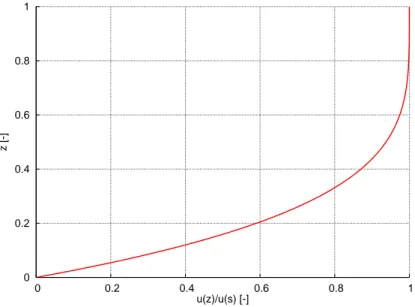
Fig. 1. 2-D flowline steady-state manufactured solution (coefficientλ=4): horizontal component of velocity scaled to the surface velocity
as a function of dimensionless thickness. Horizontal velocity increases with the fourth power of ice thickness. Most shearing ice concentrated near the glacier base which is similar to lamellar flow.
whereϑis an arbitrary function of one variable.
The formula (36) shows that the functions satisfying the kinematic boundary conditions (13–14) and the conservation of mass Eq. (9), derived under assumption (21), depend on the form of the functionϑand ice surface and bed curves.
To generate a solution similar to the benchmark experi-ment B in (Pattyn et al., 2008) and to keep the mathematics simple, choose functionϑas follows:
ϑ (x)=cx1−(1−x)λ+cb, (37)
whereλ,cx, andcbare constants. The first term on the
right-hand side of (37) may be considered as component of veloc-ity associated with internal deformation, andcbas the basal
sliding velocity coefficient.
Then the velocity field satisfying the 2-D versions of the kinematic boundary conditions (13–14) and the conservation of mass Eq. (9) is:
u(x,z,t )= cx
s−b
"
1−
s−z s−b
λ# + cb
s−b− 1 s−b
Z
∂s ∂t− ˙a
dx,(38)
w(x,z,t )=u(x,z,t )
db
dx s−z s−b+
∂s ∂x
z−b s−b
+
∂s
∂t− ˙a
z−b
s−b, (39)
For a zero-accumulation(a˙=0)steady-state(∂s∂t =0)flow with frozen bed(cb=0), the horizontal velocity scaled to
the surface velocity can be written as a function of ice scaled depthd=ss−−zb:
u(x,z,t )=u(x,s,t ) "
1−
s−z s−b
λ#
=u(x,s,t )1−dλ. (40)
This expression shows that the horizontal velocity from in-ternal deformation increases with powerλof ice depth. For λ=4 this is consistent with lamellar flow (der Veen, 1999) as shown in Fig. 1.
As can be seen from (38) for a zero-accumulation(a˙=0) steady-state(∂s∂t =0)flow, ifλ >0, then
cb=u(x,b)(s−b)=u(x,b)hand
cx=[u(x,s)−u(x,b)](s−b)=[u(x,s)−u(x,b)]h.
These expressions show thatcbcan be interpreted as the
ice-flux due to sliding flow andcxcan be interpreted as the
ice-flux due to deformation flow.
In addition to velocities, the ice pressure function should also be constructed.
The manufactured solution for the ice pressure can be cho-sen, for example, as in Pattyn’s higher-order model (Pattyn, 2003):
˜
p=σx′˜x˜− ˜ρg(˜ s˜− ˜z)=2µ˜∂u˜
∂x˜− ˜ρg(˜ s˜− ˜z),
or in nondimensional form:
p(x,z,t )=2µ∂u
∂x−(s−z). (41)
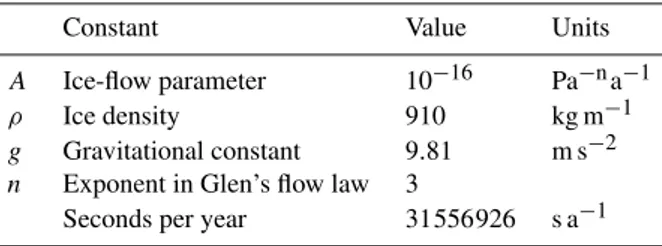
Table 1. Constants for the benchmark experiments.
Constant Value Units
A Ice-flow parameter 10−16 Pa−na−1
ρ Ice density 910 kg m−1
g Gravitational constant 9.81 m s−2 n Exponent in Glen’s flow law 3
Seconds per year 31556926 s a−1
functions into exact solutions of these equations, we substi-tute them into the equations and calculate the right-hand side functions that match these solutions. This can be done when a specific surfaces(x,t )and bedb(x)are chosen.
Equations (38–39) also satisfy prognostic equation de-scribing the change of local ice thicknessh(x,t )=s(x,t )− b(x)in space:
∂h ∂t = ˙a−
∂ ∂x
Z s
b
udz. (42)
Equations (38–39) and (41) are solutions of flow with a gen-eral surfaces(x,t) and bedb(x). Below are specific solu-tions for a particular case of an ice surface and a sinusoidal bed, similar to the benchmark experiment B in (Pattyn et al., 2008).
3.2 A manufactured solution for a time-dependent flow with a sinusoidal bed
To generate a particular solution, assume a flow with zero accumulation/ablation rate, a˙=0, a sinusoidal bed defined as in (Pattyn et al., 2008), and an ice surface that changes from a linear sloping surface to the one that is draped over the topography of the bed:
s(x,t )=s0(x)+η(x)γ (t ), s0(x)= −x·tan(α), (43)
b(x)=s0(x)−1+η(x), (44)
where η(x)=1
2sin(2π x), γ (t )=1−e
−ctt, c
t is a constant. (45)
Constantct shows how fast the ice surface changes
(rela-tive to the value of the ice bed) at the beginning of the test: ct=η(x)1 ∂s∂t|t=0.
For a flow down an infinite plane with a mean inclination tan(α), periodic boundary conditions for a functionf are de-fined as follows:f (0,z+tan(α))=f (1,z)and the analytical solutions (38), (39), (41) satisfy these conditions for geome-try (43–44).
Appendix A contains the formulas and supplement to this manuscript contains a simple fortran 77 code that can be used to calculate the exact solutions and compensatory stress terms for the momentum equation in the 2-D flowline model. The code dumps the generated solutions to specified files. All input data are specified in file parameter2d.h in the supplement.
Values of flow parameters and constants are chosen from (Pattyn et al., 2008) and are given in Table (1), the start-ing linear slope of the ice surfaceα=0.5◦. The length scale of the domain is chosen 80 km, which results in aspect ratio δ=1/80.
Constants of the test are chosen as follows: coefficient in (45) ct=10−6 and coefficients in (38) cx=10−6,cb=
10−6, andλ=4. This experiment can be considered as an ice-stream flow over a bumpy bed. The values of constants cx,cb, andct chosen to generate a reasonable dimensional
cx=cb=uh=
˜ u
U ˜ h
Z= ˜ u
(2ρ˜gZ)˜ nAL ˜ h
Z=
45000 ma−1 2×910 kg m−19.81 ms−21000 m3
10−16Pa−3a−180000 m
1000 m 1000 m≈10
−6.
The choice of parameterctwas dictated by the typical scale value of the time parameter:
ct≈T=
Z
W =
L
U =
L (2ρ˜gZ)˜ nAL=
1 (2ρ˜gZ)˜ nA=
1
2×910 kg m−19.81 m s−21000 m3
10−16Pa−3a−1≈1.7×10
−6a
Velocity is shown in km/yr and pressure in MPa.
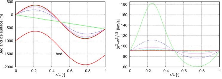
Figure (2) shows the bed (44) and the time-evolution of the ice surface (43) (left graph) and the time-evolution of the norm of the surface velocity (right graph) over 14-year period. The ice surface changes from a linear sloping sur-face to the sursur-face draped over the topography of the bed. Ice thickness is spatially uniform when the steady-state so-lution is reached. The surface velocity at the beginning is anti-correlated with the ice thickness – it is larger over the bump than over the trough. At the steady-state, the surface velocity is spatially uniform and does not depend on the bed topography.
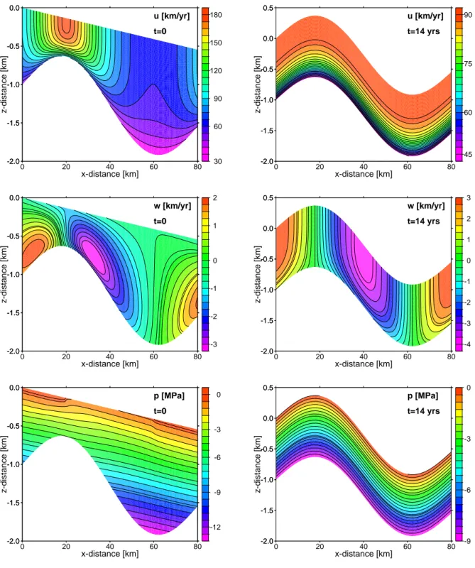
Figure (3) shows the horizontal velocity, vertical velocity, and pressure at the beginning (left graphs) and at the time when the steady-state solution is reached (right graphs).
Figure (4) shows the compensatory horizontal and verti-cal stress terms in the conservation of momentum equation at the beginning (left) and at the time when the steady-state solution is reached (right). At the beginning both stress terms have largest values over the bump. At the steady-state solu-tion, the stress terms are zeroes almost everywhere except a small surface layer over the bump.
3.3 A steady-state manufactured solution for a flow with a linear sloping surface and a sinusoidal bed To generate a steady-state solution, assume that in (43) the functionγ (t )=0, that is, a linear sloping surface and a sinu-soidal bed are defined similar to the ones of the benchmark experiment B in (Pattyn et al., 2008):
s(x)= −x·tan(α), (46)
b(x)=s(x)−1+1
2sin(2π x). (47)
If we substitute the above functions for bed and surface into (38–39), then the corresponding steady-state flow’s veloci-ties are as follows:
u(x,z)= cx
1−12sin(2π x)
1−
−z−xtan(α) 1−12sin(2π x)
!λ
(48)
+ cb
1−12sin(2π x),
w(x,z)=u(x,z) db
dx s−z s−b+
ds dx
z−b s−b
. (49)
Choice of coefficientcb=0 generates frozen bed flow with
zero basal velocities, whilecb6=0 generates flow with a
slid-ing bed.
As can be seen from (48–49), ifλ >0 then atz=b, u(x,b)=0, w(x,b)=0;
atz=s,u(x,s)= cx s−b =
cx
h, w(x,s)=
ds dx
h .
The last expression shows the conservation of mass flux, q=hu=cx=constant. This anti-correlated relationship
be-tween surface horizontal velocity and ice thickness is consis-tent with the simulation of the smallest length scaleL=5km Experiment B in (Pattyn et al., 2008), by all full-Stokes mod-els.
Figure (5) shows the horizontal and vertical velocity, ice pressure, and the norm of the surface velocity correspond-ing to the flow with a linear slopcorrespond-ing surface with a slope α=0.5◦and afrozensinusoidal bed (cb=0). The constants
in (48) are chosen ascx=10−6andλ=4.0 and the aspect
ratioδ=1/80.
4 Analytical manufactured solutions of the 3-D isothermal full-Stokes ice-flow model
Assume as in the 2-D case that in the interior of the domain, s(x,y,t ) > b(x,y), the vertical velocitywis:
w(x,y,z,t)=u(x,y,z,t ) ∂b
∂x s−z s−b+
∂s ∂x
z−b s−b
(50)
+v(x,y,z) ∂b
∂y s−z s−b+
∂s ∂y
z−b s−b
+ ∂s
∂t − ˙a z−b
s−b,
then the kinematic boundary conditions (13–14) are satisfied. From (50), it follows that
∂w ∂z =
∂u ∂z
∂b
∂x s−z s−b+
∂s ∂x
z−b s−b
(51)
+u
∂s
∂x−
∂b ∂x
s−b + ∂v ∂z
∂b ∂y
s−z s−b+
∂s ∂y
z−b s−b
+v
∂s ∂y−
∂b ∂y
s−b + 1 s−b
∂s ∂t − ˙a
-2000 -1500 -1000 -500 0 500
0 0.2 0.4 0.6 0.8 1
Bed and ice surface [m]
x/L [-] bed
60 80 100 120 140 160 180
0 0.2 0.4 0.6 0.8 1
(u
2 +w 2 )
1/2
[km/a]
x/L [-]
Fig. 2.2-D flowline time dependent experiment – ice stream flow over bumpy bed; the steady bed and transformation over time of the ice
surface (left) and transformation over time of the norm of the surface velocity (right). Ice surface and the norm of the surface velocity are shown every 1.5 years over the 14-year period, green curves are the initial values and red curves are the final values.
If we substitute (51) into the incompressibility Eq. (9), we obtain the following equation containing only variablesu,v and their derivatives:
∂u
∂x+ ∂u
∂z ∂b
∂x s−z
s−b+ ∂s
∂x z−b
s−b
+u
∂s
∂x−
∂b ∂x
s−b (52)
+∂v ∂y+
∂v ∂z
∂b ∂y
s−z s−b+
∂s ∂y
z−b s−b
+v
∂s ∂y−
∂b ∂y
s−b
+ 1
s−b ∂s
∂t− ˙a
=0.
Equation (52) is a first-order quasi-linear partial differen-tial equation with three independent variables (x,y, andz) and two dependent variables (uandv) of type:
F
x,y,z,u(x,y,z,t ),v(x,y,z,t ),∂u ∂x,
∂u ∂z,
∂v ∂y,
∂v ∂z
=0. (53)
Similar to the 2-D flowline manufactured solutions, we choose velocityu(x,y,z,t )as the following function:
u(x,y,z,t)=cx(s−b)γ1
" 1−
s −z s−b
λ1# +cbx
1
s−b, (54) or
u(x,y,z,t)=cxhγ1 1−dλ1
+cbx
1 h,
where γ1, λ1, cx, cbx are constants, d(x,y,z,t )=ss−−zb is
scaled ice depth, andh(x,y,t )=s−bis ice thickness. Then the derivatives of functionu(x,y,z,t )are
∂u ∂x=cxγ1h
γ1−1∂h
∂x 1−d
λ1
−cxλ1hγ1dλ1−1 ∂d ∂x−
cbx h2
∂h ∂x, (55) ∂u
∂z=cxλ1h
-2.0 -1.5 -1.0 -0.5 0.0
-2.0 -1.5 -1.0 -0.5 0.0
z-distance [km]
0 20 40 60 80
x-distance [km]
30 60 90 120 150 180 u [km/yr]
t=0
-2.0 -1.5 -1.0 -0.5 0.0 0.5
-2.0 -1.5 -1.0 -0.5 0.0 0.5
z-distance [km]
0 20 40 60 80
x-distance [km]
45 60 75 90 u [km/yr]
t=14 yrs
-2.0 -1.5 -1.0 -0.5 0.0
-2.0 -1.5 -1.0 -0.5 0.0
z-distance [km]
0 20 40 60 80
x-distance [km]
-3 -2 -1 0 1 2 w [km/yr]
t=0
-2.0 -1.5 -1.0 -0.5 0.0 0.5
-2.0 -1.5 -1.0 -0.5 0.0 0.5
z-distance [km]
0 20 40 60 80
x-distance [km]
-4 -3 -2 -1 0 1 2 3 w [km/yr]
t=14 yrs
-2.0 -1.5 -1.0 -0.5 0.0
-2.0 -1.5 -1.0 -0.5 0.0
z-distance [km]
0 20 40 60 80
x-distance [km]
-12 -9 -6 -3 0 p [MPa]
t=0
-2.0 -1.5 -1.0 -0.5 0.0 0.5
-2.0 -1.5 -1.0 -0.5 0.0 0.5
z-distance [km]
0 20 40 60 80
x-distance [km]
-9 -6 -3 0 p [MPa]
t=14 yrs
Fig. 3.2-D flowline time dependent experiment – ice stream flow over bumpy bed. The graphs show the horizontal velocityu, the vertical
-2.0 -1.5 -1.0 -0.5 0.0
-2.0 -1.5 -1.0 -0.5 0.0
z-distance [km]
0 20 40 60 80
x-distance [km]
-6.0 -4.5 -3.0 -1.5 0.0
Σx [kJ]
t=0
-2.0 -1.5 -1.0 -0.5 0.0 0.5
-2.0 -1.5 -1.0 -0.5 0.0 0.5
z-distance [km]
0 20 40 60 80
x-distance [km]
-30 -20 -10 0
Σx [kJ]
t=14 yrs
-2.0 -1.5 -1.0 -0.5 0.0
-2.0 -1.5 -1.0 -0.5 0.0
z-distance [km]
0 20 40 60 80
x-distance [km]
-2 -1 0 1 2
Σz [kJ]
t=0
-2.0 -1.5 -1.0 -0.5 0.0 0.5
-2.0 -1.5 -1.0 -0.5 0.0 0.5
z-distance [km]
0 20 40 60 80
x-distance [km]
-10 -5 0 5 10
Σz [kJ]
t=14 yrs
Fig. 4.2-D flowline time dependent experiment – ice stream flow over bumpy bed. The graphs show the compensatory horizontal6xand
-2.0 -1.5 -1.0 -0.5 0.0
-2.0 -1.5 -1.0 -0.5 0.0
z-distance [km]
0 20 40 60 80
x-distance [km]
0 15 30 45 60 75 90 u [km/yr]
steady-state experiment
-2.0 -1.5 -1.0 -0.5 0.0
-2.0 -1.5 -1.0 -0.5 0.0
z-distance [km]
0 20 40 60 80
x-distance [km]
-1.2 -0.8 -0.4 0.0 0.4 0.8 w [km/yr]
steady-state experiment
-2.0 -1.5 -1.0 -0.5 0.0
-2.0 -1.5 -1.0 -0.5 0.0
z-distance [km]
0 20 40 60 80
x-distance [km]
-12 -9 -6 -3 0 p [MPa]
steady-state experiment
30 40 50 60 70 80 90
0 0.2 0.4 0.6 0.8 1
(u
2 +w 2 )
1/2
[km/a]
x/L [-]
Fig. 5. 2-D flowline steady-state experiment - version of experiment B from (Pattyn et al., 2008) (flow with a linear sloping surface and
a sinusoidalfrozenbed); the graphs show horizontaluand verticalwvelocity in [km/yr], the ice pressure in [MPa] and the norm of the
surface velocityu2+w2 1/2
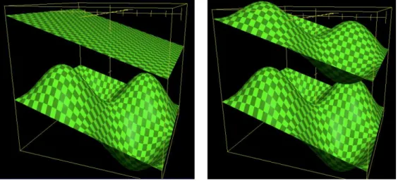
Fig. 6. 3-D time dependent experiment – ice flow over a bumpy bed. The graphs show the bed and ice surface at the beginning (left) and at the steady state (right). All distances are scaled. Ice flow is from left to right. The ice surface changes from a linear sloping surface to the surface draped over the topography of the bed. Ice thickness is spatially uniform when the steady-state solution is reached.
0 20 40 60 80
0 20 40 60 80
y-distance [km]
0 20 40 60 80
x-distance [km]
25 35 45 55 65 surface u [km/yr], t=0
0 20 40 60 80
0 20 40 60 80
y-distance [km]
0 20 40 60 80
x-distance [km]
0 30 60 90 surface v [km/yr], t=0
Fig. 7. 3-D time-dependent experiment. The left and right graphs show the ice surfacex- andy- horizontal velocity respectively at the
beginning. At the time when the steady-state solution is reached, both velocities at the surface are uniform and have values of 46 km/yr.
Substituting (54) and (55) into (52) and using relations ∂b∂yss−−zb+∂y∂szs−−bb=h∂d∂x generates a first-order quasi-linear partial differential equation with four independent variables (x,y,z, andt) and only one dependent variable (v):
∂v ∂y+
∂v ∂z
b′ys−z
s−b+s
′
y
z−b s−b
+vs
′
y−b′y
0 20 40 60 80
0 20 40 60 80
y-distance [km]
0 20 40 60 80
x-distance [km]
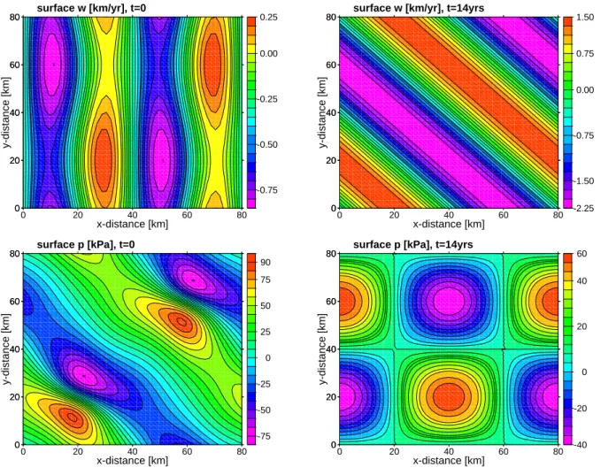
-0.75 -0.50 -0.25 0.00 0.25 surface w [km/yr], t=0
0 20 40 60 80
0 20 40 60 80
y-distance [km]
0 20 40 60 80
x-distance [km]
-2.25 -1.50 -0.75 0.00 0.75 1.50 surface w [km/yr], t=14yrs
0 20 40 60 80
0 20 40 60 80
y-distance [km]
0 20 40 60 80
x-distance [km]
-75 -50 -25 0 25 50 75 90 surface p [kPa], t=0
0 20 40 60 80
0 20 40 60 80
y-distance [km]
0 20 40 60 80
x-distance [km]
-40 -20 0 20 40 60 surface p [kPa], t=14yrs
Fig. 8.3-D time dependent experiment; the graphs show the ice surface vertical velocityw(in km/yr) and the ice surface pressurep(in kPa)
at the beginning (left) and at the time when the steady-state solution is reached (right).
The characteristic system of Eq. (56) is as follows: d y
1 =
d z
b′
yss−−bz+sy′zs−−bb
(57)
= − d v
vs ′
y−b′y
s−b +cx(γ1+1)(sx′−b′x)(s−b)γ1−1
1−ss−−zbλ1
+s−1b ∂s∂t − ˙a .
Two independent particular solutions of this system can be found by solving the equations: dy
1 =
dz
b′
yss−−zb+sy′zs−−bb
, (58)
dy 1 = −
dv
vs ′
y−b′y
s−b +cx(γ1+1)(sx′−bx′)(s−b)γ1−1
1−ss−−bzλ1
+s−1b ∂s∂t− ˙a
-2.0 -1.5 -1.0 -0.5 0.0
-2.0 -1.5 -1.0 -0.5 0.0
z-distance [km]
0 20 40 60 80
x-distance [km]
0 30 60 90 (u2+v2+w2)1/2 [km/yr]
at y=L/4
t=0
-2.0 -1.5 -1.0 -0.5 0.0 0.5
-2.0 -1.5 -1.0 -0.5 0.0 0.5
z-distance [km]
0 20 40 60 80
x-distance [km]
0.6 15.0 30.0 45.0 60.0 (u2+v2+w2)1/2 [km/yr]
at y=L/4
t=14 yrs
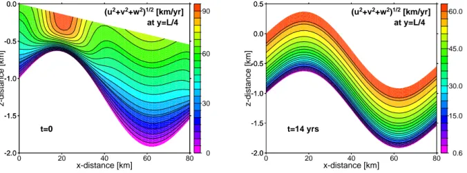
Fig. 9. 3-D time-dependent experiment. The graphs show the the norm of the velocityu2+v2+w21/2along they=1/4 slide at the
beginning (left) and at the time when the steady-state is reached (right). At the beginning, velocity has two local maximums, over the bump and over the bed where the bed changes the most. At the steady-state position, velocity is spatially uniform and proportional to the ice thickness.
-1000 -800 -600 -400 -200 0 200 400
0 0.2 0.4 0.6 0.8 1
Ice surface [m]
x/L [-]
60 65 70 75 80 85 90 95
0 0.2 0.4 0.6 0.8 1
(u
2 +v 2 +w 2 )
1/2
[km/yr]
x/L [-]
Fig. 10. 3-D time dependent experiment; the ice surface elevation (left) and the norm of the surface velocityu2+v2+w21/2(right)
change alongy=1/4 slide. Ice surface and the norm of the surface velocity are shown every 1.5 years over the 14-year period, green curves are the initial values and red curves are the final values. At the beginning, velocity has two local maximums, over the bump and over the bed where the bed changes the most. At the steady-state position, the norm of the surface velocity is spatially uniform.
This is a first-order ordinary differential equation. The solution of the homogeneous equation is v=a(y)
s−b. (62)
wherea(y)is an unknown function.
Substituting Eq. (62) into Eq. (61), we obtain an equation fora:
a′(y)= −cx(γ1+1)(sx′−b′x)(s−b)γ1
" 1−
s−z s−b
λ1# −
∂s ∂t − ˙a
,
which has a solution: a(y)= −
Z (
cx(γ1+1)(sx′−b
′
x)(s−b) γ1
" 1−
s−z s−b
λ1# +
∂s ∂t − ˙a
)
dy+c2. (63)
Substituting (63) into Eq. (62), we obtain
v= −R
cx(γ1+1)(sx′−b′x)(s−b)γ1
1−ss−−zb
λ1
+ ∂s∂t− ˙a
dy+c2
s−b or
c2=v(s−b)+
Z (
cx(γ1+1)(sx′−b′x)(s−b)γ1
" 1−
s−z s−b
λ1# +
∂s ∂t− ˙a
)
dy (64)
Then, the general solution of Eq. (56) can be written as
θ v(s−b)+ Z (
cx(γ1+1)(sx′−b
′
x)(s−b) γ1
" 1−
s−z s−b
λ1# +
∂s ∂t− ˙a
)
dy,z−b s−b !
=0, (65)
whereθis an arbitrary function of two variables. With Eq. (65) solved forv, the general solution can be written in the form
v(x,y,z,t )= 1 s−bϑ
z −b s−b
− 1
s−b Z (
cx(γ1+1)(sx′−b
′
x)(s−b)γ1
" 1−
s −z s−b
λ1# +
∂s ∂t− ˙a
)
dy, (66)
whereϑis an arbitrary function of one variable.
If we assume again that functionϑin (66) is of the form
ϑ (x)=cy1−(1−x)λ2+cby, (67)
whereλ2,cy, andcbyare constants, then functions (54), (50), and (66) satisfying the mass balance equation and the kinematic
boundary conditions are as follows:
u(x,y,z,t )=cx(s−b)γ1
" 1−
s −z s−b
λ1# +cbx
1
s−b, (68)
v(x,y,z,t )= cy s−b
" 1−
s−z s−b
λ2# +cby
1 s−b−
1 s−b
Z (
cx(γ1+1)(sx′−b′x)(s−b)γ1 "
1−
s−z s−b
λ1# +
∂s ∂t− ˙a
)
dy, (69)
w(x,y,z,t )=u(x,y,z) ∂b
∂x s−z s−b+
∂s ∂x
z−b s−b
+v(x,y,z) ∂b
∂y s−z s−b+
∂s ∂y
z−b s−b
+
∂s ∂t − ˙a
z −b
The manufactured solution for the ice pressure can be chosen again as in Pattyn’s higher-order model (Pattyn, 2003):
˜
p=σx′˜x˜+σy′˜y˜− ˜ρg(˜ s˜− ˜z)=2µ˜∂u˜ ∂x˜+2µ˜
∂v˜
∂y˜− ˜ρg(˜ s˜− ˜z),
or in nondimensional form: p=2µ∂u
∂x+2µ ∂v
∂y−(s−z), (71)
where non-dimensional ice viscosity
µ= "
1 4
∂u ∂y+
∂v ∂x
2 +1
4
1 δ
∂u ∂z+δ
∂w ∂x
2 +1
4
1 δ
∂v ∂z+δ
∂w ∂y
2 −∂u
∂x ∂v ∂y−
∂u ∂x
∂w ∂z −
∂v ∂y
∂w ∂z
1−2nn
. (72)
The constructed velocities satisfy the surface and bed kinematic boundary conditions (13–14) and the mass conservation Eq. (9). However, the constructed velocities and pressure do not necessarily satisfy the conservation of momentum equations and the basal and surface boundary conditions. To make the constructed functions into exact solutions of these equations, we substitute them into those equations and calculate the right-hand side functions which accommodate the solutions. This can be done when specific surfaces(x,y,t )and bedb(x,y)are chosen.
The constructed solutions do not satisfy ice-sheet evolu-tion equaevolu-tion describing the change of local ice thickness h(x,y,t )=s(x,y,t )−b(x,y)in space:
∂h ∂t = ˙a−
∂ ∂x
Z s
b
udz− ∂ ∂y
Z s
b
vdz. (73)
To make the constructed functions into exact solutions of Eq. (73), the equation can be modified by adding to the right-hand side of the equation a compensatory term.
4.1 A time-dependent analytical solution for a flow with a sinusoidal bed
To generate a particular solution, assume a flow with a sinu-soidal bed defined similar to the bed in the benchmark experi-ment A in (Pattyn et al., 2008) and an ice surface that changes
from a linear sloping surface to the one that is draped over the bed:
s(x,y,t )=s0(x)+η(x,y)γ (t ), s0(x)= −x·tan(α), (74)
b(x,y)=s0(x)+η(x,y)−1, (75)
where η(x,y)=1
2sin(2π x)sin(2πy),γ (t )=1−e
−ctt, c
t is a constant.
To calculate integral in (69), substitute functions (74–75) for bed and surface into the integral in (69). Since it is diffi-cult to calculate the integral analytically for general constants γ1andλ1, particular values, for example,γ1=1 andλ1=1,
4.1.1 Parametersγ1=1,λ1=1
I=
Z
2cx(z−b)(sx′−b′x)+
∂s ∂t − ˙a
dy
= Z
[z−s0(x)+1−η(x,y)]2cxη′x(γ (t )−1)+γ
′(t )η
− ˙a dy
=2π cx(γ (t )−1)cos(2π x)
Z
z−s0(x)+1−
1
2sin(2π x)sin(2πy)
sin(2πy)dy
+γ
′(t )
2 sin(2π x) Z
sin(2πy)dy− Z
˙ ady
=2π cx(γ (t )−1)cos(2π x)
−z−s0(x)+1
2π −
1
4sin(2π x) Z
[1−cos(4πy)]dy
−γ
′(t )
4π sin(2π x)cos(2πy)− ˙ay
=cx(1−γ (t ))cos(2π x)cos(2πy)(z−s0(x)+1)−
γ′(t )
4π sin(2π x)cos(2πy) (76)
+hπ
4cx(1−γ (t ))sin(4π x)− ˙a i
y−cx
16(1−γ (t ))sin(4π x)sin(4πy).
If we substitute the calculated integral and functions (74– 75) for bed and surface into (68–70), we obtain the following formulas for velocities:
u(x,y,z,t )=cx(z−b)+cbx
1
s−b, (77)
v(x,y,z,t )= cy s−b
"
1−
s−z s−b
λ2#
− I
s−b+cby 1
s−b, (78)
w(x,y,z,t )=u(x,y,z,t ) ∂b
∂x s−z s−b+
∂s ∂x
z−b s−b
(79)
+v(x,y,z,t ) ∂b
∂y s−z s−b+
∂s ∂y
z−b s−b
+
∂s ∂t − ˙a
z −b s−b.
For a flow down an infinite plane with a mean incli-nation tan(α), periodic boundary conditions for a function f are defined as follows: f (0,y,z+tan(α))=f (1,y,z), f (x,0,z+tan(α))=f (x,1,z).
The constructed solutions (77–79), (71) satisfy periodic boundary conditions only in the horizontalx- direction and do not satisfy periodic boundary conditions in the horizon-tal y- direction for all values of the input parameters. To satisfy periodic boundary conditions in all lateral directions, the accumulation-ablation rate may be chosen as follows:
˙
a= ˙a(x,t )=(π/4)cx(1−γ (t ))sin(4π x).
Appendix 4.1.1 contains the formulas that can be used to calculate the compensatory stress terms for the momentum equation. For the 3-D ice-stream flow over a bumpy bed ex-periment, the parameters of the flow are chosen as follows:
the horizontal domain is chosen 80 km×80km which results in aspect ratioδ=1/80, the starting linear slope of the ice surfaceα=0.5◦, sliding bed parameterscbx=cby=10−8,
and the remaining constants in (77) and (78)cx=cy=10−6,
λ2=4, andct=10−6. As in 2-D case, all graphs are given
for the dimensional values of variables which are calculated from non-dimensional values using formulas (6).
Figure (6) shows the bed (75) and the ice surface (74) at the time zero and at the time when the steady-state solution is reached. Ice flow is from left to right. The ice surface changes from a linear sloping surface to the surface draped over the topography of the bed. Ice thickness is spatially uni-form when the steady-state solution is reached.
Figure (7) shows the horizontal and vertical velocity at the beginning. At the steady-state, the horizontal velocity field is smoothed out, bothx- andy- horizontal velocities are almost spatially uniform (≈46 km/yr).
Figure (8) shows the vertical velocity and pressure at the beginning and at the time when the steady-state solution is reached.
Figure (9) shows the norm of the velocity along they=
4.2 A steady-state analytical solution for a flow with a linear sloping surface and a sinusoidal bed
To generate a steady-state solution, assume that in (74) the functionγ (t )=0, that is, a linear sloping surface and a slop-ing sinusoidal bed are defined as in the benchmark experi-ment A in (Pattyn et al., 2008).
s(x,y)= −x·tan(α), (80)
b(x,y)=s(x,y)−1+1
2sin(2π x)sin(2πy). (81) The coefficients are α=0.5◦, λ2=2.25, cx=cy=
1, cbx=cby =0, δ=1/80, and accumulation rate a˙= πsin(4π x)
4 .
All functions, the surface horizontalx- andy- velocities, the verticalz- velocities as well as the surface ice pressure, for this steady-state experiment are very similar to the cor-responding graphs in Figs. (7) and (8) of the time-dependent experiment at the beginning time.
5 Conclusions
The detailed constructions of manufactured exact solutions to 3-D and 2-D flowline time-dependent and steady-state isothermal full-Stokes ice sheet problems are presented. The solutions are valid for non-linear Glen-type flow. The con-struction of exact solutions done by using manufactured so-lution technique (Bueler et al., 2007) while the suggested experiments follow directly from ice sheet intercompari-son (Pattyn et al., 2008).
The steady-state solutions, constructed in this paper, are variations of the benchmark experiments A and B in (Pat-tyn et al., 2008). However, by substituting different ice sur-face and bed geometry formulas into the derived formulas, analytical solutions for different geometries can also be con-structed.
Although artificially constructed, the solutions may be useful for testing numerical methods. They offer several
ben-efits to potential ice sheet modelers. By changing a param-eter value, the analytical solutions will allow the modelers to investigate their algorithms for a different range of as-pect ratios as well as for different, frozen or sliding, basal boundaries. The lateral boundary conditions can be speci-fied as periodic boundary conditions or as essential Dirichlet conditions. Specifying Dirichlet conditions, when the exact solutions are specified as inflow and outflow boundary con-ditions, allows the modelers to check the model accuracy in the inside of the problem domain.
Appendix A
Calculation of compensatory stress functions in the 2-D flowline full-Stokes diagnostic equations
A1 Compensatory terms in diagnostic equations and in the boundary conditions
The constructed velocities (38–39) satisfy the 2-D versions of the surface and bed kinematic boundary conditions (13– 14) and the mass conservation Eq. (9) but do not necessarily satisfy the conservation of momentum Eqs. (10–12) and its basal and surface boundary conditions (15–17) and (18–20). Following (Bueler et al., 2007), we introduce compensatory stresses6x and6zin the conservation of momentum
equa-tions to make the chosen velocity and pressure funcequa-tions into exact solutions of the equations.
δ∂ 2µ
∂u ∂x+p
∂x +
∂µ1δ∂u∂z+δ∂w∂x
∂z =6x, (A1)
δ
∂µδ∂w∂x +1δ∂u∂z
∂x +
∂2µ∂w∂z +p
∂z −1=6z, (A2)
To make the chosen velocities satisfy the boundary condi-tions, we introduce compensatory termsυx,υz,τb, andτzin
At the upper surfaces(x,t ), the boundary conditions are as follows: 1
q
1+δ2 ds dx
2
−δds dx
2µ∂u
∂x+p +µ 1 δ ∂u
∂z+δ ∂w
∂x
=υx, (A3)
1 q
1+δ2 ds dx
2
−δds dx µ δ∂w ∂x+ 1 δ ∂u ∂z + 2µ∂w
∂z +p
=υz. (A4)
At the lower surfaceb(x), they are as follows: 1
q
1+δ2 db dx 2 δdb dx 2µ∂u
∂x+p −µ 1 δ ∂u ∂z+δ
∂w ∂x
=τx, (A5)
1 q
1+δ2 db dx 2 δdb dx µ δ∂w ∂x+ 1 δ ∂u ∂z − 2µ∂w
∂z+p
+1=τz. (A6)
A2 Calculation of derivatives
Calculation of the compensatory stress terms requires calculation of derivatives of the exact solutions (38), (39), and (41). To simplify calculation of the derivatives, we re-write these functions as follows:
u(x,z,t )= 1 h
cx 1−dλ+cb−
Z ∂s ∂t − ˙a
dx
, (A7)
w(x,z,t )=uh∂d ∂x+
∂s ∂t − ˙a
(1−d), (A8)
whereh=h(x,t )is ice thickness andd=d(x,z,t )=ss−−zbis scaled ice depth. Then, the first derivatives of functions (A7–A8) are
∂u ∂z =
cxλ
h2d λ−1,
∂u
∂x = − 1 h
∂h
∂xu+cxλd
λ−1∂d
∂x+ ∂s
∂t − ˙a
= −1 h
∂h
∂xu+h
2∂u
∂z ∂d
∂x+ ∂s
∂t − ˙a
,
∂w ∂z = −
∂u
∂x, (A9)
∂w ∂x =
∂u ∂xh
∂d ∂x+u
∂h ∂x
∂d ∂x+uh
∂2d ∂x2+
∂2s ∂x∂t−
∂a˙ ∂x
!
(1−d)− ∂s
∂t− ˙a
∂d
∂x,
and the second derivatives are ∂2u
∂z2 = −
cxλ(λ−1)
h3 d
λ−2, (A10)
∂2u ∂x2= −
1 h "
∂2h ∂x2u+2
∂h ∂x
∂u ∂x−h
3∂2u
∂z2
∂d ∂x
2 +h2∂u
∂z ∂2d ∂x2+
∂2s ∂x∂t−
∂a˙ ∂x #
,
∂2u ∂x∂z= −
2cxλ
h3 d λ−1∂h
∂x+
cxλ(λ−1)
h2 d
λ−2∂d
∂x= − 1 h 2 ∂u ∂x ∂u ∂z+ ∂d ∂x
∂2u ∂z2
! ,
∂2w ∂x2 =
∂2u ∂x2h
∂d ∂x+2
∂u ∂x
∂h ∂x
∂d ∂x+2
∂u ∂xh
∂2d ∂x2+u
∂2h ∂x2
∂d ∂x+2u
∂h ∂x
∂2d ∂x2+uh
∂3d ∂x3
+ ∂
3s
∂x2∂t−
∂2a˙ ∂x2
!
(1−d)−2 ∂
2s
∂x∂t− ∂a˙ ∂x
! ∂d ∂x−
∂s ∂t− ˙a
∂2d
∂x2,
∂2w
∂x∂z= − ∂2u
∂x2,
∂2w ∂z2 = −
where, for a surface (43) and a sinusoidal bed (44), ∂h
∂x=η
′(x)(γ (t )−
1), ∂s ∂x=s
′
0(x)+η′(x)γ (t ), (A11)
∂s
∂t =η(x)γ
′(t ),Z ∂s
∂tdx=γ
′(t )Z η(x)dx,
∂2s ∂x∂t=η
′(x)γ′(t ), ∂3s
∂x2∂t=η
′′(x)γ′(t ),
∂2h ∂x2=η
′′(x)(γ (t )
−1),∂
3h
∂x3=η
′′′(x)(γ (t )
−1), ∂2s
∂x2=η
′′(x)γ (t ), ∂3s
∂x3=η
′′′(x)γ (t ),
∂d ∂x=
1 h
∂s ∂x−
∂h ∂xd
,∂d
∂z= − 1 h,
∂2d ∂x2=
1 h
" ∂2s ∂x2−2
∂h ∂x
∂d ∂x−
∂2h ∂x2d
# ,
∂3d ∂x3=
1 h
" ∂3s ∂x3−3
∂2h ∂x2
∂d ∂x−3
∂h ∂x
∂2d ∂x2−d
∂3h ∂x3
#
If we name the expression ν=1
2
1 δ
∂u ∂z+δ
∂w ∂x
2 −∂u
∂x ∂w
∂z, (A12)
thenµ=ν1−2nn.
For further calculations we need the following derivatives: ∂µ
∂x = 1−n
2n µ ν "
1 2
1 δ
∂u ∂z+δ
∂w ∂x
1 δ
∂2u ∂x∂z+δ
∂2w ∂x2
! −∂
2u
∂x2
∂w ∂z−
∂u ∂x
∂2w ∂x∂z
#
, (A13)
∂µ ∂z =
1−n 2n
µ ν "
1 2
1 δ
∂u ∂z+δ
∂w ∂x
1 δ
∂2u
∂z2+δ
∂2w ∂x∂z
! − ∂
2u
∂x∂z ∂w
∂z − ∂u ∂x
∂2w
∂z2
#
, (A14)
Substituting (A9–A10) and (A13–A14) into (A1–A2), (A3–A4), and (A5–A6) generate formulas for compensatory terms 6x,6z,υx,υz,τx, andτz.
If constantλin (37) is chosen so thatλ >2, then the calculation of the second derivatives is well defined.
Appendix B
Calculation of compensatory stress functions in 3-D full-Stokes diagnostic equations B1 Compensatory terms in diagnostic equations and in the boundary conditions
δ
∂µδ∂w∂x+1δ∂u∂z
∂x +δ
∂µδ∂w∂y +1δ∂v∂z
∂y +
∂2µ∂w∂z+p
∂z −1=6z. (B3)
To make the chosen velocities satisfy the boundary conditions, we introduce compensatory termsυx,υy,υz,τx,τy, andτzin
the boundary conditions.
At the upper surfaces(x,y,t ), the boundary conditions are as follows: 1
rs
−δ∂s
∂x
2µ∂u ∂x+p
−δ∂s
∂yµ ∂u
∂y+ ∂v ∂x
+µ
1 δ
∂u ∂z+δ
∂w ∂x
=υx, (B4)
1 rs
−δ∂s
∂xµ ∂u
∂y+ ∂v ∂x
−δ∂s
∂y
2µ∂v ∂y+p
+µ
1 δ
∂v ∂z+δ
∂w ∂y
=υy, (B5)
1 rs
−δ∂s
∂x
µ
δ∂w ∂x+
1 δ
∂u ∂z
−δ∂s
∂y
µ
δ∂w ∂y +
1 δ
∂v ∂z
+
2µ∂w
∂z+p
=υz, (B6)
wherers=
r
1+δ2 ∂s ∂x
2
+δ2∂s ∂y
2 .
At the lower surfaceb(x,y), the boundary conditions are as follows: 1
rb
δ∂b
∂x
2µ∂u ∂x+p
+δ∂b
∂yµ ∂u
∂y+ ∂v ∂x
−µ
1 δ
∂u ∂z+δ
∂w ∂x
=τx, (B7)
1 rb
δ∂b
∂xµ ∂u
∂y+ ∂v ∂x
+δ∂b
∂y
2µ∂v ∂y+p
−µ
1 δ
∂v ∂z+δ
∂w ∂y
=τy, (B8)
1 rb
δ∂b
∂x
µ
δ∂w ∂x+
1 δ
∂u ∂z
+δ∂b
∂y
µ
δ∂w ∂y +
1 δ
∂v ∂z
−
2µ∂w
∂z+p
+1=τz, (B9)
whererb=
r
1+δ2 ∂b ∂x
2
+δ2∂b ∂y
2 .
B2 Calculation of derivatives
Calculation of the compensatory stress terms requires calculation of derivatives of the exact solutions (68–70, 71). To simplify calculation of the derivatives, we re-write these functions as follows:
u(x,y,z,t )=cx(z−b)+cbx
1
h=cx(1−d)h+cbx 1
h (B10)
v(x,y,z,t )= cy h 1−d
λ2+cby−I
h , (B11)
w(x,y,z,t )=uh∂d ∂x+vh
∂d ∂y+
∂h ∂t − ˙a
(1−d), (B12)
p=2µ∂u ∂x+2µ
∂v
∂y−(s−z), (B13)
The first derivatives of functions (B10–B12) are as follows: ∂u
∂x = −cx ∂b ∂x− cbx h2 ∂h ∂x, ∂u ∂y = −cx
∂b ∂y− cbx h2 ∂h ∂y, ∂u
∂z=cx, (B14)
∂v ∂x = −
1 h
v∂h
∂x+cyλ2d
λ2−1∂d ∂x+ ∂I ∂x , ∂v ∂y = −
1 h
v∂h
∂y+cyλ2d
λ2−1∂d ∂y+ ∂I ∂y , ∂v ∂z =
cyλ2
h2 d
λ2−1−1 h ∂I ∂z, ∂w ∂x = ∂u ∂xh ∂d ∂x+u
∂h ∂x
∂d ∂x+uh
∂2d ∂x2+
∂v ∂xh
∂d ∂y+v
∂h ∂x
∂d ∂y+vh
∂2d ∂x∂y
+ ∂
2s
∂x∂t− ∂a˙ ∂x
!
(1−d)− ∂s
∂t− ˙a ∂d ∂x, ∂w ∂y = ∂u ∂yh ∂d ∂x+u
∂h ∂y
∂d ∂x+uh
∂2d ∂x∂y+
∂v ∂yh
∂d ∂y+v
∂h ∂y
∂d ∂y+vh
∂2d ∂y2
+ ∂
2s
∂y∂t− ∂a˙ ∂y
!
(1−d)− ∂s
∂t− ˙a
∂d ∂y, ∂w ∂z = ∂u ∂zh ∂d
∂x+uh ∂2d
∂x∂z+ ∂v
∂zh ∂d
∂y+vh ∂2d
∂y∂z+ 1 h
∂s
∂t − ˙a
,
∂p ∂x =2
∂µ ∂x ∂u ∂x+ ∂v ∂y
+2µ ∂
2u
∂x2+
∂2v ∂x∂y
! −∂s
∂x,
∂p ∂y =2
∂µ ∂y ∂u ∂x+ ∂v ∂y
+2µ ∂
2u
∂x∂y+ ∂2v ∂y2
! −∂s
∂y,
∂p ∂z =2
∂µ ∂z ∂u ∂x+ ∂v ∂y
+2µ ∂
2u
∂x∂z+ ∂2v ∂y∂z
! +1,
and the second derivatives are: ∂2u
∂x2 = −cx
∂2b ∂x2+2
cbx
h3
∂h ∂x
2 −cbx
h2
∂2h ∂x2,
∂2u ∂y2= −cx
∂2b ∂y2+2
cbx
h3
∂h ∂y
2 −cbx
h2
∂2h ∂y2,
∂2u
∂x∂y = −cx ∂2b ∂x∂y+2
cbx h3 ∂h ∂x ∂h ∂y− cbx h2
∂2h ∂x∂y,
∂2u ∂z2=0,
∂2u ∂x∂z=0,
∂2u
∂y∂z=0, (B15)
∂2v
∂x2 = −
1
h 2
∂v ∂x
∂h ∂x+v
∂2h
∂x2+cyλ2(λ2−1)d λ2−2
∂d ∂x
2
+cyλ2dλ2−1
∂2d
∂x2+
∂2I
∂x2
! ,
∂2v ∂x∂y = −
1 h ∂v ∂x ∂h ∂y+ ∂v ∂y ∂h ∂x+v
∂2h
∂x∂y+cyλ2(λ2−1)d
λ2−2∂d ∂x
∂d
∂y+cyλ2d
λ2−1 ∂
2d
∂x∂y+ ∂2I ∂x∂y
! ,
∂2v
= −1 2∂v∂h+v∂
2h
+c λ (λ −1)dλ2−2 ∂d2
+c λ dλ2−1∂
2d
+∂
∂2w ∂x2 =2
∂h ∂x
∂d ∂x
∂u ∂x+2h
∂2d ∂x2
∂u ∂x+h
∂d ∂x
∂2u ∂x2+
∂2h ∂x2
∂d ∂xu+2
∂h ∂x
∂2d ∂x2u+h
∂3d ∂x3u
+2∂h ∂x
∂d ∂y
∂v ∂x+2h
∂2d ∂x∂y
∂v ∂x+h
∂d ∂y
∂2v
∂x2+
∂2h
∂x2
∂d ∂yv+2
∂h ∂x
∂2d ∂x∂yv+h
∂3d
∂x2∂yv
+ ∂
3s
∂x2∂t−
∂2a˙ ∂x2
!
(1−d)−2 ∂
2s
∂x∂t− ∂a˙ ∂x
! ∂d ∂x−
∂s ∂t− ˙a
∂2d
∂x2,
∂2w
∂y2 =2
∂h
∂y ∂d
∂x ∂u
∂y+2h ∂2d
∂x∂y ∂u
∂y+h ∂d
∂x ∂2u
∂y2+
∂2h
∂y2
∂d
∂xu+2 ∂h
∂y ∂2d
∂x∂yu+h ∂3d
∂x∂y2u
+2∂h ∂y
∂d ∂y
∂v ∂y+2h
∂2d ∂y2
∂v ∂y+h
∂d ∂y
∂2v ∂y2+
∂2h ∂y2
∂d ∂yv+2
∂h ∂y
∂2d ∂y2v+h
∂3d ∂y3v
+ ∂
3s
∂y2∂t−
∂2a˙ ∂y2
!
(1−d)−2 ∂
2s
∂y∂t− ∂a˙ ∂y
! ∂d ∂y−
∂s ∂t − ˙a
∂2d
∂y2,
∂2w ∂z2 =2h
∂2d ∂x∂z
∂u ∂z+h
∂d ∂x
∂2u ∂z2+h
∂3d ∂x∂z2u+2h
∂2d ∂y∂z
∂v ∂z+h
∂d ∂y
∂2v ∂z2+h
∂3d ∂y∂z2v,
∂2w
∂x∂z = ∂h ∂x ∂d ∂x ∂u
∂z+h ∂2d
∂x2
∂u
∂z+h ∂d
∂x ∂2u
∂x∂z+ ∂h
∂x ∂2d
∂x∂zu+h ∂3d
∂x2∂zu+h
∂2d
∂x∂z ∂u ∂x + ∂h ∂x ∂d ∂y ∂v ∂z+h
∂2d ∂x∂y
∂v ∂z+h
∂d ∂y
∂2v ∂x∂z+
∂h ∂x
∂2d ∂y∂zv+h
∂3d ∂x∂y∂zv+h
∂2d ∂y∂z
∂v ∂x
+ 1 h
∂2s ∂x∂t−
∂a˙ ∂x ! − 1 h2 ∂h ∂x ∂s ∂t − ˙a
,
∂2w ∂y∂z + ∂h ∂y ∂d ∂x ∂u ∂z+h
∂2d ∂x∂y
∂u ∂z+h
∂d ∂x
∂2u ∂y∂z+
∂h ∂y
∂2d ∂x∂zu+h
∂3d ∂x∂y∂zu+h
∂2d ∂x∂z ∂u ∂y +∂h ∂y ∂d ∂y ∂v ∂z+h
∂2d
∂y2
∂v ∂z+h
∂d ∂y
∂2v ∂y∂z+
∂h ∂y
∂2d ∂y∂zv+h
∂3d
∂2y∂zv+h
∂2d ∂y∂z
∂v ∂y
+ 1 h
∂2s ∂y∂t−
∂a˙ ∂y ! − 1 h2 ∂h ∂y ∂s ∂t − ˙a
, where ∂s ∂x= ∂s0 ∂x + ∂η ∂xγ (t ),
∂s ∂y=
∂η
∂yγ (t ), (B16)
∂2s ∂x2=
∂2η ∂x2γ (t ),
∂2s ∂y2=
∂2η ∂y2γ (t ),
∂2s ∂x∂y=
∂2η ∂x∂yγ (t ),
∂2s ∂x∂t=
∂η ∂x
∂γ (t ) ∂t ,
∂2s ∂y∂t =
∂η ∂y
∂γ (t ) ∂t ,
∂3s ∂x2∂t =
∂2η ∂x2
∂γ (t ) ∂t ,
∂3s ∂y2∂t =
∂2η ∂y2
∂γ (t ) ∂t , h=1+η(x,y)(γ (t )−1),
∂h ∂x=
∂η
∂x(γ (t )−1), ∂h ∂y=
∂η
∂y(γ (t )−1), ∂2h
∂x2=
∂2η
∂x2(γ (t )−1),
∂2h ∂y2=
∂2η
∂y2(γ (t )−1),
∂2h ∂x∂y=
∂2η
∂x∂y(γ (t )−1), ∂h
∂t =η(x,y) ∂γ (t )
∂t , ∂2h ∂x∂t =
∂η ∂x
∂γ (t ) ∂t ,
∂2h ∂y∂t=
∂η ∂y
∂γ (t ) ∂t , ∂d ∂x= 1 h ∂s ∂x−d
∂h ∂x , ∂d ∂y = 1 h ∂s ∂y−d
∂h ∂y
,∂d
∂2d ∂x2=
1 h
∂2s ∂x2−d
∂2h ∂x2−2
∂h ∂x
∂d ∂x !
, ∂
2d
∂y2 =
1 h
∂2s ∂y2−d
∂2h ∂y2−2
∂h ∂y
∂d ∂y !
,
∂2d ∂x∂y=
1 h
∂2s ∂x∂y−
∂h ∂x
∂d ∂y−
∂h ∂y
∂d ∂x−d
∂2h ∂x∂y
! , ∂
2d
∂x∂z= 1 h2
∂h ∂x,
∂2d ∂y∂z=
1 h2
∂h ∂y,
∂3d ∂x3= −
1
h 3
∂h ∂x
∂2d ∂x2+3
∂2h ∂x2
∂d ∂x+d
∂3h ∂x3−
∂3s ∂x3
! ,
∂3d ∂y3= −
1
h 3
∂h ∂y
∂2d ∂y2+3
∂2h ∂y2
∂d ∂y+d
∂3h ∂y3−
∂3s ∂y3
! ,
∂3d
∂x2∂y= −
1 h
∂h
∂y ∂2d
∂x2+2
∂h
∂x ∂2d
∂x∂y+2 ∂2h
∂x∂y ∂d
∂x+ ∂2h
∂x2
∂d
∂y+d ∂3h
∂x2∂y−
∂3s
∂x2∂y
! ,
∂3d ∂x∂y2= −
1 h
∂h ∂x
∂2d ∂y2+2
∂h ∂y
∂2d ∂x∂y+2
∂2h ∂x∂y
∂d ∂y+
∂2h ∂y2
∂d ∂x+d
∂3h ∂y2∂x−
∂3s ∂y2∂x
! ,
∂3d ∂x2∂z=
1 h2
" ∂2h ∂x2−
2 h
∂h ∂x
2# , ∂
3d
∂y2∂z=
1 h2
" ∂2h ∂y2−
2 h
∂h ∂y
2# ,
∂3d ∂x∂y∂z=
1 h2
" ∂2h ∂x∂y−
2 h
∂h ∂x
∂h ∂y #
, ∂
3d
∂x∂z2=0,
∂3d ∂y∂z2=0,
and ∂I
∂x= −cx(1−γ (t ))cos(2πy)
2π(z−s0(x)+1)sin(2π x)+s′0(x)cos(2π x)−
γ′(t )
2 cos(2π x)cos(2πy)
+
π2cx(1−γ (t ))cos(4π x)−
∂a˙ ∂x
y−π cx
4 (1−γ (t ))cos(4π x)sin(4πy), ∂I
∂y= −2π cx(1−γ (t ))cos(2π x)sin(2πy)(z−s0(x)+1)+ γ′(t )
2 sin(2π x)sin(2πy)
+hπ
4cx(1−γ (t ))sin(4π x)− ˙a i
−π cx
4 (1−γ (t ))sin(4π x)cos(4πy), ∂I
∂z=cx(1−γ (t ))cos(2π x)cos(2πy), ∂2I
∂x2= −cx(1−γ (t ))cos(2πy)
h
4π2(z−s0(x)+1)cos(2π x)−4π s0′(x)sin(2π x)
i
+π γ′(t )sin(2π x)cos(2πy) −
"
4π3cx(1−γ (t ))sin(4π x)+
∂2a˙ ∂x2
#
y+π2cx(1−γ (t ))sin(4π x)sin(4πy),
∂2I
∂x∂y=2π cx(1−γ (t ))sin(2πy)
2π(z−s0(x)+1)sin(2π x)+s0′(x)cos(2π x)
+π γ′(t )cos(2π x)sin(2πy) +
π2cx(1−γ (t ))cos(4π x)−
∂a˙

![Fig. 5. 2-D flowline steady-state experiment - version of experiment B from (Pattyn et al., 2008) (flow with a linear sloping surface and a sinusoidal frozen bed); the graphs show horizontal u and vertical w velocity in [km/yr], the ice pressure in [MPa] a](https://thumb-eu.123doks.com/thumbv2/123dok_br/17302880.248725/12.892.112.787.250.795/flowline-experiment-experiment-sinusoidal-horizontal-vertical-velocity-pressure.webp)