© Author(s) 2006. This work is licensed under a Creative Commons License.
and Earth
System Sciences
Calendaricities and multimodality in the Eastern Mediterranean
cyclonic activity
I. Osetinsky and P. Alpert
Tel Aviv University, Dept. of Geophysics and Planetary Sciences, Israel
Received: 1 November 2005 – Revised: 27 March 2006 – Accepted: 27 March 2006 – Published: 29 June 2006
Abstract. Calendaricities, or the occurrence of weather
anomalies on fixed calendar dates, are investigated for the Eastern Mediterranean (EM). The anomalies discussed here are the maxima and minima in the frequency of occurrence of the EM synoptic systems bearing rainfall. Those are mostly the Winter Lows passing over Cyprus en route eastward of the Ionian Sea where they are generated in situ or come to from N. Italy. The Winter Lows produce the rainfall over the central and northern EM areas, including Cyprus, Israel, Lebanon, NW Syria, W. Jordan. The southern EM areas, i.e. S. Israel and NE Egypt, get rainfall followed by floods due to the Winter Lows as well, and in addition, due to a small proportion of the mostly dry Red Sea Troughs that occasionally turn out to cause heavy rainfall. The analy-sis of the daily resolved data based on the NCEP/NCAR reanalysis is carried out. A comparison of two 28-yr peri-ods, 1948–1975 and 1976–2003, different in global clima-tology, showed their similarity in the timing of peaks in EM cyclonic activity. The winter was found to have five maxima of cyclonic activity, centered on early February and nearly bell-shaped over their magnitudes. This supports the earlier hypotheses of multimodality in the EM rainfall. The Red Sea Troughs have their main peak of occurrence in the late October – early November, and their small rain-bearing pro-portion falls as well on this period of a year.
1 Introduction
1.1 Earlier works on calendaricities all over the globe The existence of the atmospheric calendaricities, or tendency of the anomalies to occur on fixed calendar dates, was widely debated in the publications in the late 1940s – early 1960s Correspondence to: I. Osetinsky
(in part referred to by Duncan et al., 1965). The “calen-daricity” term was introduced by Brier et al. (1963) in or-der to avoid the confusion with “singularity”. These authors rejected the existence of the calendaricities for the rainfall based on data over the entire United States. Then, Portig (1964) pointed that combining the data from too big an area suppressed the calendaricities. He held that calendaricities might be revealed when considering the data within a given region. Godfrey et al. (2002), discussing the existence of the January Thaw over the north-eastern U.S. stations during late January, “have failed to reject the null hypothesis that mere sampling variations have produced” this feature. How-ever, Mapes et al. (2005), via an analysis of the Atmospheric Global Circulation Model simulations showed that the model is able to capture the intraseasonal rainfall peaks.
Table 1.Dates in EM cyclonic activity(a)present study;(b)to(d)rainfall analysis:(b)following Sharon (1990)1,(c)by SR88,(d)“trimodal rainfall course” by Kutiel (1985).
Maxima and Minima For(a)and(b)
Period Max I Min I Max II Min II Max III Min III Max IV Min IV Max V Min V Max VI
(a)
1948–2003 18–19 Dec 30 Dec 19 Jan 25 Jan 6 Feb 21–22 Feb 1 March 13–14 March 20 March 12 April 19 April 1948–75 19 Dec 30 Dec – – 1 Feb 19 Feb 3–4 March 12–13 March 19 March 10 April 18 April 1976–2003 18 Dec* 25 Dec* 18 Jan 26 Jan 8-9 Feb 24 Feb 28 Feb 14 March 20 March 15 April 22 April
(b)
1940–60 27 Dec 2 Jan 14 Jan 26 Jan 1 Feb 17 Feb 28 Feb 11 March 1 April 11 April – 1960–80 11 Dec 2 Jan 17 Jan 31 Jan 7 Feb 19 Feb 3 March 11 March 23 March 1 April 16 April
(c)** Max I Min I Max II Min II Max III Min III Max IV 1964–76 21 Nov–20 Dec 21 Dec–10 Jan 11 Jan–10 Feb 11 Feb–10 Mar 11 March–31 March 1–10 April 11–30 April
(d) Max I Min I Max II Min II Max III 1958/9–77/8 10–20 Dec 30 Dec–6 Jan 20–30 Jan 19 Feb–2 March 4 March–29 Machr
Max and Min = maximum and minimum in(a)WL frequency of occurrence,(b)average daily rainfall,(c)frequency of stormy days.
For(d), Max = minimum in the distribution of dry spells length, Min = maximum in this.
For 1976–2003, there are an additional maximum (on 1 January) after Max I and additional minimum (on 10 January) after Min I. * 9 complete winters in between 1964–1976 were analyzed.
1.3 Purpose of this study
The present paper first introduces calendaricities for the peaks in the cyclonic activity over the EM based on the daily resolved semi-objective synoptic classification (Alpert et al., 2004a) for 1948–2003, by the use of the NCEP/NCAR re-analysis data (Kalnay et al., 1996). The temporal resolution (daily) is the finest and the period (56 years) is longest when compared to the earlier works. Two equally-long, 28-yr, riods are considered, 1948–1975 and 1976–2003. These pe-riods happen to be very close to the 1946–1975 and 1976– 2000 analysed by the Intergovernmental Panel on Climate Change (IPCC) Working Group I (Folland et al., 2001). The 1946–1975 was reported to be a period of little global tem-perature change. The 1976–2000 was a period with the great-est warming over the midlatitude Northern Hemisphere (NH) continents in winter, with a sharp increase in the North At-lantic Oscillation (NAO) positive phase during the NH win-ter, and a strong bias to the warm phase of El Ni˜no. Follow-ing the IPCC report, the temperature trend for 1946–1975 over the nearly entire EM was slightly negative, while for 1976–2000, the whole EM experienced a significant warm-ing (Ziv et al., 2005).
For all the classified synoptic systems, the average sea-sonal course of their frequency of occurrence was calculated as detailed by Alpert et al. (2004b). The technique described allows pointing on seasonal peaks in the cyclonic activity.
Section 2 will discuss the seasonal course of the Win-ter Lows (WL) frequency of occurrence that have 6 distin-guished peaks, while Sect. 3 focuses on the Red Sea Troughs (RST), pointing on the factors that change this mostly dry synoptic system to rain-bearing.
1.4 Methodology
In the presented work, the classification methodology was used as described in Alpert et al. (2004a). In essence, the syn-optic classification method, called “modified discriminant analysis”, consists of the following steps: (i) a group of the regional experts-meteorologists manually classified a limited but representative set of the daily sea level pressure maps for the EM region at 12:00 UTC into 19 typical synoptic classes. This representative set, called “training set”, consists of the daily maps for 1985 (a year selected for the only reason as be-ing studied earlier) added with DJF 1991/92 (rainy-blessed winter), due to the high variety of the EM winter synoptic situations. Each of the 19 typical synoptic classes (circu-lation types) is characterized by its own set of the weather phenomena – temperature, amounts and duration of precipi-tation, wind vector, pressure, moisture etc. – over every lo-cality within the EM region; (ii) The NCEP/NCAR reanal-ysis data including four meteorological fields – the geopo-tential height, temperature, and two horizontal wind compo-nents (zonal and meridional), at the 1000 hPa pressure sur-face at 12:00 UTC for the 25 grid-points of the EM region (30◦E to 40◦E, 27.5◦N to 37.5◦N, 2.5◦×2.5◦ resolution),
were downloaded over 1948–2003. Thus, every daily synop-tic situation was presented by a 4×25=100-dimentional vec-tor; (iii) Each such 100 D vector was a row for the common matrix including all days since 1 January 1948 until 31 De-cember 2003. Each column of this matrix was the values of one meteorological field over one grid-point through all days at 12:00 UTC, for instance, temperature over 35◦E/32.5◦N.
7 8 9 10 11 12 1 2 3 4 5 6 0 0.5 1 1.5 2 2.5 3 3.5 4 4.5 5 Month
Frequency of occurrence, [d per 11d]
Max I Max II Max III Max IV Max V Max VI Winter Lows: full 1948 − 2003 I half: 1948−1975 II half: 1976−2003
Fig. 1. Frequency of occurrence of the Winter Lows (WL), for
1948–2003 and the half periods, 1948–1975 and 1976–2003.
i.e. each entry u was replaced with its departure from the column mean normalized by its standard deviation, i.e. with (u−u)/σu, whereuandσu are a mean and a standard devi-ation, respectively, for given column; (iv) Using the normal-ized entries, for every given day (daily vector), the distances between it and every training day (training daily vector) were computed. A destination class for given day was defined to be the class, to which was belonging the training day with minimal distance to the given day.
Frequencies of the synoptic systems for the purposes of this work were calculated as described in Alpert et al. (2004b), i.e. by three steps: (i) a number of daily occur-rences for given synoptic system within running 11-day in-terval since 1 January 1948 to 31 December 2003 was com-puted and assigned to the central day of this running inter-val, i.e. every day since 6 January 1948 until 26 December 2003 got its frequency value; (ii) these values were 7-day smoothed, i.e. every given day since 9 January 1948 until 23 December 2003 got its new value, being a weighed frequency of occurrence with a maximum weight of 7 for the 5 days straddling given day; (iii) all values obtained in the previous step were averaged for every calendar day over 1948–2003, or over its halves for the sake of comparison, i.e. 1948–1975 and 1976–2003, see next. (The date of 29 February was ig-nored at the last step, but had participated at the first two steps. Years 1948 and 2003 did not participate in averaging for the calendar days 1–8 January and 24–31 December, re-spectively). The time-spans of 11 and 7 days for the first two steps were selected after numerous computations aiming to find the optimal interval for smoothing insignificant oscilla-tions and to catch the valuable information, for the goals of this work.
7 8 9 10 11 12 1 2 3 4 5 6
0 0.5 1 1.5 2 2.5 3 3.5 4 Month
Frequency of occurrence, [d per 11 d]
WL
L
E CL
L
W
WL = L
W + CL + LE
L
W
CL L
E
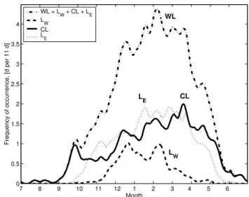
Fig. 2.Frequency of occurrence of the Winter Lows (WL) and their
components: cold Lows to the west (LW), Cyprus Lows (CL), and
Lows to the east (LE), for 1948–2003.
2 The Eastern Mediterranean Winter Lows’ seasonal
course
2.1 The Winter Lows’ course and comparison with earlier studies
Earlier studies on the multimodality in the EM emphasized the rainfall in one or several stations in Israel (Stiefel, 1981; Ronberg, 1984; SR88; Kutiel, 1985). SR88 pointed out the close relationship of the rainfall multimodality with the num-ber of the Cyprus Lows (CL) hitting the region as well as with the frequency of the upper troughs (Jacobeit, 1988) and the surface humidity of several stations in Israel. The monthly resolved seasonal variability of cyclonic activity is described by Alpert et al. (1990).
The current methodology of daily classification allows lo-cating the exact dates for the maxima and minima in the cy-clonic activity (Fig. 1). The Winter Lows’ group include all types of Mediterranean Lows (Fig. 2) migrating eastward via the EM, as in the example shown in Fig. 3 (Sect. 2.2). Fig-ure 4 compares between the dates in the cyclonic activity for two 28-yr periods (Sect. 2.3.2), and Fig. 5 focuses on the Cyprus Lows, the most important component of the Winter Lows.
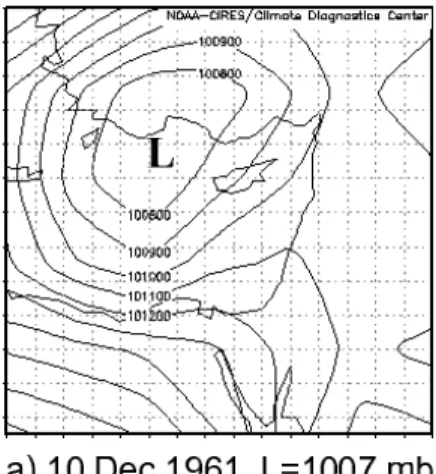
Fig. 3.Example of an Eastern Mediterranean winter spell. Daily sea level pressure successive maps for 10–14 December 1961 at 12:00 UTC:
(a)Lows to the west (LW),(b–d)Cyprus Lows (CL), and(e)Lows to the east (LE). Maps from NCEP/NCAR reanalysis at http://www.cdc.
noaa.gov.
resulting from the active surface Red Sea Trough combined with the upper trough and considered next (Sect. 2.3.4 and Sect. 3).
7 8 9 10 11 12 1 2 3 4 5 6 0
0.5 1 1.5 2 2.5 3 3.5 4 4.5
Month Frequency of occurrence, [d per 11d] Max I Max III
(a) L
W
(a)
Max II−III
Max IV−V
Max VI
(b)
(b) CL+L
E
I half: 1948−1975 II half: 1976−2003
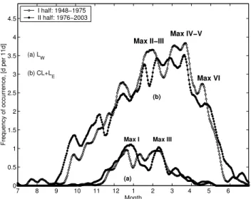
Fig. 4.Frequency of occurrence of the Winter Lows’ components:
(a)cold Lows to the west (LW)and(b)Cyprus Lows (CL) + Lows
to the east (LE), compared for 1948–1975 (open circles) and 1976–
2003 (black circles).
spring maximum Max VI (magnitude of 2.5 d/(11 d)) reaches up to 56% of the winter Max III.
Table 1a and Fig. 2 reveal some remarkable features of the WL seasonal course. The Max III seems to be a sym-metrical center with regards to the secondary extremes. Ta-ble 1a shows that for the first half of winter, every minimum is closer to the previous maximum (with a distance of only about 1 to 1.5 weeks), while in the second half of winter, af-ter Max III, this relation is in the opposite direction, i.e. each minimum is closer to the following maximum. The Max VI fits well this pattern (Table 1a; Fig. 2).
The Fast Fourier Transform was applied to the un-smoothed WL frequency of occurrence for the 128-day pe-riod from 16 December to 22 April. The pepe-riodicities of 44 to 7.5 days were found (Table 2). The dominant periodic-ity P2, of 22 days, fits a similar analysis by Sharon (1990)1 for rainfall. Sharon found the first harmonic of 24–25 days from February to April and fluctuation of 18–22 days from October to mid-December. The similar results for the two independent data-bases (synoptics and rainfall) support this frequency result.
The common 22- and 7.5-day periodicities (Table 2) for the two 28-yr periods confirms the same timing (assuming the same phase) in the course of the WL during a year, and consequently in the EM rainfall course.
2.2 Components of the Winter Lows’ group
Figure 3 shows a typical sequence of the WL spell days over the EM; each is characterized by cyclonic activity in some parts of the EM.
1Sharon, D.: Further study of intra-seasonal variations in rainfall
(personal communication), 1990.
7 8 9 10 11 12 1 2 3 4 5 6
0 0.5 1 1.5 2
[d per 11 d]
(a) CL I half: 1948−1975
II half: 1976−2003
7 8 9 10 11 12 1 2 3 4 5 6
0 0.5 1 1.5 2
Month
[d per 11 d]
(b) L
E
I half: 1948−1975 II half: 1976−2003
Fig. 5.Frequency of occurrence of the Winter Lows’ components:
(a)Cyprus Lows (CL) and(b)Lows to the east (LE), compared for
1948–1975 (open circles) and 1976–2003 (black circles).
Table 2.Periodicities (days) in the course of the WL frequency of
occurrence for 16 December–22 April.
Period P1 P2 P3 P4 P5 P6 P7
Full 44 22 16 13 11 9.4 7.5
I half 44 22–25 11 7.5
II half 33 22 16 13 9.4–10 7.5
WL = Winter Lows.
Full = full period, 1948–2003. I half = first half period, 1948–1975. II half = second half period, 1976–2003.
The cold Low to the west (LW)(Fig. 3a) is a deep low-pressure system often generated over N. Italy and located west to Cyprus. In this situation, it is common that N. Egypt, Cyprus and SE Turkey become rainy.
A Cyprus Low is obtained when a LWmoves eastward and is located near Cyprus, usually to the northeast of it. A cen-ter of the low pressure stays over the Cyprus area for several days, varying slightly in position and depth (Fig. 3b–d). Usu-ally Israel, Lebanon, Syria, and SE Turkey are favourable for rain (Fig. 3b), but sometimes N. Egypt (Fig. 3c), or Israel, Lebanon, Syria, and N. Egypt together (Fig. 3d).
Fig. 6.Example of a transition Sharav Low→Cyprus Low→Low to the east. Daily sea level pressure successive maps for 15–19 March
1998 at 12:00 UTC:(a)Sharav Low (SL),(b–d)Deep Cyprus Lows (CL), and(e)Lows to the east (LE). Maps from NCEP/NCAR reanalysis
at http://www.cdc.noaa.gov.
2.3.1 First factor – Cold Lows to the west
The LW are connected to Max I and Max III (Figs. 1, 2; Ta-ble 1). Their frequency peaks up to the value of 1 d/(11 d) twice a year, on 19–23 December and on 9–10 February, and drops in between, i.e. in January, by 40%, to 0.6 d/(11 d), see Fig. 2. In general, the frequencies of the LW during the cool season seem to be opposite to those in N. Italy based on the average monthly distribution of rainy days from where a
between west and east Mediterranean, the Mediterranean os-cillation as first described by Conte et al. (1989) and later by Kutiel et al. (1996). All this holds for both 28-yrs periods (Fig. 4a). The LW maxima are on the 20–21 December and 1–12 February for 1948–1975 and on the 22–30 December and 18–19 February for 1976–2003.
2.3.2 Second factor – stay over Cyprus
The EM synoptic cyclones placed over Cyprus area are of-ten delayed. This is due to the local topography of S. Turkey and Lebanon, heat and moisture fluxes from the sea surface (Alpert and Warner, 1986; Alpert et al., 1995), and cold con-tinental polar air masses from Russia or southeast Europe (Barry and Chorley, 2003). An example is given in Fig. 3. The LW position usually lasts only 1 day and is followed by a series of CL+LEdays. As pointed above, we define the Cyprus Lows when mainly the northern and central parts of the EM get rainfall, and Lows to the east when it holds for the central and southern parts. Since this division has been somewhat conventional, and there are cases classified as be-longing to CL while being only by a bit more distant of the LE cases (Alpert et al., 2004a) and vice versa, we will con-sider a total of the CL and LE frequencies a contribution of delay into the EM cyclonic activity (Fig. 4b).
A first “CL+LE” maximum is on 15 December for both 28-y half periods. This date is 3 days earlier than Max I (18–19 December, Table 1a) and reaches up to 2.8 d/(11 d) and 2.4 d/(11 d) for 1948–1975 and 1976–2003, respectively. Later, this sum rises very slowly up to 3.7 d/(11 d) by Max V for full period. The LE frequencies remain nearly constant during mid-January – early March, whereas the CL’s tend to increase (Fig. 2). It is notable from Fig. 5a that, in spite of the larger magnitudes of the CL peaks for 1948–1975 when the NAO was weak, the timing of the peaks is nearly the same for both 28-y periods.
2.3.3 Third factor – Sharav Lows
Additional sources for the Max V on the 19–20 March (Fig. 2 and Table 1a) are the Sharav Lows (SL). These synoptic sys-tems originate from the NE Africa. In March, due to a winter upper trough still presented over the EM, the Sharav Lows continue directly northward from NE Egypt to the Cyprus area and become Cyprus Lows. On the 19–20 March, Max V (Table 1a), the rising frequency of SL becomes about dou-ble the decreasing LW frequency (Fig. 2). A famous exam-ple was the deep low-pressure spell on 15–19 March 1998 (Fig. 6; Alpert and Ganor, 2001). A SL loaded the desert dust over the EM and then turned out into a deep CL. The latter stayed over Cyprus for 3 days and afterwards moved eastward, then delayed further as a LEfor 2 more days. The case resulted in heavy rains and mountainous snow.
7 8 9 10 11 12 1 2 3 4 5 6
0 0.5 1 1.5 2 2.5 3 3.5 4 4.5
RST: 1948−1975 ( I, narrow lines) and 1976−2003( II, wide lines)
Month
Frequency of occurrence, [d per 11 d]
RST
E: I
RST
E: II
RST
C: I
RST
C: II
RSTW: I RST
W: II
RST
C
RSTW RST
E
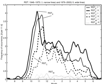
Fig. 7. Frequency of occurrence of the Red Sea Troughs (RST)
by subtypes: RST with the eastern, central, western axis (RSTE,
RSTC, and RSTW, respectively), compared for 1948–1975 (narrow
lines) and 1976–2003 (wide lines).
2.3.4 Fourth factor – RST
A secondary peak of the Winter Lows in early November (Fig. 1) is mostly accounting for the Lows to the east whose November peak is especially notable for 1976–2003 (Fig. 7, detailed next). In about 10% of the Red Sea Trough cases, a northern part of a surface RST from the south becomes as-sociated with an upper-tropospheric trough from the north, producing a Cyprus Low. Later, a Low to the east develops along with floods, mostly in the southern part of Israel (Ka-hana et al., 2004). During this period, WL spells enduring up to 6 days, are generated. Figure 2 shows that the LEin early November is frequent as about twice CL. Early November is the only period in the course of a year that such a relation between CL and LEexists, i.e. LE(%)≈2 CL(%). This holds for both climatologically significant periods of 1948–1975 and 1976–2003 (Fig. 5). The RST peak itself is discussed in detail next.
3 Calendaricities in the Red Sea Troughs
In this section, it will be shown for the first time that a sig-nificant bimodality exists in the seasonal course of Red Sea Trough. The RST frequency has a main peak in mid-autumn and a secondary peak in the winter.
in late October. Then, the RST frequencies keep on high level during 2 to 3 weeks, until about mid-November. The major maximum in the RST frequency in late October – early November is well-known by the EM meteorologists. Accord-ing to our daily data, the total RST frequency peaks on 2 to 15 November, in the middle of the EM autumn.
The major RSTE peak for 1976–2003 is on the 26 Octo-ber. For 1948–1975, there is a “step” around this date, on 30 October–2 November, reaching up to 94% of its peak that is on 13–14 November. It is remarkable that the magnitudes of the RSTEmaxima for two 28-y periods are very close to each other, having the values of 4.1 d/(11 d) and 3.9 d/(11 d), i.e. both around 4 d/(11 d).
The RSTC frequency peaks later than the RSTE by 1.5– 3 weeks: on the 24 November for first half period, 1948– 1975, and on 17 November for the second one, 1976–2003. The magnitudes of the RSTCmaxima are 2 and 3.2 d/(11 d), respectively. These results are the first evidence that RSTE are more frequent than RSTC. The RSTW frequencies are very low, but they appear in the same time span, from mid-October through April, for both half periods.
The probability of rainfall followed by floods is higher for RSTC than for RSTE. Hence, given the RSTE inten-sity reaching up 35%, on average, of the daily situations in late October and the RSTC’s – 22%, on average, in mid-November, there are two adjacent dates with the very high probability of the autumn floods: the end of October, and mid-November. Between these dates, the probability of floods remains high. The flood period lasts 2–3 weeks in the mid-autumn and separates the early dry and the late dry autumn.
The total RST frequencies (not shown) are peaking in the early November for both 28-y periods. This is in spite of the clear differences between the RST frequency’s magni-tudes for two 28-yr periods. The pronounced increase of the total RST frequencies for 1976–2003 at almost every cal-endar day, as compared to 1948–1975, explains the recent significant increase in the annual RST frequency. Alpert et al. (2004a) noted the nearly doubling in the average annual RST frequency from about 50 days in the 1950s to about 100 days in the 1990s. This could be associated with the recent rainfall decrease over most of the EM since RST is mainly associated with dry weather and winds from the eastern sec-tor. It is interesting to note that the contribution of the RSTC to the total RST increase is dominant during the autumn and early winter while later (late winter and spring) it is the RSTE that becomes the major contributor.
The difference between the magnitudes of the November RSTC maxima for two 28-yr periods is especially interest-ing: 3.2 d/(11 d) for 1976–2003 as compared to 2 d/(11 d) for 1948–75, that means 1.6 times increase. It explains the in-creased frequency of the catastrophic floods in S. Israel in the last decades (Kahana et al., 2004). In addition, as mentioned above, the November RSTC maxima for the second half pe-riod falls on 17 November that is by 1 week earlier then for
the first half (24 November). It explains why for 1976–2003, the floods peaked on average by one week earlier then for 1948–1975.
The more frequent the RST the more in its absolute value a small rain-bearing proportion of the RST. This paradoxical reduction in total rain while increase in heavy is the topic of the paper by Alpert et al. (2002). Here, we suggest an expla-nation (at least partly) based on increase of RST situations for the EM.
4 Conclusions
The E. Mediterranean winter season is shown to be multi-modal. The Winter Lows’ frequencies have the main peak on the 6 February, in midwinter, and secondary maxima on 18–19 December, 19 January, 1 March, 20 March. There is also a pronounced spring WL maximum on 19 April. The five maxima of the winter cyclonic activity, centered on early February, are nearly bell-shaped over their magnitudes.
The Winter Lows produce the rainfall over the central and northern EM areas, including Cyprus, Israel, Lebanon, NW Syria, W. Jordan. The southern EM areas, i.e. S. Israel and NE Egypt, get rainfall followed by floods due to the Winter Lows as well, and in addition, due to a small proportion of the mostly dry Red Sea Troughs that occasionally turn out to cause heavy rainfall. The EM autumn synoptic system of the Red Sea Trough has one main peak in early November. This time has the highest probability for the catastrophic floods in the southern part of the EM.
Appendix A
List of acronyms
CL Cyprus Lows
DJF December, January, February
EM Eastern Mediterranean
IPCC Intergovernmental Panel on Climate Change
LE Low to the east
LW cold Low to the west
Max maximum frequency
NAO North Atlantic Oscillation
NCAR National Center for Atmospheric Re-search
NCEP National Center for Environmental Pre-diction
NE northeast
NH Northern Hemisphere
NW northwest
RST Red Sea Trough
RSTE, RSTC, RSTW
RST with the eastern axis, axis over the coast, western axis, respectively (with respect to the EM eastern coastline)
SE southeast
SL Sharav Lows
UTC Universal Time Co-ordinated, also known as Greenwich Meridian Time (GMT)
WL Winter Lows
Acknowledgements. This study was partly supported by the GLOWA-Jordan River grant of the Ministry of Science Culture and Sport, Israel and the Bundesministerium f¨ur Bildung und Forschung (BMBF). The NCEP Reanalysis data were provided by the NOAA-CIRES Climate Diagnostics Center, Boulder, Colorado, USA, from their Web site at http://www.cdc.noaa.gov/. We are especially thankful to D. Sharon, of the Hebrew University of Jerusalem, for providing us with much detail on earlier studies.
Edited by: A. Mugnai Reviewed by: two referees
References
Alpert, P. and Ganor, E.: Sahara mineral dust measurements from TOMS – Comparison to surface observations over the Middle East for the extreme dust storm, 14–17 March 1998, J. Geophys. Res., 106, 18 275–18 286, 2001.
Alpert, P. and Warner, T. T.: Cyclogenesis in the Eastern Mediter-ranean, WMO/TMP Report Series, 22, 95–99, 1986.
Alpert, P., Neeman, B. U., and Shay-El, Y.: Intermonthly variability of cyclone tracks in the Mediterranean, J. Climate, 3, 1474–1478, 1990.
Alpert, P., Stein, U., and Tsidulko, M.: Role of sea fluxes and topography in eastern Mediterranean cyclogenesis, The Global Atmosphere-Ocean System, 3, 55–79, 1995.
Alpert, P., Osetinsky, I., Ziv, B., and Shafir, H.: Semi-objective clas-sification for daily synoptic systems: application to the Eastern Mediterranean climate change, Int. J. Climatol., 24, 1001–1011, 2004a.
Alpert, P., Osetinsky, I., Ziv, B., and Shafir, H.: A new seasons defi-nition based on the classified daily synoptic systems: an example for the Eastern Mediterranean, Int. J. Climatol., 24, 1013–1021, 2004b.
Alpert, P., Ben-Gai, T., Baharad, A., Benjamini, Y., Yeku-tieli, D., Colacino, M., Diodato, L., Ramis, C., Homar, V., Romero, R., Michaelides, S., and Manes, A.: The paradox-ical increase of Mediterranean extreme daily rainfall in spite of decrease in total values, Geophys. Res. Lett., 29(11), 1536, doi:10.1029/2001GL013554, 2002.
Barry, R. G. and Chorley, R. J.: Atmosphere, weather and climate, Routledge, 421 pp., 2003.
Brier, G. W., Shapiro, R., and Macdonald, N. J.: A search for rain-fall calendaricities, J. Atmos. Sci., 20, 529–532, 1963.
Conte, M., Giuffrida, S., and Tedesco, S.: The Mediterranean Os-cillation: impact on precipitation and hydrology in Italy, in: Pro-ceedings of Conference on Climate and Water, V. 1, Publ. of Academy of Finland, Helsinki, 121–137, 1989.
Duncan, R. A., Rao, M. S., and Lokanadham, B.: The reality of calendaricities in Indian rainfall, J. Atmos. Terr. Phys., 27, 1055– 1058, 1965.
Elbashan, D.: Monthly rainfall isomers in Israel 1931–1960, Israel J. Earth Sci., 15, 1–7, 1966.
Folland, C. K., Karl, T. R., Christy, J. R., et al.: Observed climate variability and change. Climate Change 2001: The Scientific Ba-sis, edited by: Houghton, J. T., Ding, Y., Griggs, D. J., et al., Cambridge Univ. Press, 99–181, 2001.
Godfrey, C. M., Wilks, D. S., and Schultz, D. M.: Is the January Thaw a statistical phantom?, Bull. Amer. Meteorol. Soc., 83, 53– 62, 2002.
Goldreich, Y.: Regional variation of phase in the seasonal march of rainfall in Israel, Israel J. Earth Sci., 25, 133–137, 1976. Jacobeit, J.: Intra-seasonal fluctuations of mid-tropospheric
circula-tion above the eastern Mediterranean. Recent Climatic Change: A regional Approach, edited by: Gregory, S., Belhaven Press, Ch. 8, 1988.
Kahana, R., Ziv, B., Dayan, U., and Enzel, Y.: Atmospheric predic-tors for major floods in the Negev desert, Israel, Int. J. Climatol., 24, 1137–1147, 2004.
Kalnay, E., Kanamitsu, M., Kistler, R., et al.: The NCEP/NCAR 40-Year Reanalysis Project, Bull. Amer. Meteorol. Soc., 77, 437– 471, 1996.
Katznelson, J.: Rainfall in Israel as a basic factor in the water budget of the country, Meteorological Papers, A24, Israel Meteorol. Ser. (in Hebrew), 1968.
Kutiel, H.: The multimodality of the rainfall course in Israel, as reflected by the distribution of dry spells, Archives for Meteorol-ogy, Geophys., and Bioclimatol., B36, 15–27, 1985.
Kutiel, H., Maheras, P., and Guika, S.: Circulation indices over the Mediterranean and Europe and their relationship with rainfall conditions across the Mediterranean, Theor. Appl. Climatol., 54, 125–138, 1996.
1998.
Maheras, P.: The synoptic weather types and objective delimitation of the winter period in Greece, Weather, 43, 40–45, 1988. Mapes, B. E., Liu, P., and Buenning, N.: Indian monsoon onset and
Americas midsummer drought: out-of-equilibrium responses to smooth seasonal forcing, J. Climate, 18, 1109–1115, 2005. Portig, W. H.: A search for rainfall calendaricities, J. Atmos. Sci.,
21, 462, 1964.
Ronberg, B.: An objective weather typing system for Israel: A syn-optic climatological study, PhD thesis, The Hebrew University of Jerusalem, 126 pp., 1984.
Sharon, D. and Ronberg, B.: Intra-annual weather fluctuations dur-ing the rainy season in Israel. Recent Climatic Change: A re-gional Approach, edited by: Gregory, S., Belhaven Press, Ch. 9, 1988.
Stiefel, S.: The Climate of Hafetz-Hayim 1970–1979. Israeli Min. of Agriculture (in Hebrew), 99 pp., 1981.
Weatherbase: http://www.weatherbase.com/, 2005.