Abstract
In this paper the effect of quadratic and cubic non-linearities of the system consisting of the crankshaft and torsional vibration damper (TVD) is taken into account. TVD consists of non-linear elastomer material used for controlling the torsional vibration of crankshaft. The method of multiple scales is used to solve the governing equations of the system. Meanwhile, the frequency response of the system for both harmonic and sub-harmonic reso-nances is extracted. In addition, the effects of detuning parame-ters and other dimensionless parameparame-ters for a case of harmonic resonance are investigated. Moreover, the external forces including both inertia and gas forces are simultaneously applied into the model. Finally, in order to study the effectiveness of the parame-ters, the dimensionless governing equations of the system are solved, considering the state space method. Then, the effects of the torsional damper as well as all corresponding parameters of the system are discussed.
Keywords
Crankshaft; non-linear vibrations; torsional vibration damper (TVD); multiple scales method; state space method.
Study on TVD parameters sensitivity of a crankshaft using
multiple scale and state space method considering quadratic and
cubic non-linearities
Nomenclature
b Crankshaft linear damping coefficient
c TVD linear damping coefficient
1
*
F Coefficient of excitation
2
*
F Coefficient of excitation
c
I Crankshaft polar mass moment of inertia
d
I TVD polar mass moment of inertia
c
k Crankshaft linear spring stiffness
d
k TVD linear spring stiffness
R. Talebitootia,* M. Morovati b
aAsst. Prof., School of Mechanical
Engineering, Iran University of Science and Technology, Tehran, Iran
e-mail: [email protected]
bM.Sc. graduated, School of
Automo-tive Engineering, Iran University of Science and Technology, Tehran, Iran e-mail: [email protected]
Latin American Journal of Solids and Structures 11 (2014) 2672-2695 2
k Crankshaft non-linear quadratic non-linearities
3
k TVD non-linear cubic non-linearities R Dissipated energy
t Dimensionless time T Kinetic energy V Potential energy
1
*
General coordinate system
2
*
General coordinate system
1
System natural frequency
Small dimensionless parameter
1
External excitation frequency
2
External excitation frequency
1
Detuning parameter
2
Detuning parameter
3
Detuning parameter
1 INTRODUCTION
The Vibration phenomenon is one of the most important issues should be treated to reduce the unpleasant shaking in various compartments. If the movement is left untreated, many consequent problems such as noise transmission into cavity of the car as well as fracture and failure of the compartments will be occurred. The crankshaft is one of those compartments should be attentioned. It is mostly manufactured with high mechanical strength cast iron. It should be strong enough to tolerate piston strokes without high torsion. In addition, it should be balanced very carefully to prevent vibrations generated from out of center weight of the crank.
Latin American Journal of Solids and Structures 11 (2014) 2672-2695 the crankshaft as well as possible vibrations of the ship’s structure due to the reaction force in the thrust bearings. Giakoumis et al. (2008) evaluated the crankshaft angular deformations during tur-bocharged diesel engine operation owing to the difference between instantaneous engine and load torques by the aid of an experimentally validated diesel engine simulation code.
Furthermore, many authors is applied multiple scales method to solve various kinds of partial differential equations (PDEs). Multiple Scales method is one of perturbation method branches which is aimed at finding approximate analytic solutions to problems whose exact analytic solutions cannot be found. The setting where perturbation methods are applicable is where there is a family of equations P
( )
e , depending on a parameter e1, and where P( )
0 has a known solution. Per-turbation methods are designed to construct solutions to P( )
e by adding small corrections toknown solutions of P
( )
0 . The singular aim of perturbation methods is to calculate corrections to solutions of P( )
0 . Perturbation methods do not seek to prove that a solution of P( )
0 , with correc-tions added, is close to a solution of P(e) for e in some finite range with respect to some measure of error. Its sole aim is to compute corrections and to make sure that the first correction is small with respect to the chosen solution of P( )
0 , that the second correction is small with respect to the first correction and so on, all in the limit when e approaches zero. R. Ghaderi and Azin Nejat (2014) is used multiple scales method to analyze the frequency response of Nano-Mechanical Canti-lever (NMC). Then, they applied the primary resonance excitations to show the softening phenom-enon in frequency response. Moreover, Eissa and Bassiouny (2003) is applied the method of multiple scales to construct a second order uniform expansion of the non-linear rolling response of a ship in regular beam seas.In most of analytical studies surveyed above, only one term is used to simulate the external force applied on crankshaft. The other external forces are neglected which may lead into improper results. In most of the researches, authors have not considered both inertia and gas forces in their model. These two terms are of high importance. In other word, if these are not modeled simultaneously could influence on crankshaft torsional vibration. In addition, the corresponding parameters of crankshaft and TVD are obtained with the aid of the FEM model developed in ABAQUS software and curve fitting method applied in a numerical procedure developed in MATLAB.
In this paper, nonlinear vibration of a crankshaft is studied using the multiple scales perturba-tion technique (MSPT) at harmonic and sub-harmonic resonance. The system consists of the main structure along with torsional vibration dampers. The external forces including both inertia and gas forces are simultaneously applied into the model. In order to study the effective parameters, the dimensionless governing equations of the system are solved, considering the method of state space in a steady state process. Then, the effects of the torsional damper as well as all corresponding param-eters of the system are discussed.
2 GOVERNING EQUATIONS OF THE SYSTEM
The governing equations of the system including the crankshaft and elastomer have been consid-ered. Therefore, in order to derive these equations a mathematical model is represented in this sec-tion, using rod and disk elements.
Latin American Journal of Solids and Structures 11 (2014) 2672-2695 Figure 1: Schematic model of rod and disk elements.
( ) i
i i i
d L L R
Q dt q q q
¶ -¶ +¶ =
¢ ¢
¶ ¶ ¶ (1)
*2 *2 *2 * * 2 * * 2 * * * 3 *
1 2 1 2 1 2 2 1 3 2 1
1 1 1 1
( ( ) ( ) ( ) )
2 c 2 d 2 c 2 d
L =T -V = I q¢ + I q¢ - kq + k q -q +
ò
k q -q dq +ò
k q -q dq (2)*2 * * 2
1 2 1
1 1
( )
2 2
R = bq¢ + cq¢ -q¢ (3)
where L is representing the difference between kinetic and potential energy, R is dissipated energy,
i
Q is external forces and qi is general coordinate system denoted as q1* and q2*.With substituting
Eqs. (2,3) into Eq. (1) the governing equations of the system are followed as:
* * * * * * 2 * * 3 * * * 2 * * * *
1 1 ( 2 1) 2( 2 1) 3( 2 1) 1 (2 1 ) 1sin 1 2sin 2
c c d
I q¢¢ +kq -k q -q -k q -q -k q -q +bq¢ -cq¢ -q¢ =F W +t F Wt (4)
* * * * * 2 * * 3 * * 2
2 ( 2 1) 2( 2 1) 3( 2 1) ( 2 1 ) 0
d d
I q¢¢ +k q -q +k q -q +k q -q +c q¢ -q¢ = (5)
where kc and kd are linear spring stiffness of the crankshaft and TVD respectively; Ic and Id are
polar mass moment of inertia of the crankshaft and TVD, respectively; k2 and k3 are non-linear quadratic and cubic Non-linearities of the crankshaft and TVD;band care linear damping
coeffi-cients of the crankshaft and TVD and * 1
F and F2* are the Amplitudes of the excitations. Also, in
Eqs. (4,5) it is assumed that * *
2 1 0
q -q > .
In order to get involve with standard equations, non-dimensional variables are introduced as follows:
* 1
t = wt , 1 1 1
c
K k I
w = + (6)
where t indicates the dimensionless time and w1 is the natural frequency of the system including
crankshaft and TVD.
Thus, Eqs. (4) and (5) are written as:
2 3
1 1 [ 2 2 1 1(1 2) b1(2 1) d1(2 1) (F1sin 1t F2sin 2t)
q +q + -e g q +zq +z q -q - q -q - q -q = e W + W (7)
2 2 3
2 ( 2 1) [ 2(1 2) b2( 2 1) d2( 2 1) ] 0
q +b q -q + -e z q -q + q -q + q -q = (8)
where e is a small dimensionless parameters and (.) represents the derivative with respect to t*
Latin American Journal of Solids and Structures 11 (2014) 2672-2695
є є є є є є
є є
2 2
2 1 2 1 2
1 1 1 2
* *
3 3 2 1 2
1 2 1 2
2 2
* *
1 2
1 2
1 2
, , , , ,
( )
, , , ,
( ) ( ) ( ) ( )
,
d c
c d c c d c d d c
c d c
c d d c d c c d c d
k b c c k k I
b b
k k I I I k k I k k
k k I k I F F
d d F F
k k I k k I k k k k k k
g x x x
w w w
b
w w
= = = = = =
+ + +
= = = = =
+ + + + +
W W
W = W =
(9)
3 SOLVING THE GOVERNING EQUATIONS
In this section the method of multiple scales proposed by Nayfeh and Mook (1995) is used to solve Eqs. (7,8). The approximate solution is represented followed as:
2
1( ; )t 10( ,T T0 1) 11( ,T T0 1) 12( ,T T0 1) ...
q e =q +eq +e q + (10)
2
2( ; )t 20( ,T T0 1) 21( ,T T0 1) 22( ,T T0 1) ...
q e =q +eq +e q + (11)
where e<<1, T0 and T1 are the fast and slow time scales defined as:
0
T =t, T1 =et (12)
In addition the time derivative becomes:
2
0 1 2 ...
d
D D D
dt = +e +e + ,
2
2 2 2
0 0 1 1 0 2
2 2 ( 2 ) ...
d
D D D D D D
dt = + e +e + + (13)
where Dn = ¶ ¶Tn.
Substituting Eqs. (10), (11) and (13) into Eqs. (7) and (8) and reconstructing the equation with respect to the power of e will result into two sets of equations:
The equations involving the zero order e0 can be written as:
2
0 10 10 0
D q +q = (14)
2 2 2
0 20 20 10 0
D q +b q -b q = (15)
The equations involving the first order e1 can be written as:
2 2 2
0 11 11 0 1 10 2 20 0 10 1 0 10 1 0 20 1 10 1 10 20 1 20
3 2 2 3
1 10 1 10 20 1 10 20 1 20 1 1 2 2
2 2
3 3 sin sin
D D D D D D b b b
d d d d F t F t
q q q g q z q z q z q q q q q
q q q q q q
+ = - + - - + + - +
- + - + + W + W (16)
2 2 2 2 2 3
0 21 21 0 1 20 11 2 0 10 2 0 20 2 10 2 10 20 2 20 2 10
2 2 3
2 10 20 2 10 20 2 20
2 2
3 3
D D D D D b b b d
d d d
q b q q b q z q z q q q q q q
q q q q q
+ = - + + - - + - +
- + - (17)
Latin American Journal of Solids and Structures 11 (2014) 2672-2695
10 A T1( )exp(1 iT0) A T1( )exp(1 iT0)
q = + - (18)
where A1 is a function of T1 at this level of approximation. Substituting Eq. (18) in Eq. (15) yields
the solution of q20 as:
20 A T2( )exp(1 i T0) A T3( )exp(1 iT0) cc
q = b + + (19)
where 2
(
2)
3 1 1
A =b A b - and cc stands for the complex conjugate of the preceding terms and A2
is an unknown function at this level of approximation. Substituting Eqs. (18) and (19) into Eq. (16) yields:
0
0 0 0 0 0
0 0 0 0
2
0 11 11 1 2 3 1 1 1 1 3 2 2 1 2
2
2 2
1 1 1 3 3 1 2 2 3 1 2
2 2
1 3 1 3 2 2 2 2 3 3 3 1 1
3 2
1 1 1 3
( 2 ) e ( )
e [( 2 ) e ( 2 2 ) e e 2 e
e 2 2 e 2 2 e e 2 2 ]
[( 3
iT
i T iT iT i T iT
i T i T i T iT
D iA A i A i A i A A i A
b A A A A A A A A A A
A A A A A A A A A A A A A
d A A A
b b
b b b
q q g z z z g bz
-
-¢
+ = - + - - + + +
+ - + + - +
-- - + + + + +
- - 0
0 0 0 0 0
0 0 0
0 0
3
2 3 2 2
3 1 3 1 1 1 1 3 1 3 1 2 2
2 2
2 2 2 2
1 3 3 2 2 3 3 3 3 1 1 2 1 2
2
2 2
1 1 2 1 2 3 1 2 3 2 2 2 3 3 2 1
2 1 2 3
3 ) e (3 6 3 6
6 6 3 3 )e 3 e e 3 e e
( 6 6 6 3 6 ) e 3 e e
6 e e
iT
iT iT i T iT i T
i T i T iT
iT i T
A A A A A A A A A A A A A
A A A A A A A A A A A A A A
A A A A A A A A A A A A A A A A A A A
b b b b b -+ - + - - + + - - + - -+ - + + - - +
+ 0 0 0 0 0 0
0 0 0 0 0 0 0 0
0 0 0 0 0 1 2
2 2 2
2 2
1 2 1 2 3 1 2
2 3 3 2 2 2 2 2 2
1 2 3 2 2 3 2 3 2 3
2 2
2 2
3 2 2 3 1 2
3 e e 6 e e 3 e e
6 e e e 3 e e 3 e e 3 e
e 3 e e 3 e e ] 0.5 e 0.5 e
iT i T i T iT iT i T
i T iT i T i T iT i T iT i T
iT i T iT i T iT i t i t
A A A A A A A
A A A A A A A A A A
A A A A F F NST
b b b
b b b b b
b b
- -
-- - - W W
+ + + +
- - -
-- - + + + +cc
(20)
where NST stands for terms that do not produce secular terms. Therefore, any particular solution of Eq. (20) contains secular or small divisor terms depending on the resonance conditions. The de-tuning parameters s1, s2 and s3 are introduced as follows:
1
2
b = +es , W = +1 1 es2, W = +2 2 es3 (21)
Substituting Eq. (21) in Eq. (20) and eliminating the terms that produce secular terms and small divisors in q11 yields the following expression:
2
1 2 3 1 1 1 1 3 1 1 2 1 1 1 2 3 1 1 1 1 1
2 2 2
1 1 1 3 1 1 3 1 3 3 1 2 3 3 1 1 3 3 1 1 2 2 1 1 3
1 2 1 2 3 1
2 2 exp( ) 2 exp( ) 3
6 3 3 6 6 6 3
0.5 exp( ) 0.5 exp( ) 0
iA A i A i A i A b A A i T b A A i T d A A d A A A d A A d A A d A A A d A A A d A A A d A A
F i T F i T
g z z z s s
s s ¢ - + - - + - + -+ - + + - - + + + = (22)
where the prime denotes the derivative with respect to T1 and also the overbar shows the complex
conjugate. The uniform solution of Eq. (20) can now be written as:
2 2
11 2 2 1 2 1 1 1 2 1 2 3 1 2 3 2 2 2 3 3
0 1 1 2 2 3 0
(1 / 1 )[ ( 6 6 6 3 6 )]
1
exp( ) ( )exp ( 1)
3
A i A d A A A A A A A A A A A A A A
i T b A A A A i T
q b g z b
b b
= - + - - + + -
Latin American Journal of Solids and Structures 11 (2014) 2672-2695 In Eqs. (23), the terms proportional to exp(2iT0), exp(2i Tb 0), etc are ignored, as these terms are neutral in resonance cases.
0 0
0
0 0 0 0
2 2 2 2
0 21 21 2 3 2 1 2 3 2 2 1 2
2
1 1 1 2 1 2 3 1 2 3 2 2 2 3 3 1 1 2 2 3
( 1) 2 2
2 2 2 1 1 1 1 2 2 3
2 e ( 2 ) e ( (1 ))[
( 6 6 6 3 6 )]e (1 3) ( )
e e [ e 2 ( 2 2 ) e e
i T iT
i T
i T i T iT iT
D i A iA i A i A A i A
d A A A A A A A A A A A A A A b A A A A
i A b A A A A A A A
b
b
b b
q b q b z z b b g bz
bz
-¢ ¢
+ = - + - + - + - +
- - + + - - -
-- - + + - + 0
0 0 0 0 0 0
0 0 0 0
0 0 0 0
2
1 3 3
2 2 2
1 2 1 3 1 2 2 3 2 2 2 3 2
3
3 2 2 2 2
3 3 2 1 1 3 1 3 1 1 1 3 1 1 3
2 2
2 2
1 2 1 2
( 2 )
e 2 e e 2 ( 2 2 ) e e e 2 2
e e 2 ] [( 3 3 )e (3 3 6 ) e
3( e e e e
i T
iT iT i T iT i T i T
iT i T iT iT
iT i T iT i T
A A A
A A A A A A A A A A A A A
A A d A A A A A A A A A A A A
A A A A
b
b b b
b b b - -+ - + - - + - + + + + + + - + + - -
-+ + 0 0 0 0 0
0 0 0 0 0 0
0 0 0 0 0 0 0
2 2
2 2
1 2 1 1 2 1 2
2 2 2 2
1 2 3 1 2 1 2 2 1 3 3 1 3 1 2 3
2 2 2 3 3 3 3 2
1 2 3 1 2 1 2 3 2 3 2 3
e e 2 e ) 3( e e
2 e e e e (2 2 ) e 2 e
2 e e e e 2 e ) e e 3
iT i T i T iT i T
iT i T iT i T iT i T
iT i T iT i T i T i T iT
A A A A A A A
A A A A A A A A A A A A A A A A
A A A A A A A A A A A A
b b b
b b b
b b b b
--
-+ + +
+ + + + + +
+ + - - - 0 0
0 0 0 0 0 0 0
0 0 0 0 0 0
2
2 2
2 2 2 2 2
2 3 2 2 2 3 2 2 3 3 3 3 2
2 2 2 2
2 3 3 2 3 2 3
e e
3 e e 3 e 3 e e ( 6 3 ) e 3 e
e 6 e 3 e e 3 e e ]
i T iT
i T iT i T i T iT iT iT
i T i T i T iT iT i T
A A A A A A A A A A A A A
A A A A A A A cc
b
b b b
b b b b
-
--
-- - - + - -
-- + + +
(24)
Substituting Eq. (21) in Eq. (24) and eliminating the terms that produce secular terms and small divisors in q21 yields the following equation as:
2 2 2
2 2 2 1 2 1 1 1 2 1 2 3 1 2 3 2 2 2 3 3
2
2 2 2 1 1 2 3 2 1 3 2 1 2 2 2 3 3
2 ( / 1 )[ ( 6 6 6 3 6 )]
( 6 6 6 3 6 0
i A A i A d A A A A A A A A A A A A A A
i A d A A A A A A A A A A A A A A
b b b g bz
bz ¢
- + - + - - + + -
-- + - + + - - = (25)
Now, it is convenient to introduce An in polar form as:
1
exp( ); 1, 2 2
n n n
A = a iy n = (26)
where an and yn are real components. Substituting Eq.(26) in Eqs. (22) and (25) and separating
real and imaginary parts yields the governing following equations:
3 2 3 2
1 1 2 1 1 1 1 1 2 1 1 2 1
1 2 2 3
3
0.5 (1 3 3 ) 0.75 (1 ) 0.5 (1 )cos
8 0.5 cos 0.5 cos
a a d a d a a b a a Z
F Z F Z
y¢ = - g G + - G + G - G + - G + - G
-
(27)
1 0.5 1 0.5 1 1 0.5 1 1 0.51 1 2(1 )sin 1 0.5 1sin 2 0.5 2sin 3
a¢ = - za + zaG - za - b a a - G Z + F Z + F Z (28)
2 2 2 3 3
2 2 2 2 1 2 1 1 2 2 2 1 2 2 2
3 3
0.5 0.75 ( 2 2 )
8 8
a a a a d d d d d d a d a
b y¢ = g G + G - G - + G - G + G - (29)
2 0.5 2( 2 1 )
a a
b ¢ = - b - + Gz z (30)
where:
1 2 1 2 1 1
Z = - y +y +sT , Z2 =s2 1T -y1, Z3 =s3 1T -y1,
2
2 1
b b
G =
- (31)
Latin American Journal of Solids and Structures 11 (2014) 2672-2695
4 HARMONIC RESONANCE
Considering the detuning parameters as b @2, W @1 1 and also taking the value of W2 far from 2, Eqs. (27-30) are written as:
3 2 3 2
1 1 2 1 1 1 1 1 2 1 1 2 1 1 2
3
0.5 (1 3 3 ) 0.75 (1 ) 0.5 (1 )cos 0.5 cos
8
ay¢ = - gaG + d a - G + G - G + d a a - G + b a a - G Z - F Z (32)
1 0.5 1 0.5 1 1 0.5 1 1 0.51 1 2(1 )sin 1 0.5 1sin 2
a¢ = - za + zaG - za - b a a - G Z + F Z (33)
2 2 2 2 2
2 2 1 1 1 2 2 2 1 2 2 2
3 3
0.5 0.75 ( 2 2 )
8 8
a d d d d d d a d a
by¢ = g G + G - G - + G - G + G - (34)
2 0.5 2( 2 1 )
a a
b ¢ = - b - + Gz z (35)
Steady state solutions of the system are obtained with considering an¢ =Zn¢ =0 in Eqs. (32-35)
simultaneously. From Eq. (35) it can be obtained that z2 = Gz1 . Using steady state condition in Eq. (31) results in:
1 2
y¢ =s , y2¢ =2s2 -s1 (36)
Thus, the steady state equations in this case are followed as:
3 2 3 2
2 1 2 1 1 1 1 1 2 1 1 2 1 1 2
3
0.5 (1 3 3 ) 0.75 (1 ) 0.5 (1 )cos 0.5 cos 0
8
a a d a d a a b a a Z F Z
s + g G - - G + G - G - - G - - G + = (37)
1 1 1 1 2 1 1 2
[z z(1 )]a b a a (1 )sinZ F sinZ 0
- + - G - - G + = (38)
2 2 2 2 2
2 1 1 1 2 2 2 1 2 2 2 2 1
3 3
0.5 0.75 ( 2 2 ) 2
8 8
a d d d d d d a d a
g G + G - G - + G - G + G - = s -s (39)
Using Eqs. (37-39), the frequency response equation of the system is constructed as:
2 2 2 2 2 2 2 2 2 2
1 1 1 1 2 1 2 1 1 1 2 2 1 1 1 2 1 2
2 3 2 3
2 1 1 1 2 1 2 1 1 1 1 1
2 2 2 2
1 2 1 2 1 1 1
( (1 )) (0.816 / ( )) ( )(3 6 2 3 6 3
3 3
8 4 ) [( (1 )) ] [ 2 (1 3 3 ) (1 )
4 2
(0.816 / ( )) ( )(3 6
F b a d d d d a d a d a d a d a d
a a a d a d a
d d d d a d a d
g
s s z z s g
+ - G G - G - G + - G - G - G + G
+ - = + - G + - - G + - G + G - G + - G
G - G - G + 2 2 2 2 2
2-2g2G -3a1G -d1 6a1Gd2+3a1Gd2+8s2-4 )]s1
(40)
5 SUB-HARMONIC RESONANCE
With assuming the detuning parameters as b @2, W @2 2 and also taking the value of W1 far from 1, Eqs. (27-30) are reconstructed as:
3 2 3 2
1 1 2 1 1 1 1 1 2 1 1 2 1 2 3
3
0.5 (1 3 3 ) 0.75 (1 ) 0.5 (1 )cos 0.5 cos
8
ay¢ = - gaG + d a - G + G - G + d a a - G + b a a - G Z - F Z (41)
1 0.5 1 0.5 1 1 0.5 1 1 0.51 1 2(1 )sin 1 0.5 2sin 3
a¢ = - za + zaG - za - b a a - G Z + F Z (42)
2 2 2 2 2
2 2 1 1 1 2 2 2 1 2 2 2
3 3
0.5 0.75 ( 2 2 )
8 8
a d d d d d d a d a
Latin American Journal of Solids and Structures 11 (2014) 2672-2695 Assuming the steady state conditions, Eqs. (41-43) are represented as:
3 3 2 2
3 1 1 2 1 1 1 1 2 1 1 2 1 2 3
3
0.5 ( 3 3 1) 0.75 (1 ) 0.5 (1 )cos 0.5 cos 0
8
a a d a d a a b a a Z F Z
s + G g + G - G + G - - - G - - G + = (44)
1 1 1 1 2 1 2 3
[z z (1 )]a b a a (1 )sinZ F sinZ 0
- + - G - - G + = (45)
2 2 2 2 2
2 1 1 1 2 2 2 1 2 2 2 3 1
3 3
0.5 0.75 ( 2 2 ) 2
8 8
a d d d d d d a d a
g s s
G + G - G - + G - G + G - = - (46)
Using the above equations (44-46), the frequency response equation of the system is followed as:
2 2 2 2 2 2 2 2 2 2
2 1 1 1 2 1 2 1 1 1 2 2 1 1 1 2 1 2
2 3 2 3
3 1 1 1 3 1 2 1 1 1 1 1
2 2 2 2
1 2 1 2 1 1 1
( (1 )) (0.816 / ( )) ( )(3 6 2 3 6 3
3 3
8 4 ) [( (1 )) ] [ 2 ( 1 3 3 ) (1 )
4 2
(0.816 / ( )) ( )(3 6
F b a d d d d a d a d a d a d a d
a a a d a d a
d d d d a d a
g
s s z z s g
+ - G G - G - G + - G - G - G + G +
- = + - G + - - G - - + G - G + G + - G
G - G - G + 2 2 2 2 2
2 2 2 3 1 1 6 1 2 3 1 2 8 3 4 )]1
d - gG - a G -d a Gd + a Gd + s - s
(47)
6 NUMERICAL METHODS
In order to numerically solve the system equations, they are written in non-dimensional state space forms. Therefore the four variables are defined as:
1 1, 2 1, 3 2, 4 2
y =q y =q y =q y =q (48)
The above equation can be written as follows:
1 2
y =y (49)
3 4
y =y (50)
Substituting equation (48) in dimensionless equations of system (7,8) results in below equations:
2 3
2 1 [ 2 3 2 1( 2 4) 1( 3 1) 1( 3 1) ] ( 1sin 1 2sin 2)
y +y + -e gy +zy +z y -y -b y -y -d y -y =eF W +t F Wt (51)
2 2 3
4 ( 3 1) [ 2( 2 4) 2( 3 1) 2( 3 1) ] 0
y +b y -y + -e z y -y +b y -y +d y -y = (52)
In other hand, with considering Eq. (48), the two second order dimensionless equations of the system are written in four first order dimensionless equations. These four equations are numerically solved in MATLAB software.
6.1 Linear torsional spring stiffness (kc) and non-linearity (k2) of the crankshaft calculation
Latin American Journal of Solids and Structures 11 (2014) 2672-2695
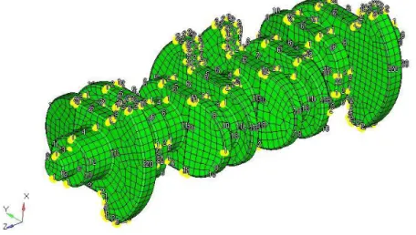
Therefore, the hexahedral meshes are devoted to this complex geometry of crankshaft. Then, the model is exported into ABAQUS software. The cast iron material with the properties as depicted in Fig. 2 is specified into the model. The crankshaft is cantilevered at the end and a 15 N.m torque is applied at the other side of crankshaft where the flywheel is placed. The main goal to apply the torque is to obtain the corresponding parameters of the crankshaft and TVD which is substantially independent to input applying torque. Therefore, the amount of input torque does not influence on the results of these corresponding parameters. Fig. 3 Shows isometric view of mesh elements of the crankshaft.
Characteristics Units Value
Diameter cm 2.7
Length cm 45.4
Number of fixed bearings --- 3 Number of movable bearings --- 4
Mass kg 13.2765
Volume cm3 1860
Table 1: General specifications of the crankshaft.
Figure 2: Stress-Strain Diagram of Cast Iron (Griswold and Stephens, 1987).
Figure 3: FE Model of the Crankshaft with High Precision Quads Mesh.
0 1 2 3 4 5 6 7
x 10-3 0
100 200 300 400
Strain
S
tre
s
s
(M
P
a
)
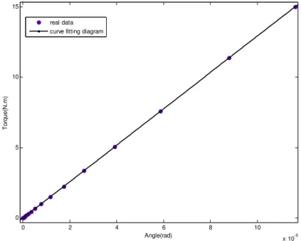
Latin American Journal of Solids and Structures 11 (2014) 2672-2695 Nonlinear analysis is chosen to model the stiffness factors. Therefore, the torque applied at the end of crankshaft; then it is plotted versus torsional angles as depicted in Fig. 4. It should be noted that the applications of numerical techniques in engineering often involve curve fitting of experi-mental data described by Mathews and Fink (1999). Therefore, a polynomials curve 2
2
c
k x +k x is
fitted into the simulated data. Consequently, the coefficients of stiffness factors could be extracted.
Figure 4: Curve Fitting 2 2
c
k x +k x to Crankshaft Torque.
The value of kc, k2 and their corresponding errors are listed in Table 2. The amounts of errors
listed in the Table are negligible which approve the values of stiffness parameters.
Value Units
Characteristics
129.2 kN.m/rad
c k
6.346 kN.m/rad
2
k
0 %
c k error
4.91 %
2
k error
Table 2: the values of stiffness parameters and their corresponding errors.
6.2 The torsional stiffness parameters of TVD model
Torsional vibration damper is applied to reduce the vibration in crankshaft. The TVD is placed at one side of crankshaft. It is known as a pulley placed on the crankshaft. It includes the different types of hub, rubber and ring components, as shown in Fig. (5).
0 2 4 6 8 10
x 10-5 0
5 10 15
Angle(rad)
T
o
rque(
N
.m
)
Latin American Journal of Solids and Structures 11 (2014) 2672-2695 a. Hub using quad mesh
b. Ring using quad mesh c. Rubber using quad mesh
Figure 5: Quad Meshing of Different Components of TVD.
Also, TVD components specifications are listed in Table 3.
TVD’s ring
specifications
TVD’s rubber specifications
TVD’s hub specifications
Inner diameter (cm) 12.17 10.87 10.56
Volume (cm3) 103 46.1 129
Mass (kg) 0.74 553x10-4 0.927
Mass moment of inertia (kg.m2) 307x10-5 179x10-6 141x10-5
Young’s modulus (kg/m.s2) 176x109 130x109 176x109
Poisson’s ratio (-) 0.25 0.27 0.25
Table 3: TVD’s specifications.
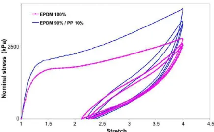
Then, considering TVD components into the model the analysis are performed similar as previous analysis discussed previously. There is a difference here and that the EPDM (Ethylene Propylene Diene Monomer) as depicted in Fig. 6. is specified for the rubber as well as cast iron which is speci-fied for the hub and ring components. The values of the torque applied into the system are plotted versus angle of crankshaft and then the stiffness factors are extracted in the same way as described before (Fig. 7).
6.3 Other component specifications
Latin American Journal of Solids and Structures 11 (2014) 2672-2695 Figure 6: EPDM Stress-Stretch Diagram (Bouchart et al. 2008).
Figure 7: Curve Fitting 3 3
d
k x +k x to TVD Torque.
The values of kd, k3 and their corresponding errors are shown in Table 4. The errors reported here
are also negligible.
Value Units
Characteristics
144400 kN.m/rad
d
k
3231 kN.m/rad
3 k
0 %
d
k error
5.23 %
3 k error
Table 4: The values of kd,k3and their corresponding errors.
0 1 2 3 4 5 6 7 8 9 10
x 10-8 0
5 10 15
Angle(rad)
T
or
que
(N
.m
)
Latin American Journal of Solids and Structures 11 (2014) 2672-2695
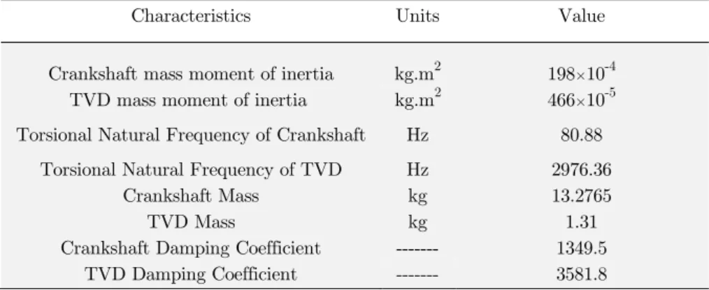
Characteristics Units Value
Crankshaft mass moment of inertia kg.m2 198×10-4
TVD mass moment of inertia kg.m2 466×10-5
Torsional Natural Frequency of Crankshaft Hz 80.88
Torsional Natural Frequency of TVD Hz 2976.36
Crankshaft Mass kg 13.2765
TVD Mass kg 1.31
Crankshaft Damping Coefficient --- 1349.5 TVD Damping Coefficient --- 3581.8
Table 5: Crankshaft and TVD specifications.
It is obvious from Table 5 that the amount of TVD damping coefficient is higher than crankshaft damping coefficient.
6.4 Excitation force
Mainly, the crankshaft vibrations originate among two principal sources from internal combustion engine. These sources contain the cylinder pressure as a first source. These also include the mass inertia of components caused from reciprocating movement of the piston. These two factors make the excitation function be more complicated. Fig. 8 shows the pressure excitation versus crankshaft angle with different terms. In addition, Fig. 9 shows the mass excitation moment of the engine components which are significantly influenced by engine rotation.
Figure 8: Engine Pressure Excitation Moment Diagram.
Figure 9: Engine Mass Excitation Moment.
0 100 200 300 400 500 600 700
-200 0 200 400 600
Crank Angle (Deg)
P
re
s
s
u
re
E
x
c
ita
tio
n
M
o
m
e
n
t (
N
.m
)
10 Terms Estimation
0 100 200 300 400 500 600 700
-150 -100 -50 0 50 100 150 200
Crank Angle (Deg)
M
a
s
s
E
x
c
ita
tio
n
M
o
m
e
n
t
(N
.m
Latin American Journal of Solids and Structures 11 (2014) 2672-2695
7 NUMERICAL RESULTS AND DISCUSSION
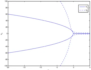
In some cases for designers it is so important to know the effect of varying design parameters on behavior of the vibration system. Therefore, in this section the effect of changing these parame-ters on vibration behavior of the system is presented. It should be noted that, dimensionless pa-rameters introduced depend on one or more physical papa-rameters of the crankshaft vibration be-havior. For instance, with improving the TVD linear damping coefficient, will lead into increasing the dimensionless parameter z1. In addition, enhancing the crankshaft linear damping coefficient will result in increasing the dimensionless parameter z . Moreover, with increasing the TVD line-ar spring stiffness the dimensionless pline-arameter g2 would be increased in this application. In a case of harmonic resonance from Eqs. (37-39) it should be considered the variation of an versus
the detuning parameter s2. Fig. (10) shows the variation of an versus s2 for real parameters
value. The bold lines represent crankshaft vibration amplitude versus detuning parameters in both unstable (curve) and stable (straight line) form. Also, the dotted lines represent TVD vibra-tion amplitude versus detuning parameter in both unstable (curve) and stable (straight line) form.
Figure 10: Variation of anVS Detuning Parameters2 for Real Parameters Value.
Figure. (11) Shows the effect of increasing dimensionless parameter z1 on response of the main system when it is 8 times greater than its real value. It is clear that increasing this dimensionless parameter leads to decreasing the curve inclination of crankshaft vibration and then becomes multi-valued at zone of steady state. In other words, the system status goes from unstable to sta-ble during the long time.
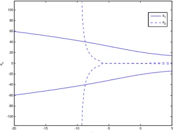
Figure (12) Shows the effect of increasing dimensionless parameter z on response of the main system when it is 15 times greater than its real value. It is clear that in this case by increasing this dimensionless parameter, the system tending to show more stable vibration than unstable vibration because of the value of detuning parameter. Also, by increasing this dimensionless pa-rameter, the crankshaft becomes completely multi-valued at zone of steady state but TVD be-comes single-valued at steady state zone.
-20 -15 -10 -5 0 5
-100 -80 -60 -40 -20 0 20 40 60 80 100
2
an
Latin American Journal of Solids and Structures 11 (2014) 2672-2695
Figure 11: the Effect of Increasingz1 on the Response of the Main System.
Figure 12: the Effect of Increasingz on the Response of the Main System.
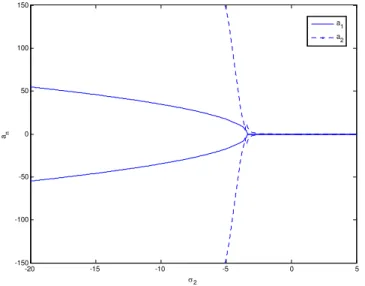
Figure. (13) Shows the effect of increasing dimensionless parameter g2 on response of the main system when it is 6 times greater than its real value. It is clear that in this case the system becomes stable during the minimum time. Also, by increasing this dimensionless parameter, the crankshaft amplitude at zone of transient is decreased and both crankshaft and TVD have single-valued at zone of steady state.
Figure (14) Shows the effect of increasing dimensionless parameter b on response of the main
system when it is 6 times greater than its real value. It is clear that the amplitude of vibration at transient zone is decreased and crankshaft has single-valued at zone of steady state. Also, the TVD has tending to have single-valued at zone of steady state.
Figure (15) Shows the effect of decreasing dimensionless parameter G on response of the main system when G = -0.33. In this case the behavior of the system is completely changed and both crankshaft and TVD shows divergence behavior. In addition, the system tends to be switched from steady (both dotted and bold straight) to unsteady (both dotted and straight curved) form.
-20 -15 -10 -5 0 5
-150 -100 -50 0 50 100 150
2
an
a1 a2
-20 -15 -10 -5 0 5
-100 -80 -60 -40 -20 0 20 40 60 80 100
2
an
Latin American Journal of Solids and Structures 11 (2014) 2672-2695 Figure 13: the Effect of Increasingg2 on the Response of the Main System.
Figure 14: the Effect of Increasing b1 on the Response of the Main System.
The non-dimensional equations of the system have been solved numerically in section 6. Now, in order to investigate the sensitivity of designing parameters of the system, the influence of pa-rameter variation on system behavior of crankshaft and TVD will be simulated graphically in a harmonic resonance case.
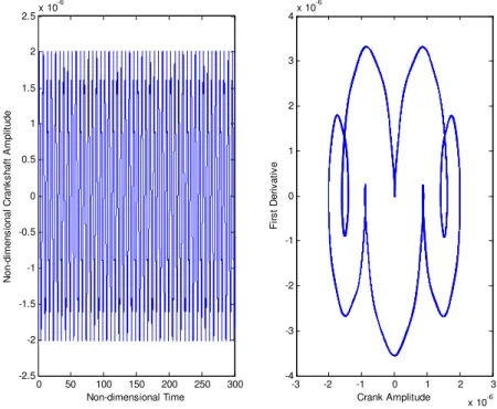
Firstly, the ratio of I2 I1 is assumed to be 0.1 of the case specified before. According to
Fig.(16,17), the crankshaft and TVD systems show different vibration behavior. In other word, the vibration amplitude of crankshaft is smaller than that of TVD system. This manner is a de-sirable case for dissipating the vibration energy, as the purpose of using TVD is to reduce vibra-tion amplitude of the system.
-20 -15 -10 -5 0 5
-150 -100 -50 0 50 100 150
2
an
a1 a2
-20 -15 -10 -5 0 5
-150 -100 -50 0 50 100 150
2
an
Latin American Journal of Solids and Structures 11 (2014) 2672-2695
Figure 15: the Effect of G on the Response of the Main System when G = -0.33.
Figure 16: Non-Dimensional Crankshaft Amplitude VS Non-Dimensional Time when (I2 I1)=0.1 and System Phase Diagram.
In Figs. (18,19), linear coefficients of crankshaft and TVD are 10 times of the reference case. It is well observed that, while the Non-dimensional time becomes 100, the amplitude of crankshaft and TVD with different vibration behavior approach into steady manner. Thus, two different zones in both diagrams called transient zone (Non-dimensional time is a value between 0 to 100) and steady state zone (Non-dimensional time is a value between 100 to 1000) are observed. In addition, the amplitude of TVD in steady state zone is a little lower than that of the crankshaft. However, with increasing linear coefficients of crankshaft and TVD to 10 times of their initial
0 50 100 150
-150 -100 -50 0 50 100 150
2
an
a1 a2
0 50 100 150 200 250 300
-2.5 -2 -1.5 -1 -0.5 0 0.5 1 1.5 2 2.5x 10
-6
Non-dimensional Time
N
on-di
m
ens
ional
C
rank
s
ha
ft
A
m
pl
it
ude
-3 -2 -1 0 1 2 3
x 10-6 -4
-3 -2 -1 0 1 2 3 4x 10
-6
Crank Amplitude
F
ir
s
t D
e
ri
v
a
ti
v
Latin American Journal of Solids and Structures 11 (2014) 2672-2695 values, the amplitude of crankshaft are considerably increased which leads into undesirable vibra-tion.
Figure 17: Non-Dimensional TVD Amplitude VS Non-Dimensional Time when (I2 I1)=0.1 and System Phase Diagram.
Figure 18: Non-Dimensional Crankshaft Amplitude VS Non-Dimensional Time when Linear Coefficients of Crankshaft and TVD are 10 Times and System Phase Diagram.
0 50 100 150 200 250 300
-5 -4 -3 -2 -1 0 1 2 3 4 5x 10
-6
Non-dimensional Time
N
o
n-di
m
en
s
ion
al
T
V
D
A
m
pl
it
ud
e
-5 0 5
x 10-6 -4
-3 -2 -1 0 1 2 3 4x 10
-6
TVD Amplitude
F
irs
t D
e
ri
v
a
ti
v
e
0 100 200 300 400
-3 -2 -1 0 1 2 3 4x 10
-3
Non-dimensional Time
N
on-di
m
ens
ion
al
C
rank
s
haf
t A
m
p
lit
ude
-4 -2 0 2 4
x 10-3 -1.5
-1 -0.5 0 0.5 1 1.5x 10
-3
Crank Amplitude
F
ir
s
t D
e
ri
va
ti
v
Latin American Journal of Solids and Structures 11 (2014) 2672-2695
Figure 19: Non-Dimensional TVD Amplitude VS Non-Dimensional Time when Linear Coefficients of Crankshaft and TVD are 10 Times and System Phase Diagram.
Figures (20,21) shows this negative effect of linear crankshaft damping on system vibration behavior. It should be noted that, when linear crankshaft damping is assumed negative about 25% from its real value, both crankshaft and TVD are tending to be unstable. In other words, the system has no desirable vibration behavior at all.
Figure 20: Non-Dimensional Crankshaft Amplitude VS Non-Dimensional Time with Negative Damping and System Phase Diagram.
0 100 200 300 400
-1.5 -1 -0.5 0 0.5 1 1.5x 10
-3
Non-dimensional Time
N
on-di
m
e
ns
ional
T
V
D
A
m
pl
it
u
de
-4 -2 0 2 4
x 10-3 -0.0005
-3.33e-4 -1.6e-4 0 1.6e-4 3.33e-4 0.0015
TVD Amplitude
F
irs
t D
e
ri
v
a
ti
v
e
0 50 100 150 200
-0.025 -0.02 -0.015 -0.01 -0.005 0 0.005 0.01 0.015 0.02 0.025
Non-dimensional Time
N
on-di
m
en
s
iona
l C
rank
s
haf
t A
m
pl
it
ude
-0.03 -0.02 -0.01 0 0.01 0.02 0.03 -0.03
-0.02 -0.01 0 0.01 0.02 0.03
Crank Amplitude
F
irs
t De
ri
v
a
ti
v
Latin American Journal of Solids and Structures 11 (2014) 2672-2695 Figure 21: Non-Dimensional TVD Amplitude VS Non-Dimensional Time with Negative Damping and System
Phase Diagram.
Figures (22,23) show the effect of neglecting damping ratio on vibration of the system. In this case, the crankshaft linear damping coefficient is reduced to 0.001. It is well depicted from these figures that both crankshaft and TVD behave in the same manner. In other word, their ampli-tude decreases during the non-dimensional time. Therefore, as a result of reduction of the system amplitude during the time and the tendency of the vibration amplitude of the system to zero, this reduction of crankshaft linear damping coefficient is desirable.
Figure 22: Non-Dimensional Crankshaft Amplitude VS Non-Dimensional Time with Linear Damping Coefficient Reduction and System Phase Diagram.
0 50 100 150 200
-0.2 -0.15 -0.1 -0.05 0 0.05 0.1 0.15
Non-dimensional Time
N
on-di
m
e
ns
io
n
a
l T
V
D
A
m
pl
it
ude
-0.2 -0.1 0 0.1 0.2
-0.08 -0.06 -0.04 -0.02 0 0.02 0.04 0.06 0.08
TVD Amplitude
F
ir
s
t D
e
ri
va
ti
ve
0 500 1000 1500 2000
-400 -300 -200 -100 0 100 200 300 400
Non-dimensional Time
N
on-di
m
e
n
s
iona
l C
ra
n
k
s
h
a
ft
A
m
pl
it
ud
e
-200 -100 0 100 200
-15 -10 -5 0 5 10 15
Crank Amplitude
F
ir
s
t D
e
ri
v
a
ti
v
Latin American Journal of Solids and Structures 11 (2014) 2672-2695
Figure 23: Non-Dimensional TVD Amplitude VS Non-Dimensional Time with Linear Damping Coefficient Re-duction and System Phase Diagram.
As depicted in Figs. (24,25), the effects of non-linear cubic TVD coefficients on vibration of the crankshaft and TVD are investigated .While non-linear cubic TVD coefficient is reduced to 0.001, crankshaft and TVD show the same vibration behavior. It is clearly observed that the sys-tem vibration amplitude is considerably high. In other word, the vibration of the syssys-tem is not desirable although the system having the steady state vibration during the broad band time.
Figure 24: Non-Dimensional Crankshaft Amplitude VS Non-Dimensional Time with Non-Linear Cubic TVD Coefficient Reduction and System Phase Diagram.
0 500 1000 1500 2000
-400 -300 -200 -100 0 100 200 300 400
Non-dimensional Time
N
on-d
im
ens
io
nal
T
V
D
A
m
pl
it
ude
-200 -100 0 100 200
-15 -10 -5 0 5 10 15
TVD Amplitude
F
irs
t D
e
ri
v
a
ti
v
e
0 500 1000 1500
-400 -300 -200 -100 0 100 200 300 400
Non-dimensional Time
N
on-di
m
ens
ional
C
rank
s
haf
t
A
m
pl
it
ude
-400 -200 0 200 400
-20 -15 -10 -5 0 5 10 15 20
Crank Amplitude
F
irs
t D
e
ri
v
a
ti
v
Latin American Journal of Solids and Structures 11 (2014) 2672-2695 Figure 25: Non-Dimensional TVD Amplitude VS Non-Dimensional Time with Non-Linear Cubic TVD
Coeffi-cient Reduction and System Phase Diagram.
8 CONCLUSION
In this paper the vibration behavior of a system consisting of crankshaft and TVD has been con-sidered. This system is described with second order non-linear differential equations. The method of multiple scales is applied to study the control of a combustion engine crankshaft vibration us-ing a non-linear elastomeric material vibration damper under the interaction of external excita-tions originated from different sources. Also, the numerical solution is applied to solve the non-dimensional equations of the system. Practically the following results are reported as:
The damping coefficient of the crankshaft could greatly influence on system behavior. The small or negative damping factor, leads into the worst behavior of the system, as it causes larger steady-states amplitudes or instability for both crankshaft and TVD.
Large magnitude of TVD non-linearities reduces TVD effectiveness.
While the ratio of (I2 I1) reduced to 0.1, the system behavior became steady. Therefore, this ratio is suggested in design process, if there are no other significant factors of limita-tion.
Linear Damping Coefficient Reduction leads into reduction of amplitude vibration in both crankshaft and TVD. This parameter is also very essential in designing the TVD for re-ducing the vibration of the whole system.
With increasing b1, the amplitude of vibration at transient zone becomes smaller. In
addi-tion, the crankshaft at steady state zone is single-valued.
As the magnitude of G has been taken the negative value, the system are going to be di-verged.
With increasing the g2, the crankshaft amplitude is decreased in transient zone. However, both crankshaft and TVD have single-value in steady state zone.
0 500 1000 1500
-400 -300 -200 -100 0 100 200 300 400
Non-dimensional Time
N
o
n-d
im
e
ns
io
na
l T
V
D
A
m
p
lit
ud
e
-400 -200 0 200 400
-20 -15 -10 -5 0 5 10 15 20
TVD Amplitude
F
irs
t D
e
ri
v
a
ti
v
Latin American Journal of Solids and Structures 11 (2014) 2672-2695
With increasing the z , the crankshaft becomes multi-valued in steady state zone. Howev-er, the TVD becomes single-valued in steady state zone.
While Non-Linear Cubic TVD Coefficient is reduced, both TVD and crankshaft show the same steady state behavior. However, the vibration amplitude of the system is considera-bly undesirable.
Acknowledgments
The authors would like to express their gratitude to the respected referees for many valuable comments which improve the presentation of this paper.
References
Asfar, K. R., (1992). Effect of Non-Linearities in Elastomeric Material Dampers on Torsional Vibration Control. International Journal of Non-Linear Mechanics 27: 947-954.
Bouchart, V., Bhatnagar, N., Brieu, M., Ghosh, A. K., Kondo, D., (2008). Study of EPDM/PP polymeric blends: mechanical behavior and effects of compatibilization. Comptes Rendus Mecanique 336:714-721.
Boysal, A., Rahnejat, H., (1997). Torsional Vibration Analysis of a Multi-Body Single Cylinder Internal Combus-tion Engine Model. Applied Mathematical Modeling 21: 481-493.
Eissa, M., El-Bassiouny, A. F., (2003). Analytical and numerical solutions of anon-linear ship rolling motion. Applied Mathematics and Computation 134: 243-270.
Esmaili, A. A., Khetawat, M. P., (1994). Dynamic Modeling of Automotive Engine Crankshaft. Mech. Mach. Theory 29: 995-1006.
Espindola, J., Bavastri, A., Lopes, M. O., (2010). On the Passive Control of Vibration with Viscoelastic Dynamic Absorbers of Ordinary and Pendulum Types. Journal of Franklin Institute 347: 102-115.
Ghaderi, R., Azin Nejat, A., (2014). Nonlinear mathematical modeling of vibrating motion of nanomechanical cantilever active probe. Latin American Journal of Solids and Structures 11: 369-385.
Giakoumis, E. G., Rakopoulos, C. D., Dimaratos, A. M., (2008). Study of Crankshaft Torsional Deformation under Steady-State and Transient Operation of Turbocharged Diesel Engines. International Mechanic Engineering 222: 17-30.
Griswold, F. D., Stephens, Jr. R. I., (1987). Comparison of fatigue properties of nodular cast iron production and Y-block casting. Int J Fatigue 413: 3-10.
Mathews, J.H., Fink, K,D., (1999). Numerical Methods Using MATLAB, Third Edition, Prentice Hall.
Montazersadegh, F. H., Fatemi, A., (2007). Dynamic Load and Stress Analysis of a Crankshaft. SAE Internation-al, 01-0258.
Mourelatos, Z. P., (2000). An Efficient Crankshaft Dynamic Analysis Using Substructuring with Ritz Vectors. Journal of Sound and Vibration 238: 495-527.
Mourelatos, Z. P., (2001). A Crankshaft System Model for Structural Dynamic Analysis of Internal Combustion Engine. Computers and Structures 79: 2009-2027.
Murawski, L., (2004). Axial Vibration of a Propulsion System Taking into Account the Couplings and the Bound-ary Conditions. Journal of Marine Science and Technology 9:171-181.