Temporal dynamics of hydrological threshold events

www.hydrol-earth-syst-sci.net/11/923/2007/ © Author(s) 2007. This work is licensed under a Creative Commons License.

Earth System

Sciences

Temporal dynamics of hydrological threshold events

G. S. McGrath1, C. Hinz1, and M. Sivapalan2

1_{School of Earth and Geographical Sciences, University of Western Australia, Crawley, Australia}

2_{Departments of Geography & Civil & Environmental Engineering, University of Illinois at Urbana-Champaign, USA} Received: 14 July 2006 – Published in Hydrol. Earth Syst. Sci. Discuss.: 1 September 2006

Revised: 6 February 2007 – Accepted: 6 February 2007 – Published: 26 February 2007

Abstract. The episodic nature of hydrological flows such as surface runoff and preferential flow is a result of the non-linearity of their triggering and the intermittency of rainfall. In this paper we examine the temporal dynamics of thresh-old processes that are triggered by either an infiltration ex-cess (IE) mechanism when rainfall intensity exceeds a spec-ified threshold value, or a saturation excess (SE) mechanism governed by a storage threshold. We use existing and newly derived analytical results to describe probabilistic measures of the time between successive events in each case, and in the case of the SE triggering, we relate the statistics of the time between events (the inter-event time, denoted IET) to the statistics of storage and the underlying water balance. In the case of the IE mechanism, the temporal dynamics of flow events is found to be simply scaled statistics of rainfall timing. In the case of the SE mechanism the time between events becomes structured. With increasing climate aridity the mean and the variance of the time between SE events increases but temporal clustering, as measured by the coef-ficient of variation (CV) of the IET, reaches a maximum in deep stores when the climatic aridity index equals 1. In very humid and also very arid climates, the temporal clustering disappears, and the pattern of triggering is similar to that seen for the IE mechanism. In addition we show that the mean and variance of the magnitude of SE events decreases but the CV increases with increasing aridity. The CV of IETs is found to be approximately equal to the CV of the magnitude of SE events per storm only in very humid climates with the CV of event magnitude tending to be much larger than the CV of IETs in arid climates. In comparison to storage the maximum temporal clustering was found to be associated with a max-imum in the variance of soil moisture. The CV of the time till the first saturation excess event was found to be greatest when the initial storage was at the threshold.

Correspondence to:Christoph Hinz chinz@cyllene.uwa.edu.au

1 Introduction

Many rapid hydrological processes such as runoff (Horton, 1933; Dunne, 1978), preferential flow (Beven and Germann, 1982), and erosion (Fitzjohn et al., 1998), are not continu-ous, but are triggered by thresholds. For example surface runoff occurs when the rainfall intensity is greater than the soils ability to adsorb it via infiltration. As a result some of these processes may even cease or are not even triggered if the rainfall event is too small. Because we consider rapid flow processes the duration of flow events is often small in comparison to the time between rainfall events. Therefore, what results from the threshold triggering, when we look at a time series, is a sequence of discrete, episodic events.

As the occurrence of these episodic processes is linked to the timing and magnitude of rainfall events it is natural therefore, to consider improving our understanding of how the temporal occurrence of these flow events relates to the structure of rainfall. This is the focus of this paper.

The temporal dynamics of preferential flow triggering due to between-storm and within-storm rainfall variability has been previously explored via the numerical simulation ap-proach, using synthetic rainfall time series (Struthers et al., 2007a,b). Struthers et al. (2007b) were able to relate aspects of the probability distribution function (pdf) and specific sta-tistical characteristics of the storm inputs to stasta-tistical prop-erties and aspects of the pdfs of preferential flow and runoff magnitude and timing. The analysis was not able to separate the contributions of the various runoff mechanisms to the sta-tistical properties of the resulting temporal flow dynamics. A simpler, more general approach was required to further de-velop the ideas presented in this work.

1982; Kung, 1990; Haria et al., 1994; Wang et al., 1998; Bauters, 2000; Dekker et al., 2001; Heppell et al., 2002), interception (Crockford and Richardson, 2000; Zeng et al., 2000), and hillslope outflow through subsurface flow path-ways (Whipkey, 1965; Mosley, 1976; Uchida et al., 2005; Tromp-van Meerveld and McDonnell, 2006). The storage threshold will be referred to here as saturation excess, al-though the use of this term is not often associated with some of the above processes.

In this article we examine the simplest possible conceptu-alizations for these two triggers. For infiltration excess we will use a threshold rainfall intensity (Horton, 1933; Heppell et al., 2002; Kohler et al., 2003) neglecting any soil mois-ture storage controls on the infiltration capacity. For satura-tion excess we use the opposite extreme, a threshold storage, depending only on the storm amount and not its intensity. While these two conceptualisations are very simplistic we expect a mixture of the results from these two processes to reflect more complex triggers, where triggering is a function of both rainfall intensity and storage.

The saturation excess mechanism captures the carry over of storage from one rainfall event to the next. As a result there is an enhanced probability that a second flow event will occur shortly after a flow event has just occurred because storage is more likely to be nearer the threshold in this inter-val. We hypothesize that this leads to temporal clustering of saturation excess, which means that multiple events occur in short periods of time separated by longer event-free intervals. A second aspect of the paper is to address the issue of ob-servability. For some processes we cannot measure directly the flux. Preferential flow is one such example. What we can observe of preferential flow is the timing of episodic pesti-cide leaching events (Hyer et al., 2001; Fortin et al., 2002; Laabs et al., 2002; Kjær et al., 2005) which are driven by this process. We also know that preferential flow is related to thresholds in soil moisture (Beven and Germann, 1982) and this can be measured reasonably well. For other processes, like subsurface hillslope outflow via soil pipes, the flux and timing might be observable but the internal, storage process much less so. There is clearly a need to better understand the inter-relationships between timing, flux, and storage in order to be able to make better predictions of these thresh-old processes where the internal dynamics are largely hidden (Rundle et al., 2006, this issue). In this paper it will be pos-sible to make this inter-comparison for the saturation excess trigger.

The paper begins with a brief overview of the simple mod-els of rainfall adopted for this analysis. Based upon this we derive analytically the statistics of the time between thresh-old events for infiltration excess and saturation excess mech-anisms, and for saturation excess we also present existing and newly derived statistics of the runoff flux based upon the original work of Milly (1993; 2001). Finally, we explore the results in the context of storm properties and the climate set-ting.

2 Rainfall models

For modelling purposes we adopt simple stationary descrip-tions of rainfall without any seasonal dependence. Storms are characterised only by three parameters, their total depth h [L], a maximum within-storm intensity Imax [L/T], and a time between stormstb [T]. Storms are considered to be instantaneous events, independent of one another, therefore satisfying the Poisson assumption as used commonly in hy-drology (Milly, 1993; Rodriguez-Iturbe et al., 1999). Such an assumption is considered valid at near daily time scales (Rodriguez-Iturbe and Isham, 1987).

As we are primarily concerned with an event based de-scription of processes, this rainfall model is appropriate to make direct comparisons between the process and its driver. Our objective is to capture the inter-(rainfall)-event dynam-ics, i.e. this event did or did not trigger the threshold and not the detail of within-event processes which is left for future research.

The Poisson assumption implies that the random time between storms, the inter-storm time, that results is de-scribed by an exponential probability density function (pdf) (Rodriguez-Iturbe et al., 1999):

gT b[tb]= 1 tb

e−tb/tb ₍₁₎

which is fully characterised by its meantb[T]. Storm depths are also assumed to follow an exponential pdffH[h] with a meanh[L]. The maximum within-storm rainfall intensity is also considered to be exponentially distributed with a mean ofImax[L/T].

Clearly this rainfall model is a gross simplification of real rainfall, particularly as it neglects seasonality. How-ever its advantage is it makes the later derivations analyti-cally tractable. Considering it’s use to describe within a sea-son rainfall may be more appropriate, but the statistics we will derive later may not necessarily reflect the transient dy-namics of storage in certain climates (Rodriguez-Iturbe et al., 2001). We also derive here statistics based upon an arbi-trary initial condition which may account for this transient behaviour.

3 Statistics of temporal dynamics

(a)

5 10 15 20 25 30 35

TimeHdaysL

20 40 60 80 100 120 140

I max

H

mm



day

L

Τ₁ Τ₂ Τ₃

(b)

2 4 6 8 10 12 14 16 18

TimeHdaysL

0 0.2 0.4 0.6 0.8 1. 12. 8. 4. 0.

Storage

s

Rainfall

mm

Τ₁ Τ₂ Τ₃

s0

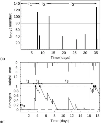
Fig. 1. Definition of the more general first passage timeτ1and the

inter-event timeτ2andτ3for(a)a threshold rainfall intensity

infil-tration excess (IE) trigger, where in this example intensities above

Iξ=80 mm/day trigger an IE event; and(b)a storage, or

satura-tion excess mechanism (SE), occurring whens₌1. The variables0

denotes the initial storage.

Fig. 1a and Fig. 1b. In the case of infiltration excess runoff, a flow event is triggered when the maximum rainfall intensity within a storm exceeds the infiltration capacity Iξ . Simi-lalry, when the soil water storage reaches a critical capacity a saturation excess event is deemed to have been triggered.

To quantify the pdfs of the first passage times and the IETs, we use the first four central moments. For completeness we define the moments in this section and will derive analytical expressions for them in Sect. 5.2 and A. The meanTµ [T] and thekt hcentral momentµk of the random variableτ are related to the pdfgT[τ] by the following (Papoulis, 2001):

Tµ=E[τ]= Z _∞

−∞

τ gT[τ] dτ (2)

µk=E h

(τ₋E[τ])ki= Z _∞

−∞

τ ₋Tµ k

gT[τ] dτ (3) for integers k _≥ 2, where E[ ] denotes the expectation operator. In addition to the mean and the varianceT_σ2=µ2 [T2], we will also use the dimensionless statistic, the coef-ficient of variation (CV), Tcv=

p

T_σ2T_µ [−], the ratio of

Table 1.Storm and infiltration excess inter-event statistics

Statistic Storm Infiltration excess

Tµ tb tbeIξ/Imax

T_σ2 t2_b

tbeIξ/Imax 2

Tcv 1 1

Tε 2 2

Tκ 6 6

the standard deviation to the mean, which gives a measure of the variability relative to the mean; the coefficient of skewnessTε=µ3µ2

3_/2

[₋], which describes the asymme-try of the probability distribution, where positive values in-dicate that the distribution has a longer tail towards larger values than smaller values; and the coefficient of kurtosis Tκ=µ4

µ22₋3 [−], where positive values indicate a more peaked distribution, in comparison to a normally distributed variable, and ”fatter tails” i.e. an enhanced probability of ex-treme values (Papoulis, 2001).

In order to compare the statistical properties of flow event triggers with the rainfall signal, we summarise here the rain-fall in terms of IET statistics. The idea here is to compare and contrast storm IET and flow IET statistics for the vari-ous threshold driven processes. Events which are temporally independent of one another have an exponential IET pdf. Ta-ble 1 lists the statistics for the storm IET.

A property of the exponential distribution is that the mean is equal to the standard deviation, and therefore the CV is equal to 1. The CV of the IETTcvis often used to distinguish temporally clustered and unclustered processes (Teich et al., 1997). Temporal clustering is said to occur whenTcv>1, aTcv=0 indicates no variability and exactly regular events, while aTcv<1 may indicate a quasi-periodic process (Wood et al., 1995; Godano et al., 1997).

4 Infiltration excess inter-event time statistics

This constant threshold filtering is the same as the rain-fall filtering described in Rodriguez-Iturbe et al. (1999) in the context of the soil water balance. They showed that a threshold filtering of the depth of rainfall with Poisson ar-rivals resulted in a new Poisson process. The rate of events over this threshold equalled the storm arrival rate multiplied by the probability of exceeding the threshold storm depth by a single event (Rodriguez-Iturbe et al., 1999). The differ-ence for the IE trigger considered here lies only in seman-tics. When the maximum within-storm rainfall intensityImax is exponentially distributed with meanImaxthe probability thatImax>Iξ is equal toe−Iξ/Imax and therefore the result-ing mean time between IE events is equal toT_µI₌tbeIξ/Imax. Table 1 lists the IET statistics that result.

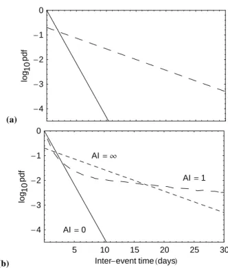
A soil withIξ=2Imaxresults in a mean IET which ise2 times longer than the mean storm IETtb, and a variancee4 times greater than the storm IET variancet2_b. The higher cen-tral moments remain unchanged. The IE filtering therefore results in temporal dynamics that are statistically the same as the rainfall’s, but scaled by a factor related to the single event probability of exceeding the threshold. This is illustrated in Fig. 2a, which is a semi-log plot of an example infiltration excess IET pdf, corresponding to the above example, shown in comparison to the rainfall IET pdf.

5 Saturation excess filtering

In this section saturation excess is described on the basis of Milly’s (1993) nonlinear storage-runoff model. Milly (1994) used this model to describe the impact of rainfall intermit-tency and soil water storage on runoff generation at catch-ment scales, and which he successfully used to capture much of the spatial variability in the annual water balance in catch-ments across much of continental USA. We use this mini-malist framework to model the triggering of runoff by the exceedance of a threshold value of storage. We first review his analytical results for the statistics of soil moisture stor-age and the mean water balance components. We then go on to derive from these results the variance of the saturation excess runoff flux on a per storm basis. We will later relate these statistics to those of the temporal dynamics of satura-tion excess triggering.

5.1 Storage and the water balance

Milly’s (1993) water balance model is represented in terms of a simple bucket with a fixed storage capacityw0[L] which wets in response to random storm events and dries in the inter-storm period, of random duration, due to a constant evaporative demandEm[L/T]. The threshold soil moisture (sξ=1 [-]) for flow initiation is assumed to have been reached when the store is filled to capacity. Any excess rainfall be-comes saturation excess. The resulting stochastic balance equation for water storages[-] (a dimensionless storage

nor-malised byw0) is: ds

dt= −L[s]+F[s, t] (4) wheret[T] denotes time,L[s] [T−1] the (normalised byw0) evaporative losses from storage. F[s, t] [−] denotes instan-taneous random infiltration events (normalised byw0), oc-curring at discrete timesti. Infiltration is limited by the avail-able storage capacity i.e. F[s, ti]=min1−s_i−, hiw0, wheres_i− [−] denotes the antecedent soil moisture andhi [L] the random storm depth. Evaporation losses are given by:

L[s]₌  



0 for s₌0

Em

w0 for 0<s ≤1

(5)

In this article we largely consider the transformation of Eq. (4) directly into the statistical properties of IETs, how-ever, we discuss briefly here how to numerically simulate a storage time series. This is done in part to help explain the conceptualisation of the process as well as to describe how we generated example time series presented in Sect. 6.3.1. Simulation involves generating a random storm IETtb and a subsequent storm depthhfrom their respective probability distributions. Storage at any timet in the inter-storm period can be calculated froms[t]=max [0, s0−Em(t−t0)/w0], wheret0is the time of the last storm when soil moisture was s0. At the end of the inter-storm periodti=t0+tbstorage im-mediately prior to the storm is given bys_i−. Storage increases froms_i−tos_i+₌min

1, s_i−₊h/w0due to the storm also at a time ti. This occurs as an instantaneous event with stor-age taking on two separate values immediately either side of timeti. The simulation is then continued withs_i+as the new s0and so on.

From the above model and the characteristics of rainfall presented before, two similarity parameters can be defined: the supply ratio α₌w0h, the ratio of storage capacity to mean storm depth, and the demand ratio β₌w0

Emtb

, the ratio of storage capacity to mean potential inter-storm evaporation (Milly, 1993). Whenα₌0 the rainfall supply is infinitely larger than storage capacity and whenα_=∞the supply is negligible compared to the amount in storage at capacity. Similarly β₌0 indicates infinite evaporative de-mand andβ_=∞negligible demand relative to the storage capacity. Typically one could expect the parameters to range from about 1 to 100 depending upon the process considered. For example a thin, near surface, water repellent layer with 10 mm of storage could have realisticα values of 1 to 10 depending upon the mean storm depth. Runoff controlled by storage throughout the rooting depth may have much larger values (Milly, 2001).

The ratioAI₌ Emtb h=α

aridity index (Budyko, 1974; Arora, 2002). AnAI <1 de-scribes a humid climate, Ai>1 an arid climate andAI₌1 defines equal mean rainfall and mean potential evaporation.

Milly (1993) derived the pdf of water storage in the form of two derived distributions of storage: one for a time im-mediately before a storm f_S−, the antecedent storage pdf, and one immediately after a stormf_S+. The pdf for storage for all timesfS, that resulted from that analysis was found to be equal tofS− (Milly, 2001). This was essentially be-cause storms were modelled as instantaneous events, with no duration, and the expected time of the next storm is an ex-ponential distribution emanating from a memoryless Poisson process for the rainfall arrivals. The pdf offS is given by (Milly, 2001):

fS=pβ e(α−β)s+qδ[s] (6) whereδ denotes the Dirac delta function, p describes the probability storage is at capacity (s=1), andqthe probability that the soil is dry (s₌0) and are given by:

p₌α−β

α eα−β (7a) q₌ β−α

β eβ−α_−α (7b) The resulting meanSµ[-] and varianceSσ2 [-] of storage

are given by Eq. (8) and Eq. (9) respectively (Milly, 2001): Sµ=

1 α₋β+

1+β eβ−α

β eβ−α_−α (8)

S_σ2=

1 (α₋β)2 −

1+(α₊2) β eβ−α

β eβ−α_−α2 (9) Based on the definition of the expected value of a func-tiong[x] of a random variablex , with a known pdffX[x] (Papoulis, 2001):

E[g[x]]₌ Z ∞

−∞

g[x]fX[x] dx (10) Milly (1993) derived the mean actual evaporationEa[L] per inter-storm period via:

Ea

h = w0

h Z 1

0−

L[s] fS[s] ds=1−

α₋β

α eα−β_−β (11) where the 0−is used to denote inclusion of the probability thats₌0.

From mass balance considerations Milly (1993) then de-termined the mean runoff per stormQµ[L] as follows:

Qµ

h =1− Ea

h =

α₋β

αeα−β_−β (12) Extending such analysis, we derive here for the first time the variance of flux per storm eventQ_σ2

L2which we cal-culate from the definition of the variance of a function of two

random variablesG[x, y] which have a joint pdffXY[x, y] (Papoulis, 2001) which is given by:

Eh(G[x, y]−E[G[x, y]])2i= Z ∞

−∞ Z ∞

−∞

(G[x, y]−E[G[x, y]])2fXY[x, y] dx dy (13) The magnitude of saturation excess generated on a single eventQi is given by:

Qihi, s_i−=max0, hi −w0 1−s_i− (14) which depends upon the two random variables, storm depth hi and the antecedent soil moistures_i−. As the pdf of soil moisture immediately prior to a rainfall eventfS− is equiv-alent to the pdf of soil moisturefS Eq. (6) in this instance (Milly, 2001) and ashands−_{are independent random} vari-ables we can apply Eq. (13) and the condition Eq. (14) to the calculation of the saturation excess runoff varianceQ_σ2 by

the following:

Q_σ2

h2 = Z 1

0− Z _∞

w0(1−s) _w0

h

_h

w0 −1+s

−Qµ h

2 ×

w0fH[h]fS[s] dhds + Z 1

0−

Z w0(1−s)

0

−Qµ

h 2

fH[h]w0fS[s] dhds

= (α−β) 2α e α−β

−α₋β α eα−β_−β2

(15)

The statistics of storage (Eq. 8, Eq. 9) and the flux (Eq. 12, Eq. 15) will be explored in more detail later on.

5.2 Statistics of saturation excess timing

For the type of stochastic process modelled by Milly (1993), Masoliver (1987) and Laio et al. (2001) provided derivations for the mean time to reach a threshold for the first time. This methodology was subsequently applied to describe the mean duration of soil moisture persistence between upper and lower bounds in order to investigate vegetation water stress (Ridolfi et al., 2000).

The mean FPT describes the expected waiting time till an event dependent upon the initial condition, of which the mean IET is a special case. The temporal dynamics also con-sists of the variability about this mean behaviour, therefore in Appendix A we present, for the first time, an extension of the derivation for the mean first passage time (Laio et al., 2001) giving a general solution to the higher moments of the FPT, such as the variance.

T_µs

s0, sξtill an arbitrary threshold storagesξis reached for the first time, when the initial storage wass0≤sξas:

T_µs s0, sξ tb =

α αesξ(α−β)_−βes0(α−β)

(α₋β)2 −

β α sξ −s0+1 α₋β (16) This is the same result, after appropriate adjustment of pa-rameters, as given by Eq. (31) in Laio et al. (2001). The mean saturation excess IETT_µs[1,1] comes from substitu-tion ofs0=sξ=1 in Eq. (16):

T_µs[1,1] tb =

αeα−β₋β

α₋β (17) As a result of our more general derivation we can use equations (A5), (A13) and (A10) together with n₌2, and T1₌T_µss0, sξ, to derive the raw moment T2. From the relationship between the central moments and the raw mo-ments (see Table A1), the FPT variance is calculated by Ts

σ2

s0, sξ=T2−T₁2. After substitution ofs0=sξ=1 we can show the variance of IET arising from the storage threshold, Ts

σ2[1,1] is given by:

Ts σ2[1,1]

t2_b =

2αβeα−β_(α +β₊2) (β₋α)2 +

(α₊β) β2₋α2e2(α−β) (β₋α)3 (18) In this paper we do not present the full solution for Ts

σ2

s0, sξ or the other higher moments as they are rather cumbersome; however complete solutions for the first four moments are provided as supplementary material (http://www.hydrol-earth-syst-sci.net/11/923/2007/ hess-11-923-2007-supplement.pdf). Table 2 summarises the first four central moments of the IET for three limiting cases, as discussed in more detail in the next section.

6 Results and Discussion

6.1 Climate controls on threshold storage events

This section discusses the analytical results for the statistical properties of the time between SE events and the statistics of the SE event magnitudes based on an investigation of three limiting climates: a super humid climate with an aridity in-dexAI₌0 by taking the limitα_→0 of the derived statistics; a super arid climate with an aridity indexAI_=∞by taking the limitβ_→0; and an intermediate climate withAI₌1 by taking the limitβ_→α. The analytical results corresponding to these limiting cases are summarised in Table 2.

6.1.1 Super humid climates:AI₌0

In very humid climates the temporal statistics of saturation excess IET are identical to that of the rainfall (see Table 2). This is because with an excess supply of rainfall and negli-gible evaporative demand the soil is always saturated. The statistics are consistent with an inter-event time which is ex-ponentially distributed. No filtering takes place as every rain-fall event triggers flow and all rainrain-fall becomes saturation excess (see Table 2). The rainfall signal is therefore an ex-cellent indicator of the timing, frequency and magnitude of SE events.

6.1.2 Super arid climates:AI_=∞

The IET statistics of SE events for an arid climate (Table 2) resemble those of the IE filtering described above (refer to Table 1). The average rate of SE events is scaled by the probability of filling the store completely in a single event i.e. byP[h>w0]=e−w0

h

=e−α. For example, consider a water repellent soil with a distribution layer which triggers finger flow after a critical water content (Dekker et al., 2001) equivalent to 10 mm of storage. In an extremely arid climate (β _≈0) withh₌2 mm (α₌5), andtb=5 days, the resulting mean and variance of the preferential flow IET is 5e5days and 25e10 days2respectively. Again the statistics are con-sistent with an IET which is exponentially distributed. The independence of events is maintained because soil moisture is completely depleted before every rainfall event. In this in-stance a simple filtering of the rainfall, forh>w0, provides a good predictor of the timing, relative frequency and magni-tude of storage threshold flow events.

The mean saturation excess magnitudeQµis also propor-tional to the mean storm depth scaled by the probability of filling the store on a single event (see Table 2). Unlike the simple threshold filtering, as described by the temporal dy-namics, the variance of the magnitude of saturation excess events per stormQ_σ2 is larger than would be expected for

an exponentially distributed random variable with the given mean. We believe this is due to the fact that the statistic in-cludes a large number of zero values where storms do not trigger a threshold storage event. A CV of event magnitude Qcv=

√

2eα_{−1 indicates that in the limit of a very arid} cli-mate the relative variability of the magnitude of these events increases with increasing storage capacity and decreasing storm depth (increasingα). For the example described above (α=5) the mean, variance and CV of event magnitudes are equal to Qµ=0.013 mm Qσ2=0.054 mm2 andQcv=17.2 respectively.

6.1.3 A balanced climate:AI₌1

Table 2.Summary statistics of the saturation excess inter-event times and event magnitudes in three limiting climates

Statistic Rainfall Humid Intermediate Arid

AI=0 AI=1 AI=∞

T_µs[1,1] tb tb tb(1+α) tbeα

Ts

σ2[1,1] t

2

b t

2

b 23 α3+2α2+2α+1

t2_b tbeα2 T_cvs [1,1] 1 1

√ 3 √

2

√

α3_+2α2_+2α+1

1+α ≥1 1

T_εs[1,1] 2 2

√

3 4α5_+20α4_+40α3_+45α2_+30α+10

5√2α(α(α+3)+3)+3 ≥2 2 T_κs[1,1] 6 6 B1α7+B2α6+B3α5+B4α4+B5α3+B6α2+B7α+B8

35(2α(α(α+3)+3)+3)2 −3≥6

a ₆

Qµ h h ₁₊h_{α e}hα

Q_σ2 h2 h2 (1+2α)

(1+α)2h

2 2eα₋₁

e2α h 2

Qcv 1 1 √1+2α √2eα−1

a_{Constants B}

i are given by B1=408, B2=3276, B3=11214, B4=22050, B5=27720, B6=22680, B7=11340,B8=2835

2 α3₊2α2₊2α₊1 3 times greater than the variance of storm IETs t2_b (see Table 2). To put this into con-text using the example described above for a water repel-lent soil i.e. w0=10 mm, h=2 mm per storm (α=5), and say Em=2 mm/day and tb=1 day (β=5), results in T_µs[1,1]=6 days, Ts

σ2[1,1]=124 days2, Tcvs [1,1]=1.86, T_εs[1,1]=644, andT_κs[1,1]=17.7. In comparison the rain-fall hasT_µr[1,1]=1 day, Tr

σ2[1,1]=1 day, Tcvr [1,1]=1 , T_εr[1,1]=2 , andT_κr[1,1]=6 (refer to Table 2). The co-efficient of variation of saturation excess inter-event times, being greater than 1, is indicative that the process is tempo-rally clustered.

Unlike the filtering that is associated with the IE mech-anism, the storage threshold filtering changes the form of the IET pdf. Figure 2b shows conceptually how the sat-uration excess IET pdf changes from an exponential form in very humid climates (the same pdf as the rainfall IET) to a more peaked, fatter tailed distribution atAI₌1, revert-ing to an exponentially distributed variable again atAI_=∞. Interestingly it can be seen for the parameters chosen that extreme IETs are actually more probable whenAI₌1 than whenAI_=∞.

Referring again to the IET statistics forAI₌1 (Table 2), as the storage capacity increases, relative to the supply and demand, (i.e. increasingα) the mean storage threshold IET increases, as does the variance and this increases faster than the square of the mean, which results in an increase in the CV. Therefore the clustering of events in time tends to increase with increasing storage capacity. Additionally increasing storage capacity, relative to mean rainfall and evaporation, leads to an increased coefficient of skewness and coefficient of kurtosis indicating a more strongly peaked, fatter tailed pdf. This suggests both an increased likelihood of relatively

(a) -4 -3 -2 -1

0

log

10

pdf

(b)

5 10 15 20 25 30

Inter-event timeHdaysL -4

-3 -2 -1

0

log

10

pdf

AI=0

AI=1

AI= ¥

Fig. 2.Conceptual description of the relationship between the rain-fall inter-event time (IET) probability density (pdf) and the IET pdf for(a) infiltration excess and(b) saturation excess. For (a) the dashing corresponds to rainfall (solid) and infiltration-excess (dashed) withIξImax=5 andtb=1 day. For (b) dashing

corre-sponds to rainfall (continuous), an aridity indexAI₌0 (also con-tinuous),AI=1 (large dashes) and anAI=∞(small dashes) with

tb=1 day, andα=5 . Inter-event time pdf estimated atAI=1 from a

(a)

1 2 3 4 5

log

10

TΜ

s@

1

,1

D

t

 b

Β=1

Β=10

Β=100

(b)

1 2 3 4 5

log

10

T Σ

2

s

@

1

,1

D

t

2 b

Β=1

Β=10

Β=100

(c)

0.5 1 1.5 2 2.5 3

AI=ΑΒ 2

4 6 8

Tcv

s

@

1

,1

D

Β=1 Β=10 Β=100

Fig. 3. Variation of statistics of the storage threshold inter-event time (IET) with aridity indexAI showing(a)meanT_µs[1,1] IET normalised bythe mean inter-storm durationtb(Eq. 17)(b)variance Ts

σ2[1,1] of the IET normalised bytb

2

(Eq. 18) and(c)coefficient of variationT_cvs [1,1] of the IET (by combining Eq. 17 and Eq. 18) for constantβ=1, 10, and 100 (dashed, dotted and continuous re-spectively).

short IETs (increased peakiness) while at the same time an increased likelihood of much longer IETs (more skewed and fatter tailed). Such behaviour is characteristic of our earlier definition of temporal clustering. For clarity and brevity we restrict further discussion to the first two moments only, al-lowing us to describe the average IET, the variability as well as the temporal clustering by the CV.

The mean and the variance of the event magnitude de-crease, and the coefficient of variation increases with in-creasing storage capacity (larger α), or equal decreases in mean storm depth and mean inter-storm evaporation (see Ta-ble 2). For the example described above the mean, variance and coefficient of variation of the event magnitude are equal toQµ=0.33 mmQσ2=1.2 mm2andQ_cv=3.3 respectively.

(a)

-4

-3

-2

-1 0

log

10

QΜ



Γ Β=1

Β=10

Β=100

(b)

-4

-3

-2

-1

0

log

10

Q Σ

2



Γ

2 Β=1

Β=10

Β=100

(c)

0.5 1 1.5 2 2.5 3 AI=ΑΒ

0.5 1 1.5 2 2.5 3

log

10

Qcv

Β=1

Β=10

Β=100

Fig. 4. Variation of statistics of the storage threshold magnitude with aridity index showing (a) mean Qµ event magnitude

nor-malised by the mean storm depthh(Eq. 12)(b)varianceQ_σ2 of

the event magnitude normalised byh2(Eq. 15) and(c)coefficient of variationQcvof event magnitude (by combining Eq. 12 and Eq. 15)

for constantβ= 1, 10, and 100 (dashed, dotted and continuous re-spectively).

6.1.4 All climates 0<AI <∞

The statistics for the limiting climates described above indi-cate that the mean and the variance of the IET tend to in-crease, and the mean and variance of the event magnitude tend to decrease with increasing aridity. However, the vari-ability of event timing relative to the mean (Tcvs [1,1] ) tends to peak at intermediate aridity, while the relative variabil-ity of event magnitudes continues to increase with increas-ing aridity. Figures 3 and 4 summarises how the statistics of saturation excess IETs and event magnitudes change as a function of aridity for various levels of the demand ratio.

the arid region (see Fig. 3). Strong demand also results in a higher mean and variance of the event magnitude at the same aridity, but they tend to decrease as the aridity increases (see Fig. 4). While the mean and variance decrease with increas-ing aridity, the CV of the event magnitude increases.

The lower the demand, relative to the storage capacity (largerβ), the larger the mean and variance of the IET and the greater the tendency for temporal clustering of events (larger T_cvs [1,1]). The tendency for saturation excess events to clus-ter in time is most pronounced in deep stores when supply equals demand i.e.AI₌1. This is consistent with the obser-vation by Milly (2001) that as the storage capacity increases the maximum variance in soil moisture tends to peak nearer AI₌1.

These results are at least qualitatively consistent with ob-servations of decreasing mean annual runoff with aridity (Budyko, 1974) and an increasing coefficient of variation of annual runoff with a reduction in mean annual rainfall (Pot-ter et al., 2005). Temporal clus(Pot-tering has been observed in the flood record (Franks and Kuczera, 2002; Kiem et al., 2003) however, this has been attributed to interactions be-tween the Inter-decadal Pacific Oscillation and the El N´ıno Southern Oscillation changing rainfall patterns. Our quan-tification of temporal clustering here is based upon on a sta-tionary model of climate. We have as yet found no literature quantifying saturation excess in terms of its temporal dynam-ics with which we can compare to the statistdynam-ics derived here. In summary our results suggest the following about thresh-old storage triggering: In very arid climates the relative vari-ability of the timing of events is low, as is the contribution of saturation excess to the water balance, as evidenced by a low mean event magnitude. However, the relative variabil-ity of the event magnitude Qcv is high; Saturation excess events in semi-arid environments appear to be prone to high coefficients of variation in both the magnitude of events and the time between events, while contributing a non-negligible proportion of the overall water balance; Sub-humid climates have a large proportion of rainfall converted to runoff. The magnitude of these events occur with a lowerQcvthan semi-arid climates and temporal clustering may be a significant feature of the dynamics; In humid climates storage threshold events contribute a significant proportion of the water bal-ance and the variability (relative to the mean) of the timing and magnitude of these events is low.

6.2 Frequency magnitude relationships

It is often the case that we can only observe directly the trig-gering of events but not the flux. For example the occur-rence of soil moisture above a critical value may indicate that macropores are required to have been filled and as a re-sult preferential flow triggered. However, it is typically not possible to measure the flux through either the soil matrix or the macropores, but only relative changes in storage. The timing of triggering and the magnitude of the events are

re-0.5 1 1.5 2 2.5 3

AI 0.2

0.4 0.6 0.8 1 1.2

Tcv

s

@

1

,1

D

Qcv

Β=1

Β=10 Β=100

Fig. 5.Ratio of the coefficient of variation of event timingTcv[1,1]

and the coefficient of variation of the event magnitudeQcv as a

function of aridity. Dashing corresponds to constantβ=1 (large dashed),β=10 (dotted) andβ=100 (continuous).

lated to one another through soil moisture storage. Therefore in this section, we investigate the relationships between the statistics of event timing and event magnitude.

6.2.1 Comparison of means

One would expect that the more frequently threshold stor-age events occur the greater the contribution of saturation excess to the overall water balance. In fact for the thresh-old storage model the dimensionless mean saturation ex-cess event magnitude equals the dimensionless mean satu-ration excess frequency i.e. Qµ

h₌tb

T_µs[1,1] as shown by comparing Eq. (12) and Eq. (17). This makes physical sense, for example whenT_µs[1,1]=∞, Qµ must be zero, and when tb=Tµs[s0,1], Qµ must equal h. Noting that N₌T_µs[1,1]

tbdescribes the mean number of storms in the IET, it can be shown using Eq. (11) thatQµh=tbTµs[1,1] is equivalent toEa=h N−1 N. More specifically this indicates that the inputs (rainfall) must be greater than the losses (actual evaporation) in the time between successive events. Intuitively this must be true irrespective of the na-ture of the loss functionL[s]. Whether such a relationship between mean event magnitude and mean event frequency should hold for more general loss functionsL[s] is yet to be shown.

6.2.2 Comparison of relative variability

(a)

0.2 0.4 0.6 0.8 1 SΜ

1 2 3 4 5

log

10

TΜ s @1

,1

D

t

 b

Β=1

Β=10

Β=100

(b)

0.02 0.04 0.06 0.08 0.1 0.12 S

Σ2

2 4 6 8

Tcv

s

@

1

,1

D

Β=1

Β=10

Β=100

(c) 0 0.5 1

Storage

@

-D

✷

0 0.5 1

Storage

@

-D

△

50 100 150 200 250 300 Day

0 0.5 1

Storage

@

-D

✸

Fig. 6.Relationship between soil moisture storage and the temporal dynamics showing(a)Mean inter-event timeT_µs[1,1] as a function of mean soil moistureSµ;(b)Coefficient of variation of the

inter-event timeT_cvs [1,1] as a function of the variance of soil moisture

S_σ2; and(c)Soil moisture time series corresponding to symbols in

(a) and (b). Dashing corresponds to constantβ₌1 (large dashed),

β=10 (dotted) andβ=100 (continuous). Time series generated as described in Sect. 5.1 withtb=1 day,Em=0.5 mm/day,w0=5 mm

andh=0.307 mm (✷),h=0.536 mm (△), andh=1.66 mm (✸).

magnitude of such events. Here we compare how the CV of IETs relates to the CV of event magnitude in terms of their ratioT_cvs [1,1]/Qcvas a function of aridity (see Fig. 5).

For all climates T_cvs [1,1] ≤ Qcv. In humid climates T_cvs [1,1]∼Qcv meaning event timing and the magnitude of event per storm are both similarly variable with respect to their means. In very arid climatesT_cvs [1,1]<Qcvindicating less variability in event timing relative to its mean in compar-ison to event magnitude.

The ratio approaches a step function in the limit of a large storage capacity, relative to the climatic forcing i.e. largeβ (orαnot shown), and the step occurs around an aridity in-dex of 1. Mean soil moisture essentially behaves the same way when the storage capacity is large i.e. it is very close to saturation for allAI <1 and very close to zero for allAI >1 (Milly, 2001). The smaller the storage capacity relative to the climate forcing (smallβ) the lower the aridity at which T_cvs [1,1] andQcvcan be differentiated and the more grad-ual and smaller the difference with increasing aridity in com-parison to larger capacities. Therefore large stores are ex-pected to display much larger flux variability than temporal variability. Despite increased variability in the timing of sat-uration excess events for deeper stores for sub-humid and semi-arid environments (see Fig. 3), event magnitude vari-ability increases much more rapidly with increasing aridity and continues to do so forAI >1.

In terms of the issue of observability our results suggest that the temporal variability of event triggering may give some understanding of the relative variability of event mag-nitude in humid climates as they are of a similar magmag-nitude in this region. Based upon the relationship between mean event frequency and mean event magnitude the variance of event magnitude per storm event might even be estimated reason-ably. In arid climatesT_cvs [1,1] is much less thanQcv and tells little about the event magnitude variability but none the less provides a reasonably certain measure (i.e. a standard deviation about the same as the mean) of the variability of event timing.

Returning to the hypothesis of Sher et al. (2004), our re-sults suggest that the variability of the timing of potential resource supply events, despite being of long duration on av-erage, is small in comparison to the mean. The temporal variability is also much less than the variability in the mag-nitude of supply, at least on a per storm basis. This suggests that adaptations by plants and animals to cope with temporal variability may be particularly beneficial in arid climates as it may be a reasonably certain (low variability) component of the hydrological variability.

6.3 Relationship between temporal statistics and storage For some hydrological processes neither the flux nor the trig-gering are directly observable at the space and time scales at which they occur in the field. This is true in particular for preferential flow. What is measurable, at least at the point scale, is soil moisture storage. Therefore we explore here first how the temporal statistics relate to the statistics of stor-age and then the sensitivity of the temporal statistics to the initial storage.

6.3.1 Triggering and soil moisture variability

Sµfor constant evaporative demand (constantβ). This can also be seen in the time series of storage Fig. 6c correspond-ing to the symbols in Fig. 6a. The mean IET increases non-linearly as the mean storage decreases, and also increases with increasing storage capacity (increasing values of β). The mean IET is most sensitive to changes in low mean soil moisture. This sensitivity is also high at very high mean soil moisture when the storage capacity is large relative to the climatic forcing (largeβ).

It is evident by comparing the time series Fig. 6c and Fig. 6a that high mean soil moisture is related to low soil moisture variability and frequent event triggering. Low soil moisture variability is also associated with a low mean soil moisture and infrequent triggering. High variability in soil moisture tends to be associated with intermediateSµas there is a greater potential for soil moisture fluctuations to explore the entire capacity. This large variability in soil moisture is also associated with high temporal clustering. It can be seen from the relationship betweenT_cvs [1,1] and the variance of storageS_σ2 (Fig. 6b) that for a constant evaporative demand

(constantβ), the maximumT_cvs [1,1] occurs whenS_σ2is also

a maximum. This appears to be true for all but the smallest stores (seeβ₌1 in Fig. 6b) but in this instance the degree of temporal clustering is low in any case.

6.3.2 The role of initial storages0

So far we have largely discussed the controls on the IET, that is the time between successive occurrences of storage at ca-pacity. The analytical derivation of FPT statisticsTx[s0,1] allows us to determine the rainfall controls on the statistical properties of the time to trigger saturation excess flow for the first time since an arbitrary initial storages0. Figure 1b shows this FPT asτ1.

The relevance is best explained by the following analogy. Let us assume that storage in the near surface determines the occurrence of preferential flow in a highly nonlinear, thresh-old like way. We also know from an experiment that there is a rapid movement of rainfall to groundwater via this mecha-nism. If we take a measurement of the near surface soil mois-ture, that measurement is an initial condition relative to the time of measurement. As it turns out our analysis (the FPT statistics) reveals that this state of the system determines our level of certainty about the time till the next preferential flow event. Therefore we now have a measure of risk, the mean and variance of the time till the next pesticide leaching event by preferential flow, on the basis of a single measurement of storage. This risk measure includes our knowledge of the structure of rainfall as well as our uncertainty of the timing and magnitude of rainfall events yet to to come.

Figure 7 shows the effect of initial storage on the mean and the CV of the time till the next saturation excess triggering. It can be seen that the mean FPTTµ[s0,1] decreases ass0 increases towards saturation and is more sensitive tos0 at higher soil moisture values. Also, as expected, the mean FPT

(a)

0.2 0.4 0.6 0.8 1

0.5 1 1.5 2 2.5 3 3.5

Log

10

TΜ

@

s0

,1

D

Α=10 Β=10

Α=10 Β=3

Α=3 Β=10

(b)

0.2 0.4 0.6 0.8 1

s0

0.5 1 1.5 2 2.5 3

TCV

@

s0

,1

D

Fig. 7. First passage time statistics vs. the initial soil moistures0.

Shown are:(a)the meanTµs0,1; and(b)the coefficient of

vari-ationTcvs0,1

; of the time to reachs=1 since an initial soil mois-tures0.

is longer the higher the aridity (compare ratios ofαandβ in Fig. 7). On the other hand the CV of the FPT Tcv[s0,1] increases with increasing initial storage. At lows0the more humid the climate the lowerTcv[s0,1] but this transitions at highers0such that the more balanced climates and systems with deeper storage capacity, relative to the climatic forcing (largerαandβ), tend to have a largerTcv[s0,1].

Values ofTcv[s0,1] whens0is low are≤1. This can be explained for the case of arid climates where the closers0is to zero, as well as being close toSµ, only extreme rainfall will trigger an event and for reasons discussed in Sect. 6.1.2 event triggering displays similar but scaled statistical proper-ties to the rainfall. The more humid the climate the further aways0=0 is toSµand one would expect a more steady, less variable, increase in storage towards capacity and therefore a lowerTcv[s0,1].

the initial soil moisture is at saturation we believe is due to the greater potential for both much longer periods between events, as a result of the greater potential for drying, as well as a high potential for shorter IETs due to the high potential for event triggering when storage is near capacity.

The variability of threshold hydrological processes seems sensitive to an initial storage near a threshold. Zehe and Bl¨oschl (2004) also found the variability of modelled plot and hillslope scale runoff to be highest when initial soil mois-ture was at a threshold. In their case they considered a sin-gle prescribed rainfall event but multiple realisations of sub-scale spatial variability of initial soil moisture in relation to the spatially averaged initial soil moisture. When the spa-tially averaged soil moisture was at the threshold between matrix flow and preferential flow, the variability of modelled runoff was at its greatest. Tcv[s0,1] is a measure of our un-certainty in the timing of the next event due to our uncer-tainty of the timing and magnitude of future rainfall events on the basis of a measurement of storage. Additionally the variability in runoff described by Zehe and Bl¨oschl (2004) is a measure of uncertainty in the magnitude of the event due to an uncertain structure of sub-scale soil moisture. Combining these two results it suggests that the time between two con-secutive threshold flow events for which the flux is poorly predictable is itself highly uncertain.

7 Summary and conclusions

Typically in hydrology we consider the transformation of flux(es) (rainfall, evaporation) to a flux (runoff). Here instead we focus on the transformation of (rainfall) event timing to (flow) event timing. We analytically derived statistics of the temporal dynamics of the flow triggering due to a rainfall in-tensity threshold and a soil moisture threshold as models for infiltration excess and saturation excess flow mechanisms re-spectively. The intensity threshold lead to dynamics that did not change the form of the IET pdf. The storage threshold did change the form of the IET pdf leading to temporal clus-tering of events which tended to peak around an aridity index of one for deep stores.

The mean and the variance of the SE inter-event time were found to increase with increasing climate aridity. The mean and the variance of the SE event magnitude per storm, de-creases with increasing aridity, while the CV inde-creases with increasing aridity. It is already established that hillslope sat-uration excess may dominate in humid climates and to be less significant in arid climates however, the results presented here is the first time that there has been a quantification of the relationships between the temporal structure of event timing, the magnitude of events and the storage across climate gra-dients.

While the two mechanisms explored are overly simplis-tic descriptions of real world processes, the results from these two extreme triggers suggest that the actual temporal

pattern of triggering will display a mixture of the unclus-tered and clusunclus-tered dynamics observed here. There is also a need to better identify and predict thresholds which gov-ern some processes. For example Lehmann et al. (2006, this issue) suggest that the threshold storm amount, governing pipe flow in steep forested hillslopes, may be an emergent property of the connectivity of zones of transient saturation at the soil/bedrock interface. However, there is currently lit-tle understanding of what determines the magnitude of these thresholds at different sites (Uchida et al., 2005).

For analytical tractability we have neglected naturally tem-porally clustered rainfall that may occur at event to inter-annual time scales (Menabde and Sivapalan, 2000; Franks and Kuczera, 2002). The impact of temporally clustered rain-fall we expect will depend upon the degree of memory in the system which would be parameterised by the magnitude of a modifiedβ term. Systems with a smallβ would have little memory of long rainfall IETs, while a largeβ would have the potential to “remember” the clustered nature of rainfall. The results presented here will likely be significantly mod-ified when considering climates with strong seasonality and this requires further investigation.

From the frequency-magnitude relationships we found that the dimensionless mean SE event magnitude was equal to the dimensionless mean event frequency and the coefficient of variation of SE event magnitude was found to be always greater than, or at least equal to, the CV of the IET. While no aridity relationships were established for IE, it may be possible to evaluate the contribution of IE as a deviation from the frequency-magnitude relationships derived here. Finally we also established inter-relationships between storage and timing, with a peak in the variance of soil moisture reflecting the peak in temporal clustering of events.

Appendix A

Derivation of saturation excess temporal statistics

The integral equation for the pdf of FPTs,gT, for processes like the saturation excess one described in this paper was given by (Laio et al., 2001) as:

∂g (t_|s0)

∂t = −L[s0]

∂g (t_|s0) ∂s0 −

g (t_|s0) tb

+_t1 b

Z sξ

s0

fH[z−s0] g (t|z) dz (A1)

whereL[s0] [T−1] is the rate of losses from storage at an ini-tial storages0, at timet₌0,fH [-] is the pdf of storm depths normalised by the storage capacity, zis a dummy variable of integration, andsξ is an arbitrary threshold soil moisture. The raw moments of the FPT are by definition:

T_ns

s0, sξ= Z ∞

0

tngT (t|s0) dt (A2) Eq. (A2) motivates us to generalise the derivation to higher order moments by multiplying Eq. (A1) bytn, instead oftto just get the mean as done by Laio et al. (2001). So multiply-ing Eq. (A1) bytn, assuming normalised storm depths are exponentially distributed and integrating by parts the time derivative and substitutingT_ns

s0, sξ, results in the follow-ing integro-differential equation for the FPT moments:

−nT_ns₋₁

s0, sξ= −L[s0] dTns

s0, sξ

ds0 −

T_nss0, sξ

tb + α

tb Z sξ

s0

e−α(z−s0)_Ts n

z, sξ dz (A3) Integrating by parts the integral term in Eq. (A3), differen-tiating the entire equation with respect tos0, and substituting for the integral term by rearranging Eq. (A3), leads to a sec-ond order ordinary differential equation for the FPT moments T_ns:

L[s0]d 2_Ts

n ds₀2 +

dT_ns ds0

dL[s0]

ds0 −

αL[s0]+_t1 b

=dT s n−1 ds0 −

nαT_ns₋₁ (A4) The general solution to Eq. (A4) is given by:

T_ns_[s0, sξ]=C2+C1 Z s0

1

B1[w,1] dw+ Z s0

1

B2[w,1] dw (A5) where:

ln(B1[a, b])=α (a−1)+ Z b

a 1 L_[x_]

1 tb+

dL_[x_] dx

dx

(A6)

Table A1.Relationships between raw and central moments.

Central moment Relation to raw moments Mean Tµ=T1

Variance T_σ2=T2−T₁2

Coefficient of skewness Tε =T3−3T1T2+2T 3 1

T2−T12

3/₂

Kurtosis excess Tκ =

T4−4T1T3+6T12T2−3T14 T2−T12

2 −3

and

B2[w,1]= −B1[w,1] Z 1

w

nB1[1, y] L_[y_] ×

αTn−1y, sξ−

dTn₋1y, sξ dy

dy (A7) andw, x andy are dummy variables of integration. Two boundary conditions are required to solve for the coefficients C1andC2. The first boundary condition is derived when the process begins at the threshold (Masoliver, 1987; Laio et al., 2001) and is obtained by substitutings0=sξ in Eq. (A3) to get:

Lsξ dT_ns

s0, sξ ds0 _s

0=sξ

=nT_ns₋₁sξ, sξ+

T_ns sξ, sξ

tb

(A8) The second boundary condition is required to describe the time to reach the threshold having begun at the lower bound-ary and is obtained from substitution of s0=0 in Eq. (A3) (Masoliver, 1987; Laio et al., 2001) resulting in:

−nT_ns₋₁0, sξ

= −T s n

0, sξ tb + α

tb Z sξ

0

e−α(z−s0)_Ts n

z, sξ

dz (A9) The coefficient C1 can be obtained by differentiating Eq. (A5) with respect tos0, inserting this into Eq. (A8), sub-stitutings0=sξ and then solving forC1, which is dependent uponC2. Substituting Eq. (A5) in the second boundary con-dition Eq. (A9) gives a second equation forC1 also depen-dent uponC2. Equating these two expressions and solving forC2gives:

C2_{= B}

3[3]+nTn−1[0, sξ]tb B3[1] − B4_[3] −nTn₋1[sξ, sξ]

B4[1]

÷

_e−αsξ

B3[1]+ 1 tbB4[1]

where

B4_[A_]=L_[sξ]BA[sξ,1] − 1 tb

Z 1 s0

BA[w,1]dw (A11)

and

B3[A]= Z sξ

0

αe−zα Z z

1

BA[w,1]dwdz+ Z 1

0

BA[w,1]dw (A12) The subscriptAis a reference to BA as given by Eq. (A6) or Eq. (A7). Substituting Eq. (A10) into one of the original expressions forC1gives:

C1= −

nTn−1

sξ, sξ

−eαsξ _nT n−1

0, sξ

+ B3[3]

tb

−B4[3]

÷1 tb

eαsξ_B

3[1]+B4[1]

(A13) The central moments can be derived from these raw mo-ments using the relationships described in Table A1 and as discussed in Sect. 5.2.

Appendix B

List of Symbols

Symbol Description Units

Soil parameters

Iξ Infiltration capacity L/T

w0 Storage capacity L

s Normalised soil moisture storage –

s0 Initial soil moisture –

sξ Threshold soil moisture –

Climate parameters

h Storm depth L

h Mean storm depth L

tb Inter storm duration T

tb Mean inter-storm duration T

Em Potential evaporation L/T

Imax Max within storm rainfall intensity L/T

Imax MeanImax L/T

Probability terms

fX Probability density X−1a

gT First passage time probability density T−1

P[ ] Probability –

Continued. . .

a_{Units X correspond to the random variable}

Symbol Description Units

µ Mean X

σ Standard deviation X

σ2 Variance X2

cv Coefficient of variation –

ε Coefficient of skewness –

κ Coefficient of kurtosis –

Dimensionless hydrological parameters and statistics

α Supply ratio –

β Demand ratio –

AI Aridity index –

Ea Mean actual evaporation L

N Mean number of storms in the IET –

Qx Saturation excess event magnitude statistic

a

Sx Soil moisture storage statistic – T_xIIξ Infiltration excess IET statistic b

T_xr Storm IET statistic b

T_xss0, sξ

Statistic of the time to reachsξ since an initial soil moistures0

b

a_{Units correspond toQ}

µ[L],Q_σ2 [L2], andQcv[−] b_{Units correspond to T}

µ [T], Tσ2 [T2], Tcv [−], Tε [−],

andTκ[−]

Acknowledgements. The research was made possible by an Aus-tralia Postgraduate Award (Industry) from the AusAus-tralian Research Council in conjunction with the Centre for Groundwater Studies. In addition GSM would like to thank A. Porporato for his assistance and comments on an early manuscript.

Edited by: G. Hancock

References

Arora, V.: The use of the aridity index to assess climate change effect on annual runoff., J. Hydrol., 265, 164–177, 2002. Bauters, T.: Soil water content dependent wetting front

characteris-tics in sands., J. Hydrol., 231-232, 244–254, 2000.

Beven, K. and Germann, P.: Macropores and water flow in soils., Water Resour. Res., 18, 1311–1325, 1982.

Budyko, M.: Climate and Life., Academic Press, New York, 1974. Crockford, R. and Richardson, D.: Partitioning of rainfall into

throughfall, stemflow and interception : effect of forest type, groundcover and climate, Hydrol. Process., 14, 2903–2920, 2000.

Dekker, L. W., Doerr, S. H., Oostindie, K., Ziogas, A. K., and Rit-sema, C. J.: Water repellency and critical soil water content in a dune sand, Soil Sci. Soc. Am. J., 65, 1667–1674, 2001. Dunne, T.: Field studies of hillslope flow processes, in: Hillslope

Fitzjohn, C., Ternan, J., and Williams, A.: Soil moisture variabil-ity in a semi-arid gully catchment: implications for runoff and erosion control., Catena, 32, 55–70, 1998.

Fortin, J., Gagnon-Bertrand, E., Vezina, L., and Rompre, M.: Pref-erential bromide and pesticide movement to tile drains under different cropping practices, J. Environ. Qual., 31, 1940–1952, 2002.

Franks, S. W. and Kuczera, G.: Flood frequency analysis: Evidence and implications of secular climate variability, New South Wales, Water Resour. Res., 38, 1062, doi:10.1029/2001WR000 232, 2002.

Godano, C., Alonzo, M., and Vildaro, G.: Multifractal approach to time clustering of earthquakes: Application to Mt. Vesuvio seismicity, Pure and Appl. Geophys., 149, 375–390, 1997. Haria, A. H., Johnson, A. C., Bell, J. P., and Batchelor, C. H.:

Water-movement and isoproturon behavior in a drained heavy clay soil , 1. Preferential flow processes, J. Hydrol., 163, 203–216, 1994. Heppell, C. M., Worrall, F., Burt, T. P., and Williams, R. J.: A

classification of drainage and macropore flow in an agricultural catchment, Hydrol. Process., 16, 27–46, 2002.

Horton, R.: The role of infiltration in the hydrologic cycle., Trans. Am. Geophys. Union, 14, 446–460, 1933.

Hyer, K. E., Hornberger, G. M., and Herman, J. S.: Processes con-trolling the episodic streamwater transport of atrazine and other agrichemicals in an agricultural watershed, J. Hydrol., 254, 47– 66, 2001.

Kiem, A. S., Franks, S. W., and Kuczera, G.: Multi-decadal variability of flood risk, Geophys. Res. Let., 30, 1035, doi:10.1029/2002GL015 992, 2003.

Kjær, J., Olsen, P., Ullum, M., and Grant, R.: Leaching of Glyphosate and Amino-Methylphosphonic Acid from Danish agricultural field sites., J. Environ. Qual., 34, 608–620, 2005. Kohler, A., Abbaspour, K. C., Fritsch, M., and Schulin, R.:

Us-ing simple bucket models to analyze solute export to subsurface drains by preferential flow, Vadose Zone J., 2, 68–75, 2003. Kung, K.-J.: Preferential flow in a sandy vadose zone, 2 :

Mecha-nisms and implications., Geoderma, 22, 59–71., 1990.

Laabs, V., Amelung, W., Pinto, A., and Zech, W.: Fate of pesti-cides in tropical soils of Brazil under field conditions, J. Environ. Qual., 31, 256–268, 2002.

Laio, F., Porporato, A., Ridolfi, L., and Rodriguez-Iturbe, I.: Mean first passage times of processes driven by white shot noise, Phys-ical Rev. E, 6303, 2001.

Lehmann, P., Hinz, C., McGrath, G., Tromp-van Meerveld, H. J., and McDonnell, J. J.: Rainfall threshold for hillslope outflow: an emergent property of flow pathway connectivity., Hydrol. Earth Sys. Sci. Discussions, 3, 2923–2961, 2006.

Masoliver, J.: 1stPassage times for nonMarkovian processes -Shot noise, Physical Rev. A, 35, 3918–3928, 1987.

Menabde, M. and Sivapalan, M.: Modeling of rainfall time series and extremes using bounded random cascades and Levy-stable distributions, Water Resour. Res., 36, 3293–3300, 2000. Milly, P. C. D.: An analytic solution of the stochastic storage

prob-lem applicable to soil-water, Water Resour. Res., 29, 3755–3758, 1993.

Milly, P. C. D.: Climate, interseasonal storage of soil-water, and the annual water-balance, Adv. Water Resour., 17, 19–24, 1994. Milly, P. C. D.: A minimalist probabilistic description of root zone

soil water, Water Resour. Res., 37, 457–463, 2001.

Mosley, M.: Streamflow generation in a forested watershed., Water Resour. Res., 15, 795–806, 1976.

Papoulis, A.: Probability, Random Variables and Stochastic Pro-cesses, 3rd ed., McGraw-Hill, New York, 2001.

Potter, N. J., Zhang, L., Milly, P. C. D., McMahon, T. A., and Jake-man, A. J.: Effects of rainfall seasonality and soil moisture ca-pacity on mean annual water balance for Australian catchments, Water Resour. Res., 41, W06 007, doi:10.1029/2004WR003 697, 2005.

Ridolfi, L., D’Odorico, P., Porporato, A., and Rodriguez-Iturbe, I.: Duration and frequency of water stress in vegetation: An analyt-ical model, Water Resour. Res., 36, 2297–2307, 2000.

Rodriguez-Iturbe, I. and Isham, V.: Some models for rainfall based on stochastic point processes, Proc. Royal Soc. Lond. Ser. A-Math. Phys. Eng. Sci., 410, 269–288, 1987.

Rodriguez-Iturbe, I., Porporato, A., Ridolfi, L., Isham, V., and Cox, D. R.: Probabilistic modelling of water balance at a point: the role of climate, soil and vegetation, Proc. Royal Soc. Lond. Ser. A-Math. Phys. Eng. Sci., 455, 3789–3805, 1999.

Rodriguez-Iturbe, I., Porporato, A., Laio, F., and Ridolfi, L.: Plants in water controlled ecosystems: active role in hydrologic process and response to water stress. I Scope and general outline., Adv. Water. Resour., 24, 695–705, 2001.

Rundle, J. B., Turcotte, D. L., Rundle, P. B., Yakovlev, G., Shcherbakov, R., Donnellan, A., and Klein, W.: Pattern dynam-ics, pattern hierarchies, and forecasting in complex multi-scale earth systems., Hydrol. Earth Syst. Sci. Discuss., 3, 1045–1069, 2006,

http://www.hydrol-earth-syst-sci-discuss.net/3/1045/2006/. Sher, A., Goldberg, D., and Novoplansky, A.: The effect of mean

and variance in resource supply on survival of annuals from Mediterranean and desert environments., Oecologica, 141, 353– 362, 2004.

Struthers, I., Sivapalan, M., and Hinz, C.: Conceptual examina-tion of climatesoil controls upon rainfall partiexamina-tioning in an open-fractured soil: I. Single storm response, Adv. Water Resour., 30 (3), 505–517, 2007a.

Struthers, I., Sivapalan, M., and Hinz, C.: Conceptual examina-tion of climate soil controls upon rainfall partiexamina-tioning in an open-fractured soil II: Response to a population of storms, Adv. Water Resour., 30 (3), 518–527, 2007b.

Teich, M., Heneghan, C., Lowen, S., Ozaki, T., and Kaplan, E.: Fractal character of the neural spike train in the visual system of the cat, J. Opt. Soc. Am. A, 14, 529–545, 1997.

Tromp-van Meerveld, H. and McDonnell, J.: Threshold relations in subsurface stormflow 1. A 147 storm analysis of the Panola hillslope., Water Resour. Res., 42, 2006.

Uchida, T., van Meerveld, I. T., and McDonnell, J.: The role of lat-eral pipe flow in hillslope outflow response: an intercomparison of non-linear hillslope response., J. Hydrol., 311, 117–133, 2005. Wang, Z., Feyen, J., and Ritsema, C.: Susceptibility and predictabil-ity of conditions for preferential flow., Water Resour. Res., 34, 2183–2190, 1998.

Whipkey, R.: Subsurface stormflow from forested slopes., Bull. Int. Assoc. Sci. Hydrol., 10, 74–85, 1965.

Zehe, E. and Bl¨oschl, G. N.: Predictability of hydrologic response at the plot and catchment scales: Role of initial conditions, Water Resour. Res., 40, W10 202, doi:10.1029/2003WR002 869, 2004.