Bayesian analysis of extreme events with threshold estimation

(1)

..

• p/EPGE

SA

F UNO A

ç

Ã O

GETUUO VARGAS

Ｌｾ＠

FGV

EPGE

SEMINÁRIOS DE ALMOÇO

DA EPGE

Bayesian analysis of extreme

events with

threshold estimation

HEDIBERT

F. LOPES

(University of Chicago)

Data: 20/08/2004 (Sexta-feira)

Horário: 12h 30min

Local:

Praia de Botafogo, 190 - 11

0

_andar

Auditório nO 1

Coordenação:

(2)

f

-Bayesian Analysis of Extreme Events with

Threshold Estimation

Cibele N. Behrens, Hedibert

F.

Lopes and Dani Gamennan

I

June 2004

Abstract

The aim ofthis paper is to analyze extremai events using Generalized Pareto Distributions (GPD), considering explicitly the uncertainty about the threshold. Current practice empirically determines this quantity and proceeds by estimating the GPD parameters based on data beyond it, discarding all the information available be10w the threshold.

We introduce a mixture model that combines a parametric form for the center and a GPD for the tail of the distributions and uses all obser-vations for inference about the unknown parameters from both distrib-utions, the threshold inc1uded. Prior distribution for the parameters are indirectly obtained through experts quantiles elicitation. Posterior infer-ence is available through Markov Chain Monte Carlo (MCMC) methods. Simulations are carried out in order to analyze the performance of our proposed mode1 under a wide range of scenarios. Those scenarios approximate realistic situations found in the literature. We also apply the proposed model to a real dataset, Nasdaq 100, an index of the financiai market that presents many extreme events.

Important issues such as predictive analysis and model selection are considered along with possible modeling extensions.

Keywords: Bayesian, extreme value theory, MCMC, mixture model, threshold estimation.

(3)

,

...

1 Introduction

The extreme value theory (EVT) literature has grown considerably in the last few decades, with applied interest in engineering, oceanography, environrnent, actuarial sciences and economics, among others. In such areas, the main problem is the scarcity of data or, more specifically, modeling with a fairly small amount of observations. Loosely speaking, most of the traditional theory is more concerned with the "center" of the distributions, the tails being commonly overlooked. Many theoretical develop-ments have been proposed to appropriately study the tail of distributions (see, Em-brechts, Klüppelberg and Mikosch, 1997, for an extensive overview of the field).

We focus on the cIass of problems where the behavior of the distributions over (beIow) a high (small) threshold is ofinterest, characterizing extremaI events. Pickands (1975) shows that, if X is a random quantity with distribution function F(x), then under certain conditions, F(xlu) = P(X ::; u

+

xiX> u) can be approximated by a generalized Pareto distribution (GPD). A random quantity X follows a GPD if its distribution function is (Embrechts et a!., 1997)

G(xlç, a, u)

= {

1 - (1

+

ｾＨｘ［ｕＩＩ＠

ＭｬＯｾ＠

if

ç

-10 (I)

l-exp{-(x-u)/a} ifç=O

where a

>

O and ç are the scale and shape parameters, respectively. Also, (1) is valid when x - u

2:

O for ç

2:

O and for O ::; x - u ::; -a /ç for ç

<

O. The data exhibits heavy tail behaviour when ç

>

O.

In general, data analysis with such a model is performed in two steps. In the first one, the threshold, u, is chosen either graphically looking at the mean excess plot (see Embrechts et aI., 1997) or simply setting it as some high percentile of the data (see DuMouchel, 1983). Then, assuming that u is known, the other parameters are estimated, as suggested, for instance, in Smith (1987). The main drawback ofthis idea is that only the observations above the threshold are used in the second step. Moreover, the threshold selection is by no means an easy task as observed by Davison and Smith (1990) and Coles and Tawn (1994). If, on the one hand, a considerably high threshold is chosen in order to reduce the model bias, on the other hand, this would imply that only a few observations are used for estimating a and ç, thus increasing the variances ofthe estimates.

There is uncertainty in the choice of a threshold, u, even in the traditional theory to seIect it. As we said before, choosing the threshold through a mean excess plot or choosing a certain percentile, does not guarantee that an appropriate selection was made in order to prevent model bias or violation of the independence condition of excess which is crucial for the use of asymptotic distribution as a model. Most of the literature has shown how the threshold selection infiuences the parameter estimation (see Smith,1987, Frigessi,2000, Coles and Tawn, 1996a, Coles and PowelI,1996, Coles and Tawn, 1996). We can see some examples where the variation in the estimates of a

and ç given the selected u is significant and determines the fit of the model. Keeping this in mind we propose a model where we incorporate the uncertainty in the threshold selection by choosing a prior for u, possibly fiat.

There have been different approaches proposed in the literature. Beirlant (1996), for example, suggests an optimal threshold choice by minimizing bias-variance of the

(4)

..

r

model, whereas DuMouchel (1983) suggests the use of the upper 10 percent of the sample to estimate the parameters. In either of the methods, the estimates of a and f;,

depend significantly on the choice ofthe threshold. Mendes and Lopes (2004) propose a procedure to fit by maximum likelihood a mixture mode1 where the tails are GPD and the center of the distribution is a normal. More recently, Frigessi, Haug and Rue (2002) have proposed a new dynamically weighted mixture model, where one of the terms is the GPD and the other one is a light-tailed density function. They use the whole data set for inference and use maximum likelihood estimation for the parameters in both distributions. However, they do not explicitly consider threshold selection. Bermudez, Turkrnan and Turkrnan (2001) suggest an altemative method for threshold estimation by choosing the number ofupper order statistics. They propose a Bayesian predictive approach to the Peaks Over Threshold (POT) method, extensive1y studied in the literature (see Embrechts et aI., 1997). They treat the number of upper order statistics as another parameter in the model, with an appropriate prior distribution, and compute a weighted average over several possible values of the threshold using the predictive distribution avoiding, then, the problem of small sample sizes. They also approach the problem of threshold selection but they do it indirectly, by making inference about the number of order statistics beyond it. However, they do not consider a parametric model for observations below the threshold, only proceeding with simple non-parametric estimates for these data.

In this paper we propose a model to fit data characterized by extremaI events where a threshold is directly estimated. The threshold is simply considered as another model parameter. More specifically, we estimate the threshold by proposing a parametric form to fit the observations below it and a GPD for the observation beyond it. It is recommended to have a robust model in order to fit several different situations, usually encountered in practice. It is important to analyze if the chosen form fits data from different distributions and influences the estimates of the threshold and the extreme parameters. All these aspects of robustness, goodness of fit and parameter estimation, are treated in this paper.

Therefore, considering Xl, X 2, ... , X n independent and identically distributed

ob-servations and u the threshold over which these observations are considered excee-dances, then we have (Xi IXi :::: u) "-' G('If;" a, u). The observations below the

thresh-old are distributed according to H, which can be estimated either parametrically or nonparametrically. In the parametric approach we can mode1 the Xi's below u as-suming that H is any distribution like a Weibull, a Gamma or a normal. The latter is specially used when one is interested in estimating both the lower and the upper tails. In the non-parametric approach, mixtures of the parametric forms mentioned above provi de a convenient basis for H.

Appropriate prior distributions are used for each of the model parameters. This inc\udes the method suggested by Coles and Powell (1996) of eliciting information from experts to build the prior for the GPD parameters. As expected, posterior infer-ence is analytically infeasible and Markov Chain Monte Carlo methods are extensively applied, with particular emphasis on the Metropolis-Hastings and Gibbs types.

In the next section we will present the model that considers all the observations, be10w and above the threshold, in the estimation processo In section 3 we discuss prior

(5)

..

specification and use Coles and Tawn's (1996a) ideas for prior elicitation in the GPD context. A simulation study considering different scenarios is presented in section 4 and also, an analysis of robustness and goodness of fit of our mode1 is inc1uded. In section 5 we apply our approach to real data, the NASDAQ 100 indexo The results are analogous to those obtained from the simulation study. We highlight the advan-tages of our Bayesian method and analyze the sensitivity ofthe parameter estimates to model selection. General discussion and ideas for future research conc1ude the paper in section 6. In the appendix we present the MCMC algorithm for sampling from the posterior distribution along with other computational details.

2 Model

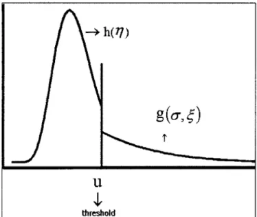
The proposed model assumes that observations under the threshold, u, come from a certain distribution with parameters "1, denoted here H(.lry), while those above the threshold come from a GPD, as introduced in equation (1). Therefore, the distribution function F, of any observation X, can be written as

{ H(xlry)

F(xlry,

ç,

a, u)

=

H(ulry)

+

[1 -

H(ulry)]

G(xlç,

a, u) ,x _{, x}

<

_"2

u _u

(2)

For a sample ofsize n, x = (Xl, ... ,xn ) from F, parameter vector 8 = ("1, a,

ç,

u),

A

=

{i :

Xi

<

u} and B

=

{i :

Xi

"2

u}, the like1ihood function is,

L(8;x)

=II

h (xlry)

II

(I-H(ulry))

Ｈｾ｛Ｑ＠

+

Ç(Xi -U)]

_(lt

O

) (3)

A B a a +

for

ç

i-

O, and L(8;

x)

=TIA h (xlry)TIB (1 - H (ulry)) Ｈｾ･ｸｰ＠ {(Xi - u)

la}),

for

ç

=

O.

Figure ! represents, schematically, the mode!. As it can be seen, the thresho!d

u is the point where the density has a discontinuity. Depending on the parameters the density jump can be larger or smaller, and in each case the choice ofwhich observations will be considered as exceedances can be more obvious or less evident. The smaller the jump the more difficult can be the estimation of the threshold. Fitting a nonparametric model to the data below the threshold allows smooth changes in the distribution around

u. Strong discontinuities, or large jumps, indicate separation ofthe data. Consequent1y, it is expected that the parameter estimation wou!d be easier. On the other hand, density functions that are relatively smooth might represent an interesting challenge to our modeling structure. The parameters in our simulations were chosen in order to produce both situations.

Figure! about here

As stated before, one goal ofthis work is to analyze ifthe choice ofthe distribution for observations below the threshold may infiuence, and how, the threshold estimation. In addition, we are interested in analyzing whether the proposed mode1 exhibits good data fitting when compared to other analyses presented in the literature.

Finally, it is worth mentioning that our mixture mode! can be extended to, for ins-tance, a mixture of distributions below the threshold. In the next section we combine (3)

(6)

I

with a prior distribution for the parameters in order to enable one to perform posterior inference.

3 Prior Elicitation and Posterior Inference

Recalling, the parameters in the modeI are (J

=

("1, u,

ç,

a). The prior distribution is now described.

3.1 Prior for Parameters above Threshold

In extreme value analysis data are usually sparse, then information from experts can be use fui to supplement the information from the data. It is reasonable to hope that experts should provi de relevant prior information about extremai behavior, since they have specific knowledge of the characteristics of the data under study. Nonetheless, expressing prior beIiefs directly in terms of GPD parameters is not an easy task. The idea we use here is due to Coles and Tawn (1996a), Coles and Powell (1996) and Coles and Tawn (1996) and refers to the elicitation of information within a parameterization on which experts are familiar. More precisely, by the inversion of equation (1), we obtain the 1 - p quantile ofthe distribution,

(4)

where q can be viewed as the return levei associated with a return period of l/p time units. The elicitation of the prior information is done in terms of (ql, q2, q3), in the case of location-scale parameterization of the GPD, for specific values of PI

>

P2

>

P3.

Therefore, parameters are ordered and ql

<

q2

<

q3. So, Coles and Tawn suggest to work with the difTerences di

=

qi - qi-l, i

=

1,2,3 with qo

=

el, where el is the physical lower bound of the variable. They suggest setting di ｾ＠ Ga( ai, bi ) for i

=

1,2,3. The case of el

=

O is used in most applications. Independent prior distributions are assumed for the difTerences di 's. The prior information is elicited by asking the experts the median and 90% quantile (or any other) estimates for specific values of P

that they are comfortable with. U sually, 10, 100 and 1 000 time periods are considered, which correspond, respectively, to PI

=

0.1, P2

=

0.01 and P3 = 0.001. After that, the elicited parameters are transformed to obtain the equivalent gamma parameters. For i

>

1, neither di nor qi depend on u. For i

=

1, p(d1Iu) was approximated by

(d1Iu*) ｾ＠ Ga( ai (u'),

bd

u*)) where u* is the prior mean for u.

In the model proposed here, we are not considering the GPD's location parameter, so only two quantiles are needed in order to specify the GPD parameters, a and

ç.

Therefore, we have the following gamma distributions with known hyperparameters:

dI = ql ｾ＠ Ga(al' bl ) and d2 = q2 - ql rv Ga(a2' b2) The marginal prior distribution

(7)

7r(a,ç) ex

｛ｕＫｾＨｐｉￇＭＱＩｲｬＭＱ･ｘｐ｛Ｍ｢ＱｻｕＫｾＨｐｬￇＭＱＩｽ｝＠

x

｛ｾＨｐＲￇ＠

-

PI

Ç)]

a2-1

exp

｛Ｍｾ＠

{

ｾ＠

(P2Ç

-

PI

Ç) } ]

x

1-

f

[(P1P2)-Ç(lOgP2

-logP1) -

P2

Ç

logP2

+

Plç IOgP1]

1

(5) where

a1, b1, a2

and

b2

are hyperparameters obtained from the experts information, for example in the form ofthe median and some percentile, corresponding to return periods Ofl/P1 and 1/P2. The prior for q1 should in principIe depend on u. This would impose unnecessary complications in the prior formo In this paper, this dependence is replaced

by dependence on the prior mean of U.

Some authors find that it is interesting to consider the situation where

ç

=

O. In

this case, we can set a positive probability to this point. The prior distribution would consider a probability q if

ç

=

O and 1 - q if

ç

-I

O, spreading the elicited prior shown above to this last case. From the computational point of view this model would not lead to any particular complications.

3.2 Prior for the Threshold

There are many ways to set up a prior distribution for U. We can assume that u follows

a truncated normal distribution with parameters (J.lu, ｡ｾＩＬ＠ truncated from below at

e1

with density,

( I 2 ) _ _ 1_ exp{ -O.5(u - J.lu)2 Ｏ｡ｾｽ＠

7ruJ.lu,au,e1 - _yｾ＠_{ＲＷｲ｡ｾ＠}

fl,.[ (

_{'*' -}

_e1

_-

_{J.lu a u}

)/ 1

(6)

with J.lu set at some high data percentile and ｡ｾ＠ large enough to represent a fairly noninformative prior.

This prior is used in the simulation study and the details are shown in the next section. A continuous uniform prior is another alternative. A discrete distribution can also be assumed. In this case, u could take any value between certain high data

percentiles, that can be called hyperthresholds, as used in the application in section 5. Since the number of observations is usually high in applications, when the discrete prior is based on the observations the choice between discrete or continuous prior is immaterial for practical purposes.

One approach to the discrete prior for u is presented by Bermudez, Turkman and Turkman (200 I). They suggest threshold estimation by setting a prior distribution for the number of upper order statistics. In this case, the threshold is indirectly chosen and

given by the data percentile corresponding to the number of exceedances. We could also have assumed one more leveI to set the prior distribution for u, this would require setting a prior distribution for the hyperthresholds.

3.3 Prior for Parameters below the Threshold

(8)

h(xl17). It is always better try to obtain a conjugate prior to simplify the problem analytically. In a general way we assume 17 rvp with density 7r.

Ifthe distribution h(xl17) chosen is a Gamma, we have 17

=

(o, (3), o as the shape and {3 as scale parameter. But, instead of working with o and {3, parameters of the Gamma distribution, we reparameterize and think, in terms ofprior specification, about o and J-L

=

oi (3. J-L has a more natural interpretation; it is the prior expected value

for the observational mean below threshold. Also, it is more natural to assume prior independence between the shape parameter and the mean. We then set, o rv Ga( a. b)

and J-L rv Ga( c, d), where a, b, c and dare known hyperparameters. The joint prior of

7]

=

(o, (3) will then be,

(7)

3.4 Posterior Inference

From the likelihood (3) and the prior distributions specified above, we can use Bayes theorem to obtain the posterior distribution, which has the following, taking a Gamma distribution for data below the threshold, functional form, on the logarithm scale

n

logp(Olx)

=

K

+

L

I(xi

<

u) [o log,B - logf(o)

+

(o - 1) logxi - {3x;]

i=1

n

[r

(30 ] n

ＫｾｉＨｸｩＲｵＩｬｯｧ＠

l-lo

f(0)tO

- 1e-3tdt

ＭｾｉＨｸｩＲｵＩｬｯｧ｡＠

ｬＫ￧ｾ＠

[Ç(Xi-U)]

ＭＭＭｾｉＨｸｩ＠ 2u)log 1+ a

ç

i=1

o o o

+(a - 1) log 0 -bo

+

(c - 1) log(

'8) -

d(

'8)

+

log( 72)

,

,B

1

(u

-

J-Lu ) 2 {

a

_ç }

- 2

ｾ＠

-

b1 U

+

ｾ＠ (Pl - 1)

+(a2 - 1) log

[u

+

ｾ＠

(p;ç - p;-ç) ] - b2

{U

+

ｾＨｰ［ￇ＠

- P;-Ç)}

+

log

1-

f

[(P1P2) -Ç (log P2 - log Pl) - p;ç log P2

+

p;-ç log Pl ]

1

(8)

where K is the normalizing constant. It is clear that this posterior distribution has no known closed form distribution making analytical posterior inference infeasible. Note that the posterior written out above is shown with a normal prior for the threshold and with the likelihood for the case where

ç

=I-

O. However, the case where

ç

=

O is also considered in the algorithm used in the applications.

(9)

either sample (j at once, or break it into smaller blocks to be drawn from. It will de-pend on the convergence rate in each case. Because of the features of the model, we are drawing the shape parameter

ç

of the GPD first, since the scale parameter (J and

the threshold depend on its signo If

ç

is negative, (J and u have restrictions as one can

see in the definition of GPD distribution (1). Following

ç,

(J and u are drawn

indivi-dually and in this order. Lastly, "l is jointly drawn. In the case of gamma parameters,

"l = (o, (3). The use of Metropolis-Hastings algorithms requires the specification of candidate distributions for the parameters.

4 A

Simulation Study

We entertained a wide range of scenarios, focusing on generating skewed and heavy-tailed distributions. For the sake of space, only a small but revealing fraction of them is presented here, with further details directed to Behrens, Lopes and Gamerman (2002) (BLG, hereafter). The parameters used for the simulations presented here are p

=

0.1, o

=

(0.5,1,10),

ç

=

(-0.1, -0.45,0.2), and n

=

(1000,10000). AIso, the scale parameters ;3 and (J were kept fixed (1/;3 = (J = 5), since their changes do not

inftuence the estimation. The sample size n and p automatically define the value of u.

We chose

ç

=

-0.45 for generating lighter tails and for avoiding unstable maximum likelihood estimation, while

ç

=

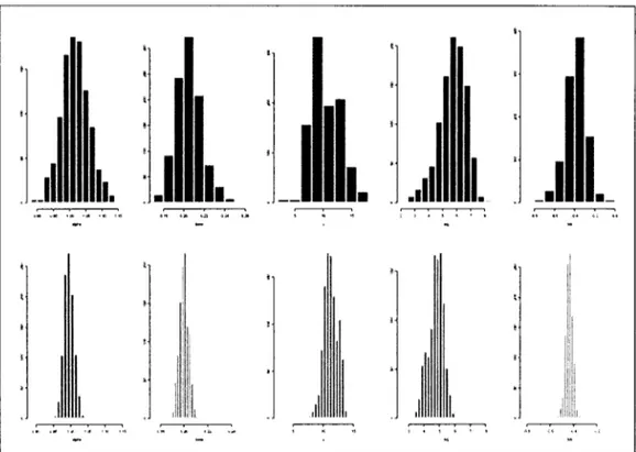
0.2 generates heavier tails. Table 1 summarizes our findings based on the 18 data sets while Figure 2 shows the histograms ofthe marginal distributions of the model parameters when o

=

1.0 and

ç

=

-0.45. As one would expect, for ali entertained datasets, the 95% credible posterior intervals contain the true values. Similar results were found when p

=

0.01 and p

=

0.001 (see BLG).

Table 1 and Figure 2 about here

It is important to verify if observations from other distributions, different from Gamma, are well fitted by our model. Some variations using Weibull data for the center of the distribution were considered and GPD results were not affected. Despite the similarities between the distributions, these results tentative\y point to robustness ofthe models proposed here.

5 Modelling the N asdaq 1 00 Index

The next step will be the application of the model to real data and to analyze how the methodology performs in different situations in different fields. We now apply our approach to Nasdaq 100, an index of financiai market, from January 1985 to May 2002 (N= 4394). The dataset was chosen given its importance to financiai market and the presence of many extreme events and it was taken from Yahoo financiai site -http://finance.yahoo.comlq?d=t&s=''IXIC. The original data, daily c\ose index, is con-verted to daily increments in the following way:

Yt

=

100

IPt! P

t - 1 - 11

(10)

negative large returns are important in most practical volatility evaluations by risk an-alysts. The usual treatment involves removal of these temporal dependences through time-varying volatility formulations. Our interest here, however, is to concentrate on large values ofreturns and therefore we did not perform any such standardization to the data. Figure 3 displays a histogram of the data. As we can see, there is indication of heavy tailed data. Our main goal is to compare the results obtained by our mode! with those obtained using a maximum like!ihood (ML) approach. Also, we want to test the efficiency of our method in the extrapolation issue. The model used in this application uses a Gamma distribution to fit the data be!ow the threshold.

Figure 3 about here

A descriptive analysis is presented below in order to get more fee!ing about the data behavior. For the ease of notation let N be the sample size,

[xl

is the integer part of the number x and Y(i) the ith order statistic of data (YI, ... , YN), such that Y([pN]) is the

lOOp data percentile, e.g. Y([O.70N]) is the 70% data percentile.

Table 2 shows the ML estimator for (J" and

ç

considering different values of u. There

are no important changes in the estimates of (J" and

ç

as the value of U is changed.

We cannot observe any pattern in the

ç

estimates with changes with the number of exceedances considered. When the number of exceedances is around 2% of the data, the estimates of (J" and

ç

become very unstable. We have also ca1culated the conditional

Bayes estimators for the extreme parameters considering the same values of u used to obtain the ML estimators. As we can expect, a small increase in the posterior mean of

(J" is observed since the greater value of u implies less exceedances or less data points

to estimate (J" (its variance increases with u). The results are in Table 2 and we can

see that the estimate of

ç

are consistent if compared with its Bayesian estimate. For the other values we observe an increase in the posterior mean for the scale parameter, since we have more uncertainty incorporated in the mode!. Also the credibility intervals are larger for both extreme parameters.

Table 2 about here

A bivariate analysis of (J" and

ç

is also performed based on the likelihood and

pos-terior distributions to analyze correlation between blocks of parameters. We have taken the conditional distributions considering different values of u, Y([O.5N]), Y([o. 7N]).

Y([O.9Nj) Y([O.95Nj),and the ML estimators for (J" and

ç

and the moment estimators for

Q and {3. Conditional on u the vector (Q, {3) is independent of ((J", Ç). The values of Q

and ,8 that maximize the likelihood function are not much affected by changes in the threshold. Only the scale parameter, {3, presents a small variation since the number of observations used to estimate it changes with u. The same happens when we look at the conditional likelihood of (J" and

ç.

Similarly, the values of (J" and

ç

that maximize

the conditionallikelihood are dose to the ML estimators shown in Table 2.

Flat priors were considered for Q, {3, (J" and

ç,

and hyperparameters were ca1culated

as described in section 3. The chosen values were aI

=

0.1, bl

=

aJ/19.8, a2

=

0.9

and ｾ＠ = a2/29.8. A uniform discrete prior was assumed for the threshold u and the values ofthe hyperparameters are described in the appendix.

Conditional on u, (J" and

ç,

the values of Q and ,8 that maximize the posterior are

(11)

to those shown in the likelihood analysis. A slight difference can be noticed when the threshold chosen is Y([O.5Nj).

Based on the the graphs in Figure 3, the initial values to start the chains were chosen and this is described in the Appendix. The posterior mean of Q and

13,

1.0202 and

1.2816 respectively, are very c\ose to the moment estimators. The posterior mean and variance of a and

ç

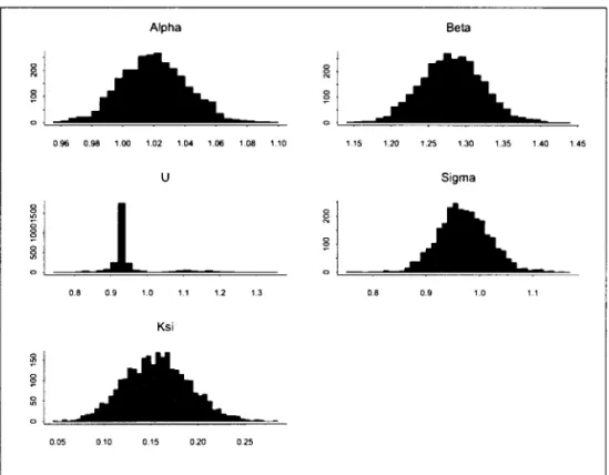
are shown in Table 2. As we said above, we have chosen two similar discrete prior distributions to perform the analysis, and since we also got similar results with both cases only the second one is shown in Table 2.

Convergence was achieved after few iterations and Figure 4 presents the histograms of the distributions of each parameter. The parameter

ç

has a distribution centered in the ML estimator and Q and

13

centered in the moment estimators. The Bayesian approach

shows a larger estimate for a than the c\assical one, while the credibility interval of

ç

inc\udes its maximum likelihood estimate. The distribution ofthe threshold, u, seems to be bimodal, one ofmodes being highly concentrated around Y([O.58Nj) and the second mode concentrated around Y([O.9027Nj), so the posterior mean is Y([O.7586Nj). The first

mode has probability 0.67 around it and the second mode has probability 0.10 around it.

Figure 4 about here

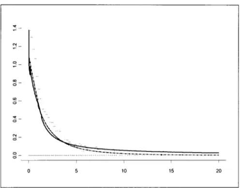
In order to observe how the model fits the data and to analyze the behavior of the model for future observations, we computed the predictive distribution. Figure 3 shows the predictive distributions superimposing the histogram of the data. The solid line is the Bayesian predictive distribution, p (Yldata)

=

J

p (Yle) p (eldata) de, and the dashed line is an approximate Bayesian approach, p (yldata)

ｾ＠

p (YIB) where

B

=

E Ｈ･ｬ､｡ｾ｡ＩＬ＠ which corresponds to concentrating alI the information in the

pos-terior mean,

e,

a reasoning similar to that used for c\assical prediction. We can see that the difference between the two approaches is not so significant in the center of the distribution, while the Bayesian approach gives higher probabilities in the tail. The ap-proximate Bayesian predictive distribution underestimates the probabilities for events considered extremes.

Table 3 about here

In general terms, the results show that the estimated extreme quantiles obtained from the (fulIy) Bayesian predictive distribution se em to be more conservative than the ones produced by using plug-in estimation such as the approximate Bayesian or the c\assical approaches. For instance, in Table 3 we can see that P (X

>

5.35)

=

0.01, which means that an extreme event higher than 5.35, occurs, on the average, once in 5 months using the approximate Bayesian approach, since our data are taken daily. If we look at the fulIy Bayesian estimates, we have P (X

>

5.35)

=

0.04, which means that an extreme event higher than 5.35 only takes 1.25 months to occur on the average. In a decision making setting, the fulIy Bayesian approach represents one's risk averse behavior. This is caused by the incorporation of the uncertainty about the parameters of the model. This aspect of the Bayesian approach has already been noted by other authors. Coles and Pericchi (2003) showed that this leads to more sensible solutions to real extremes data problems than plug-in estimation.

(12)

"

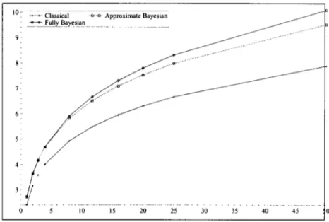
Figure 5 shows the retum leveis associated with retum periods from I week to I year. The shorter retum periods in the Bayesian approach, associated with any given retum levei, are a direct consequence ofthe thicker tail observed in Figure 3. Again, we can see that the fully Bayesian approach is more conservative than the c\assical and approximate Bayesian approaches. An extreme retum levei in the fully Bayesian approach takes less time to occur on average than the same retum levei considering the other two approaches.

Figure 5 about here

6 Conclusions

In this paper we suggest an altemative to the usual analysis of extreme events. Infe-rence is based on a mixture model with gamma distribution for observations below a threshold, and a GPD for observations above it. Ali observations are used to estimate the parameters present in the model, inc\uding the threshold.

Different approaches have been tried in the Iiterature, but in none of them is the threshold treated as a parameter in the estimation processo The available methods choose the threshold empirically, even those using Bayesian methodology.

A simulation study was performed and the results have shown that we obtained good estimates of the parameters. In spite of this fact, the threshold was at times hard to estimate, especially when the sample size was not large enough. In general, the gamma parameters converged very fast, while the GPD parameters, a and

ç,

and u

needed more iterations. These last three parameters sometimes demonstrated a strong correlation between their chains, but this did not affect the convergence.

This wide range of scenarios allowed us to analyze the behavior of posterior den-sities under different situations. It seems that the shape of the distribution is not a problem in parameter estimation. For sufficiently large samples, parameter estimates were very c\ose to the true value even for data which was strongly skewed andJor did not have a smooth density function. The problems with convergence, and consequently with parameter estimation, arise when the number of observations is smal\. The pro-posed model here, although simple, is able to fit different situations. Results obtained applying our Gamma-GPD model to data simulated from other distributions showed a good performance.

Classical methods for analyzing extreme events require a good choice of the thre-shold to work well. Our proposed method avoids this problem while considering the threshold as a parameter ofthe model and allows prior information to be incorporated into the analysis.

(13)

dis-tributions, where the fully Bayesian inference seems to fit better to more extreme data than the approximate Bayesian approach.

It is also interesting to look at the retum leveI associated with a retum period of

l/p units oftime. We show the plot ofthese values for a range ofretum period from I week to 1 year and results has shown that the fully Bayesian approach is, again, more conservative, than the cIassical and approximate Bayesian approaches. This means that a certain retum leveI is associated with a shorter retum period in the fully Bayesian approach.

A similar methodology considering other parametric and nonparametric forms for the distribution of the observations below the threshold can also be considered. Tan-credi, Anderson and O'Hagan (2002) tackles the threshold problem in a similar but independent way. They model the non extreme data (below threshold) by a mixture of uniforms. The use of other parametric forms, Iike Student-t distribution, will allow the estimation of both tails, as needed in many financiaI and insurance data, where interest Iies in the estimation not only on the large cIaims (or gains) but mainly on large losses. Also, a more exhaustive study about other distributions below the threshold should be performed.

References

Behrens C, Lopes HF, Gamerman, D (2002) Bayesian analysis of extreme events with threshold estimation. Technical Report, Laboratorio de Estatistica, Universi-dade Federal do Rio de Janeiro.

Beirlant J, Vynckier P, TeugeIs, JL (1996) Excess functions and estimation of the extreme-value indexo Bernoulli, 2, 293-318.

Bermudez PZ, Turkman MAA, Turkman KF (2001) A predictive approach to tail probability estimation. Extremes, 4, 295-314.

Coles SG, Pericchi LR (2003) Anticipating catastrophes through extreme value modelling. Applied Statistics, 52,405-16.

Coles SG and Powell EA (1996) Bayesian methods in extreme value modelling: a review and new developments. International Statistical Review, 64, pp. 119-36. Coles SG, Tawn JA (1991) Modelling extreme multivariate events. Journal 01 the Royal Statistical Society B, 53, 377-92.

Coles SG, Tawn JA (1994) Statistical methods for multivariate extremes: An ap-plication to structural designo Applied Statistics, 43, 1-48.

Coles SG, Tawn JA (1996) A Bayesian analysis of extreme rainfall data. Applied Statistics, 45, 463-78.

(14)

Jour-nal ofthe Royal Statistical Society B, 52, 393-442 (With discussion.)

Doornik JA (1996) Ox: Object Oriented Matrix Programming, 3.1 Console Ver-sion. Nuffield College, Oxford University, London.

DuMouchel WH (1983) Estimating the stable index Q in order to measure tail

thickness: a critique. The Annals of Statistics, 11, 10 19-31.

Embrechts P, Klüppelberg C, Mikosch T (1997) Modelling Extremai Events for Insurance and Finance. Springer: New York.

Embrechts P, Resnick SI, Samorodnitsky G (2001) Extreme value theory as a risk management tool. XXVIII International ASTIN Colloquillm. Cairns, Australia. Frigessi A, Haug O, Rue H (2002) A dynamic mixture model for unsupervised tail estimation without threshold selection. Extremes, 5,219-235.

Gamerman D (1997) Markov Chain Monte Carlo: Stochastic Simlllationfor Bayesian inference. Chapman & Hall: London.

GeIman A, Rubin DB (1992) Inference from iterative simulation using multiple sequences. Statistical Science, 7,457-511.

Geweke J (1992). Evaluating the accuracy of sampling-based approaches to cal-culating posterior moments. In Bayesian Statistics 4, (ed. Bernardo 1M, Berger

10, Dawid AP, Smith AFM). Clarendon Press, Oxford, UK.

Heidelberger P, WeIch P (1983). Simulation run length control in the presence of an initial transient. Operations Research, 31, 1109-44.

Mendes B, Lopes HF (2004) Data driven estimates for mixtures. Computational Statistics and Data Analysis (accepted for publication)

Pickands J (1975) Statistical inference using extreme order statistics. Annals of Statistics, 3, 119-131.

Robert CP, Casella G (1999) Monte Carlo Statistical Methods. Springer: New York.

Smith BJ (2003) Bayesian Output Analysis Program (BOA) Version 1.0. College of Public Health, University of Iowa, US.

Smith RS (2000) Measuring risk with extreme va\ue theory. In Embrechts P ed.

Extremes and lntegrated Risk Management. London: Risk Book, 19-35.

(15)

7 Appendix

In this appendix we describe the Markov Chain Monte Carlo algorithm used to make approximate posterior inference and also the implementation details. Gamerman (1997) and Robert and Casella (1999) are comprehensive references on this subject. We have used the Ox language when developing the MCMC algorithms (see Doornik, 1986). It

took us about 2 hours, on average, to run 10000 iterations using a Pentium III PC with 833MHz.

7.1 Algorithm

Simulations are done via Metropolis-Hastings steps within blockwise MCMC algo-rithm. So, candidate distributions for the parameters evolution must be specified. The candidate distributions used in the algorithm are presented below as well as the steps of the algorithm. Suppose that at iteration j, the chain is positioned at O(j)

=

(oh), j3U),

uU), a(j),çU»). Then, at iteration j

+

1 the algorithm cycles through the following steps:

7.1.1 Sampling

ç

Ç* is sampled from a N(ç(j) , Vç)I(-aU)/(M - u(j»),oo) distribution, where Vç is an approximation based on the curvature at the conditional posterior mode, and M

=

max(xl, ... , Xn). Therefore, ç(j+l)

=

Ç* with probability nÇ where

{

(ç(J)+al))

!(M-UiJ )) }

. p(O*lx)

yV;

nÇ

=

mm 1, --_ -

---'-,---'---,''-p(Olx) ＨￇＪＫ｡ＨＩｾＭｕｉＩＩＩＩ＠

for 0* = (n U),j3(j), u(j), a(j),Ç*),

e

= o(j) and <1>(.) is the standard normal's

cumu-lative distribution function. 7.1.2 Sampling a

If ç(j+l) ::::: O, a* is sampled from a Ga(aj,bj ) distribution, where aj/bj

=

a(j)

and aj/b;

=

_Va.Ifç(j+l)

<

O, a* is sampled from a N(a(j),

Va)I(_çU+l)(Af-u (j»), 00) distribution, where Va is an approximation for the concavity in the

condi-tional posterior mode. Therefore, a(j+l) = a* with probability na where

_ . { p(O*lx) g(a(j)laj,bj )}

na - mm 1. _p(Olx)-

(I

b) ,

9 a* a*, *

(16)

7.1.3 Sampling u

The threshold parameter u* is sampled from a N(u(j), V_u)I(a(j+1), M) distribution with a(j+l)

=

min(xI,' .. ,x_{n ),}if ç(j+l)

2:

0, and a(j+l)

=

M

+

(T(j+l) /ç(J+I), if

çU+I)

<

O. Again, Vu is a value for the variance which is tuned to allow appropriate

chain movements. Therefore, u(j+l)

=

u* with probability Ou where

{

*

(M-U(j») _

(aIJ+1)_u(j»)}

_ . 1 p((} Ix) ｾ＠ｾ＠

Ou - mln ,

-p((}lx)

(Af-

7U*) _

(aIJ+1)-u*)

ｾ＠ｾ＠

for 0*

=

(o(j), (3(j), u*, (T(j+1) , ç(j+l») and

B

=

(o(j), (3(j), u(j) p(j+1) , ç(j+l»).

In the case where u has a discrete prior we have to follow the same mo dei restric-tions as before. Then, the candidate distribution is: If ç(j+l)

2:

0, u* ｾ＠ Ud (ql. q2),

a discrete uniform distribution on data quantiles from ql to q2, where q2 can be any high quantile as, for instance, M, while ql can be any quantile, as long as ql

<

q2.

It is important to keep in mind that ql must be small enough to reduce model bias and large enough to respect the asymptotic properties of the model. Analogously, if

ç(j+l)

<

0, u* ｾ＠ Ud(ql,q2), with ql

2:

M

+

(T(j+1)/ç(j+I). In the discrete case,

Ou = min{p((}*lx)/p(Blx)}.

7.1.4 Sampling

°

and .8

0* and (3* are sampled, respectively, from a logN(o(j),

Vc,)

and a GI(aj,bj ) dis-tributions, with aj/bj

=

(3(j), aj/bJ

=

VB. V" and V3 are approximations for lhe curvatures at the conditional posterior modes. Therefore, (O(j+l), a(j+l») = (Q*. 8*) with probability

for 0*

=

(0*,(3*, U(j+l), (T(j+l),ç(j+l»),

B

=

(oU).j3(j), uU+I)p(j+I),ç(j+I»),

a* /b*

=

(3*, a* /b*2

=

V3, h(

'Ic,

d) is the log-normal density with mean

c

and variance

d, and g(·lc. d) is lhe gamma density with parameters c and d.

7.2 Implementation

Our implementation involved running a few parallel chains starting from ditTerent re-gions ofthe parameler space. The first few draws from the chains were used for tuning

(17)

8 Figures and Tables

u

ｾ＠

threshold

Figure 1: Schematic representation ofthe mode)

(18)

J

I.

Figure 2: Marginal posterior histograms of modeI parameters based on data generated from p = 0.1. Q = 1, (3 = 0.2, a

=

5 and

ç

= -0.45. Top row, n=1000 (u = 11.85).

(19)

co

Ó

<D

o

..,.

o

N

Ó-o

o

o 5 10 15 20

(20)

Alpha Beta

ｾ＠ｾ＠

ê o _o

096 0.98 100 1.02 1.04 1.06 1.08 1.10 115 1.20 1.25 1.30 1.35 1.40 145

U Sigma

ｾ＠ I

1

ｾ＠

_ê

ｾ＠

o ,

0.8 09 1.0 1.1 1.2 1.3 0.8 0.9 1.0 1.1

Ksi

ｾ＠

ê o

ｾ＠

0.05 0.10 0.15 020 025

(21)

•

10 ｾ＠ｾＨｩｬＧ［ｾ｣ＭＮｉＭＭＮｾＭＮｯＭＮ＠ Ac-pp-ro---Cxi-m.-te-:CB.-ye---Csi-.n

. ｾ＠ｆｾＡＡｌｾＩＧｾｳｩｾ｟ｾ＠

9-

8-

6-5·

'I

3{

ｾ＠ . --ｾ＠ＭｾＭｾ＠Ｎ｟ＭｾＭＭＭＭＭ｟Ｎ＠

10 15 20 25 30 35 40 45

Figure 5: Retum leveI associated with retum period from I week to 1 year. The parameter values used to calculate the retum leveI in the cIassical approach refer to those where u

=

0.93

=

Y([o. 7 N]).

20

(22)

• ...,

•

(23)

• ..,

·

•

p u a

ç

Classical 0.5 0.57 0.6305 0.2396 0.7 0.93 0.8176 0.1466 0.9 2.11 0.7435 0.1689 0.95 2.92 0.7171 0.1786 Bayesian 0.5 0.57 0.7480 0.2404 conditional on u [0.07;0.80] [0.18;0.30]

0.7 0.93 0.9579 0.1609 [0.87; 1.04] [0.09;0.23] 0.9 2.11 1.0827 0.1945

[0.92; 1.24] [0.08;0.32] 0.95 2.92 1.1869 0.2297

[0.02; 1.46] [0.03;0.42] Bayesian

-

0.9619 0.9735 0.1567

[0.79; 1.13] [0.86; 1.08] [0.09;0.23] Table 2: Summary of extreme parameter estImators: posterior means and 95% credibility intervals, between brackets, ofu, a and

ç;

ML estimators

for a and

ç

for different values of u

=

Y«(PNJ).

(24)

• _..

-•

N.Cham. P/EPGE SA L864b

Autor: Lopes, Hedibert Freitas

Título: Bayesian analysis of extreme events with thresholJ

(25)

• '1

1

..

Quantiles Empirical FB AB 2.11 0.9 0.86 0.897 2.92 0.95 0.91 0.947 5.35 0.99 0.96 0.99 9.00 0.999 0.98 0.998 Table 3: Extreme tail probability using the empirical data distribution, (fully) Bayesian (FB) predictive distribution

and approximate Bayesian (AB) predictive distribution.

FUNDAÇÃO GETULIO VARGAS

BIBLIOTECA

ESTE VOLUME DEVE SER DEVOLVIDO A BIBLIOTECA NA ÚLTIMA DATA MARCADA

1l0UT

?lhO

23

BIBLIOTECA