SOIL WATER CONTENT TEMPORAL-SPATIAL
VARIABILITY OF THE SURFACE LAYER OF A LOESS
PLATEAU HILLSIDE IN CHINA
Wei Hu1,2,3; Ming An Shao2*; Quan Jiu Wang2; Klaus Reichardt4
1
Key Laboratory of Water Cycle and Related Surface Processes, Institute of Geographical Sciences and Natural resources Research, Chinese Academy of Sciences, Beijing 100101, China.
2
State Key Laboratory of Soil Erosion and Dryland Farming on the Loess Plateau, Institute of Soil and Water Conservation, Chinese Academy of Sciences & Ministry of Water Resource, Northwest A &F University, Yangling 712100 Shaanxi, China.
3
Graduate School of the Chinese Academy of Sciences, Beijing 100039, China. 4
USP/CENA - Lab. de Física do Solo, C.P. 96 - 13418-900, Piracicaba, SP- Brasil. *Corresponding author <[email protected]>
ABSTRACT: Surface soil moisture exhibits an important variability in terms of spatial and temporal domains, which may result in critical uncertainties for agricultural water management. The purposes of this study were (i) to characterize the temporal dynamics and stability of the spatial variability of the surface 0-6 cm soil water content θ on a hill-slope; (ii) to investigate issues related to soil moisture conditions including dominating factors on soil moisture and to the estimation of the mean θ. During a period of more than one month θ was measured on thirteen days by Frequency Domain Reflectometry using a 10 × 10 m grid of measurement points covering a 60 × 280 m domain within a hill-slope of the Loess Plateau in China. Soil water content exhibited a moderate variability for each measurement date, and the correlation length (λ) for θ ranged from 8.4 to 27.7 m. With the soil becoming drier, λ decreased, the CV% and the sampling number for accurate mean θ estimation increased. Aspect, elevation, organic matter content, clay content, and bulk density were the main influencing factors, whose extent of influence weakened with decreasing θ. Based on time stability analysis and on the correlation of mean relative difference of θ with the relative difference of dominating factors, mean θ values were well estimated, with a better accuracy under wetter conditions.
Key words: surface soil moisture, coefficient of variation, correlation length, temporal stability
VARIABILIDADE TEMPORAL E ESPACIAL DA UMIDADE DO SOLO
NA CAMADA SUPERFICIAL DE UMA ENCOSTA DO “LOESS
PLATEAU” NA CHINA
RESUMO: A umidade da camada superficial do solo apresenta uma variabilidade importante nos domínios espacial e temporal, que pode levar a incertezas críticas para o manejo agrícola da água. Os objetivos deste estudo incluíram: (i) a caracterização da dinâmica temporal e da estabilidade da variabilidade espacial da umidade θda camada 0-6 cm em uma encosta em declive; (ii) investigação de parâmetros ligados às condições de umidade, incluindo fatores dominantes da umidade na estimativa de um valor médio de θ. Durante um período de mais de um mês, θfoi medida em 13 dias com auxílio da técnica da Refletometria do Domínio da Frequência, em uma grade de 10 × 10 cm, cobrindo uma área de 60 × 280 m, situada em uma encosta do “Loess Plateau” da China. A umidade do solo apresentou variabilidade moderada em cada data de medida e o alcance da correlação (λ) para θvariou de 8,4 a 27,7 m. Com o solo mais seco, λ decresceu, o CV% e o número de amostras
necessário para obter uma média precisa, aumentaram. O aspecto, a elevação, o conteúdo de matéria orgânica e a densidade do solo foram os principais fatores interferentes na umidade, cuja intensidade de influência diminuiu com a umidade. Baseado na análise de estabilidade temporal e na correlação da diferença relativa média de θ com a diferença relativa média dos fatores dominantes, valores médios de θ puderam ser mais bem estimados, com maior precisão sobre condições mais úmidas.
INTRODUCTION
Shallow surface soil moisture is a key status variable in hydrologic processes on the land surface, which tends to be variable in both time and space. Therefore, the knowledge of the characteristics of soil moisture variability is important for understanding and predicting many hydrologic processes (Western et al., 2004). Variability of soil moisture has been studied ex-tensively in the past half century using either classical statistics (Hawley et al., 1982), geo-statistics (West-ern et al., 2002), or time series analysis (Timm et al., 2006). Relatively less emphasis has however been given to the temporal domain as compared to the spa-tial scale.
Top layer soil moisture variability can be con-trolled by a large number of factors, such as soil prop-erties (Hawley et al., 1983), topography (Western & Blöschl, 1999), and vegetation (Reynolds, 1970). It is not straightforward to recognize the different domi-nating processes or factors influencing soil moisture distributions along different study areas since the domi-nating factors may also be different under different soil moisture conditions (Grayson et al., 1997; Famiglietti et al., 1998; Leij et al., 2004).
Since the contribution of Vachaud et al. (1985), there has been an increasing interest in temporal sta-bility of soil moisture (Grayson & Western, 1998; Starks et al., 2006). Based on the time stability analy-sis, Grayson & Western (1998) pointed out that if there are definable features of the terrain and of the soils that could be used to define locations a priori, then the mean soil moisture could also be well deter-mined only from these selected points.
The purpose of present study was, therefore, to investigate the temporal and spatial variability of the soil water content of the 6 cm top layer on a hillslope of the Loess Plateau. Specific objectives were (i) to characterize the temporal dynamics of the magnitude and pattern of the soil moisture variability; (ii) to un-derstand the relative roles of soil and topographic fea-tures under different soil moisture conditions; (iii) to obtain the number of samplings needed for the esti-mation of the mean soil moisture within a chosen sig-nificance level based on classical statistics; and (iv) to estimate the mean soil moisture based on time stabil-ity analysis and the relationship of soil moisture with its dominating factors.
MATERIAL AND METHODS
Field site description
The study was carried out at the Beigeba hillslope of the Liudaogou watershed located in the
Shenmu County, Shaanxi Province, China (110º21' to 110º23' E and 38º46' to 38º51' N) (Figure 1), with a maximum elevation of 1,256 m above sea level. The average slope is 19° with a total slope length of 280 m. The soil (cultivated loessial soil), is an Ust-Sandic Entisol of sandy loam texture, and is mainly covered by Purple medic (Medicago sativa L.) and scattered shrub (Caragana korshinskii). The area is character-ized by steep gullies and hills, and the soil is loess-de-rived and easily eroded (Tang et al., 1993). Mean an-nual precipitation is 437 mm, nearly half of which is received from June to September. The potential evapo-transpiration is 785 mm, with a mean aridity index of 1.8 and annual temperature of 8.4ºC, belonging to mod-erate - tempmod-erate and semi-arid zones.
Sampling and measurement
A total of 203 sampling points were setup ev-ery 10 m along two perpendicular directions (Figure 1). Since 26 points were located deep in the gullies, 177 remained available for measurements. At each sam-pling point the Frequency Domain Reflectometry (FDR) technique was used to determine the volumet-ric soil water content (θ, cm3 cm-3
) of the top soil layer (0-6 cm). On 13 days, from May 17 to July 21, 2005, θ was measured along the 280 m of the toposequence slope. In order to reduce the possible uncertainties caused by the timing of samplings, the measurements started about 90 minutes before darkness everyday, and each measurement finished within 70 minutes. Further-more, measurements with the FDR probe of 6 cm length were taken within a soil surface radius of 25 cm at each sampling point for different dates in order to decrease the influences brought by possible micro-scale variability.
After θ measurements were completed, soil bulk density was determined gravimetrically and other three soil samples were collected near to the moisture measurement points with a 5 cm diameter hand au-ger, down to the depth of 5 cm, which were mixed to obtain composite samples. After air-dried, samples were passed through a 1 mm sieve for laboratory analysis. Soil organic matter content was evaluated using the potassium dichromate method. Soil particle size analysis was performed with a MaterSizer2000 la-ser particle size analyzer manufactured by Malvern, and then the proportion of physical clay (< 0.01 mm) content was calculated according to the Soviet stan-dard (Shao et al., 2006).
Mapinfo software, including elevation, slope (tan b, where b is the angle of the maximum slope direction, the N/S line taken as reference with b=0 degrees), cos (aspect) (aspect refers to the direction to which a mountain slope faces, usually expressed as an angle within 0 to 360 degrees), roughness, profile curvature, planform curvature, specific contributing area (a), and wetness index (lna /tan b).
Methods of statistical analysis
The coefficient of variation CV% and the cor-relation length (λ) were chosen to describe the mag-nitude and spatial pattern of θ variability. For CV% ≤
10%, heterogeneity was considered weak, when 10% < CV% < 100%, moderate, and when CV% ≥ 100%, the heterogeneity was taken as strong. According to Nielsen & Wendroth (2003), λ can be obtained from equation (1) and available data of autocorrelation co-efficients r(h) for different separation distances h:
r(h) = r0 exp(-h/λ) (1) where r0 is the autocorrelation coefficient for a sepa-ration distance of 0, so that r0 = 1. When h=λ, r(h) = e-1. Being concerned only about the spatial pattern in the direction along the slope, the correlation length for this direction was obtained averaging the
auto-corre-lation coefficients from all the seven columns of the grid (Figure 1).
With the aim of determining which and to which extent factors dominate the soil moisture dis-tribution, Pearson correlation coefficients and cross-correlation coefficients were calculated. Pearson cor-relation coefficients can be derived using the SPSS sta-tistical software directly, while cross-correlation co-efficients rc (h) for variables A and B are derived from:
rc(h) = cov [ Ai (x), Bi ( x + h ) ] / { var [ Ai (x) ]
var [ Bi ( x + h )]}1/2 (2)
where, cov and
var
refer to covariance and variance, respectively, and x is the position coordinate along the slope.The significance of the cross-correlation co-efficient rc(h) is often assessed by the critical values of t, which can be written as follows:
t = rc [(n – 2)/(1 – rc2 )]1/2 (3)
where n is the number of pairs used for the calcula-tion of rc(h).
For the purpose of testing the existence of time stability of θ, Spearman’s rank correlation coefficient and the relative difference method were used. Gener-ally, the closer the Spearman rank correlation
cient is to 1, the more stable the data will be. Detailed procedure of calculation for these two methods can be found in Vachaud et al. (1985), Grayson & West-ern (1998), and Starks et al. (2006).
Under the assumption that the θ data are nor-mally distributed for all the measurement dates, the number n of samples required for their estimation at a given accuracy level k, is given by:
n = µa2 (CV% / k)2 (4)
where µa is a critical µ value corresponding to a cer-tain confidence limit p0, say, 95% or 90% and k can be set to 5%, 10%, 15%, 20% depending on the de-manded accuracy.
Theoretically, within the study area, there may exist sampling locations by which the mean θ of the area can be well estimated. Two methods were applied to determine the sampling locations for estimating mean θ on the hillslope scale. First, these locations can be chosen as those having mean relative differences in re-lation to the mean close to 0 and also with lowest stan-dard deviation, which can be called as the relative dif-ference (RD) method. Second, these locations can be specified based on the relationship between the mean relative differences of θ and the relative difference of the dominating factors, denoted as dominating factors (DF) method. The second method can be processed as follows: first, the relative difference values of the domi-nating factors for each location are calculated, then their correlation coefficients with the mean relative difference of θ are also calculated. After this, the products of rela-tive differences of the dominating factors by their cor-relation coefficients with the mean relative difference of θ at each location are summed. Ranking the sum of products for each location it is possible to select the lo-cations with the sum of products closest to 0, taking them as predictive points. Since many locations can meet the condition of mean relative difference of θ or of the sum of products closer to 0, several locations were considered to investigate the possible effects of sampling number on their predictive ability.
RESULTS AND DISCUSSION
Variability of soil moisture
Soil moisture status at different times -
Distribu-tions of θ along the toposequence for each measure-ment time (Figure 2) varied greatly in terms of quan-tity during the observational period (minimum and maximum of 2.73% for June 21 and 23.63% for May 29, respectively). For all the data, however, the sur-face soil moisture presented the same spatial pattern along the hill-slope, i.e. first decreasing and then
in-creasing along the toposequence, which is in agree-ment with Hu et al. (2006) for the same hillslope. De-spite rainfall during the study period, the surface soil moisture on each of the 13 days show a similar pat-tern, which is possibly related to geomorphic differ-ences or some intrinsic differdiffer-ences such as soil tex-ture at the study site.
Dynamics of the magnitude and pattern of the spa-tial variability - During the observational period,
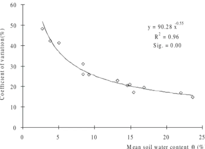
co-efficients of variation ranged from 14.9% to 48.2% (Table 1), indicating a moderate spatial variability of θ on the hillslope scale. The relationship between het-erogeneity of the variability and the soil moisture con-dition is shown through the plot of the coefficient of variation versus the mean θ (Figure 3). The coefficient of variation decreased exponentially with the mean θ, which indicates that the 0-6 cm soil moisture on the hillslope tends to be more homogeneous when the soil becomes wetter. The distribution of surface θ is in-fluenced by several factors, thus the change of the magnitude of the spatial variability of θ may reflect and also be the result of the evolution of dominating fac-tors in different soil moisture conditions.
Figure 2 - Soil water content (θ ) of the 0-6 cm soil layer along the toposequence during the observational period.
0 4 8 12 16 20 24 28 32
0 20 40 60 80 100 120 140 160 180 200 220 240 260 280
Distance along toposequence (m)
1183 1193 1203 1213 1223 1233 1243
May 17 May 18 May 20
May 22 May 26 May 29
May 31 June 2 June 5
June 8 June 11 June 15
June 21 E levation
Soi
l w
at
er
con
ten
t
(%
)
El
ev
at
io
n
(m
)
Figure 3 - Coefficients of variation versus 0-6 cm soil water content (θ ).
y = 90.2 8 x-0.55 R2 = 0 .96 S ig. = 0 .00
0 10 20 30 40 50 60
0 5 10 15 20 25
M ean soil w ater co ntent G (% )
C
oef
fi
ci
en
to
fv
ar
ia
ti
on
(%
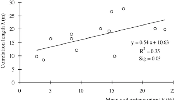
Soil moisture variability reflects to some ex-tent the variability of soil porosity, thus soil particle dis-tribution. Likewise, the variation of different particle sizes might explain the θ variability. For the particle classes ranging from 0.05-0.1 mm, the variability was larger for the finer particle class (Table 2). For the θ data of this study, the maximum mean is 23.63%, the soil sorptivity is between 10-20 kPa according to the retention curve of the local soil (Yang & Shao, 2000), and most of water is kept in pores sized within 0.015-0.03 mm of equivalent diameter. Generally, small pores tend to be formed by fine particles; therefore, it is not difficult to understand that the CV% increases when the soil dried out .In contrast, beyond the particle class of 0.05-0.1 mm, the variability is likely to be increased. Hence, if θ increases from a low value, as observed in this study, to a high value as saturation, then the vari-ability of θ might decrease first and then increase again. Correlation lengths λ for all the measurements are also listed in Table 1.The relationship between λ and θ (Figure 4) shows that λ increased linearly with the mean θ (P = 0.033), ranging from 8.4 to 27.7 m. This may imply that the extent over which correlation exists becomes larger as the soil becomes wetter. In other words, the surface θ tends to be much more
in-r e b m u
N Minimum Maximum Mean Standard
r o r r E d r a d n a t S n o i t a i v e D t n e i c i f f e o C n o i t a i r a V f
o Skewness Kurtosis
n o i t a l e r r o C * h t g n e L -% -- m 7 1 y a
M 177 11.2 32.4 22.02 0.28 3.75 17.04 -0.290 0.152 20.18(0.9768)
8 1 y a
M 177 8.3 27.7 16.90 0.25 3.31 19.60 0.119 0.468 27.69(0.9635)
0 2 y a
M 177 6.5 23.1 14.92 0.24 3.15 21.14 0.052 -0.089 26.54(0.9729)
2 2 y a
M 177 8.0 23.8 14.55 0.23 3.00 20.58 0.042 0.160 19.26(0.9865)
6 2 y a
M 177 3.4 17.0 8.37 0.20 2.61 31.17 0.395 0.153 18.05(0.9560)
9 2 y a
M 177 14.6 34.1 23.63 0.27 3.53 14.93 -0.124 -0.053 19.80(0.9714)
1 3 y a
M 177 6.3 21.4 13.16 0.23 3.02 22.96 -0.075 -0.241 20.11(0.9700)
2 e n u
J 177 3.5 16.2 9.20 0.18 2.38 25.82 0.071 0.250 12.11(0.9858)
5 e n u
J 177 8.1 23.3 15.42 0.20 2.67 17.28 -0.144 0.198 9.82(0.9764)
8 e n u
J 177 2.4 16.8 8.37 0.16 2.19 26.14 0.491 0.845 16.34(0.9604)
1 1 e n u
J 177 1.4 11.5 5.04 0.16 2.08 41.26 0.713 0.087 16.32(0.9283)
5 1 e n u
J 177 1.0 9.5 3.85 0.12 1.62 42.22 0.802 0.633 8.44(0.9517)
1 2 e n u
J 177 0.5 6.7 2.73 0.10 1.32 48.22 0.682 0.124 9.62(0.9549)
Table 1 - Classical statistics of the 0-6 cm soil water content (θ) data during the observational period.
*included in bracket is adjusted R2
e l c i t r a P ) m m ( s s a l
c <0.001
-1 0 0 . 0 2 0 0 . 0 -2 0 0 . 0 5 0 0 . 0 -5 0 0 . 0 1 0 . 0 -1 0 . 0 2 0 . 0 -2 0 . 0 5 0 . 0 -5 0 . 0 1 . 0 -1 . 0 2 . 0 -2 . 0 5 2 . 0 -5 2 . 0 5 . 0 -5 . 0 1 n o i t r o p o r P ) %
( 3.47 2.21 4.62 5.72 9.21 25.29 30.41 14.14 2.44 2.76 0.57
f o t n e i c i f f e o C ) % ( n o i t a i r a
V 72.7 40.8 35.6 32.6 31.2 30.8 23.6 80.1 111.8 173.7 100.3
Table 2 - Soil particle distribution and coefficients of variation.
dependent as the soil dries out. This is in accordance with the investigations of Grayson et al. (1997) who found dry catchment conditions being characterized by a stochastic moisture pattern, while wet catchment conditions showed a much more organized pattern. The evolution of λ along time can be explained by the prevalence of different soil moisture dynamics. Under wetter conditions, variable lateral water flow occurred on the larger area along slope, which can lead to a more organized pattern of soil moisture. As the soil dries out, however, upward evapotranspiration plays an increasingly important role in the soil surface
wa-Figure 4 - Correlation length (λ) versus mean 0-6 cm soil water content (θ ).
y = 0.54 x + 10.63 R2 = 0.35 Sig.= 0.03 0 5 10 15 20 25 30
0 5 10 15 20 25
Mean soil water content è (%)
ter movement, which, obviously, results in a greater independence from neighbor areas.
Factors influencing soil moisture distribution
Correlation analysis between soil moisture and to-pographic and soil properties - Under the
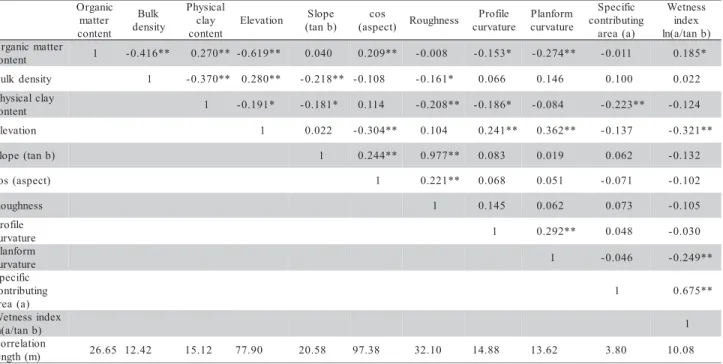
assump-tion that variaassump-tions in vegetaassump-tion, meteorological fac-tors and other significant influences on soil moisture variability are negligible at the hillslope scale, focus is given only on soil and topographic properties to iden-tify the dominating factors for soil moisture. Table 3 shows the Pearson’s correlation coefficients among topographic and soil characteristics as well as their correlation lengths, which indicate the existence of dif-ferent extents of correlation between soil and topo-graphic properties and their spatial structure.
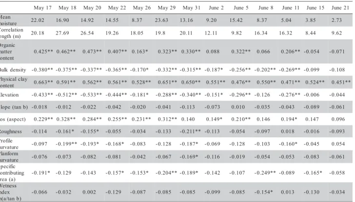
Pearson’s correlation coefficients for soil and topographic properties in relation to soil moisture ob-served on different dates (Table 4), indicate that for the same factors their correlation extent with θ can be quite different in terms of their significance level as well as the correlation sign. Generally, when disre-garding their significance level, soil organic matter con-tent, clay concon-tent, cos (aspect) were positively corre-lated with θ, while soil bulk density, elevation, slope (tan b), profile curvature, planform curvature, rough-ness, specifically contributing area, and wetness indexness (lna/tan b) were negatively correlated. When considering significance levels, however, profile cur-vature and planform curcur-vature were negatively corre-lated with θ only for observation dates 3 and 5 out of
the 13 dates, which agrees with Leij et al. (2004) who virtually found no correlation between retention param-eters and curvature of the land surface. For slope and roughness, although negatively correlation existed un-der all soil moistures of interest, significance can hardly be discovered. For the specific contributing area and wetness index, their negative correlations with θ, although not significant under most of the soil mois-ture conditions, may not be expected. The wetness in-dex and the specific contributing area are both nega-tively correlated with elevation (Table 3) and θ under all conditions were also negatively correlated with el-evation (Table 4). So, θ should be positively correlated with the wetness index and the specific contributing area, which is also an essentially normal phenomenon in θ estimation. However, the unexpected negative re-lation obtained in this study may imply in the fact that the wetness index and the specific contributing area may not be good estimators for the soil moisture dis-tribution at the semiarid hillslope scale.
Considering other factors such as aspect, el-evation, organic matter content, clay content, and soil bulk density it was found that for most soil water con-ditions (9 out of 13 at least), their correlations with soil moisture were significant. Among those, organic matter content, clay content, and cos (aspect) were in general positively correlated with θ, while soil bulk density and elevation were negatively linked to θ. Therefore, aspect, elevation, organic matter content, clay content, and soil bulk density are the main influ-encing factors on the θ distribution.
Table 3 - Pearson’s correlation coefficients among topographic and soil characteristics and their correlation lengths (λ). c i n a g r O r e t t a m t n e t n o c k l u B y t i s n e d l a c i s y h P y a l c t n e t n o c n o i t a v e l
E Slope
) b n a t ( s o c ) t c e p s a
( Roughness
e l i f o r P e r u t a v r u c m r o f n a l P e r u t a v r u c c i f i c e p S g n i t u b i r t n o c ) a ( a e r a s s e n t e W x e d n i ) b n a t / a ( n l r e t t a m c i n a g r O t n e t n o
c 1 -0.416** 0.270** -0.619** 0.040 0.209** -0.008 -0.153* -0.274** -0.011 0.185*
y t i s n e d k l u
B 1 -0.370** 0.280** -0.218** -0.108 -0.161* 0.066 0.146 0.100 0.022
y a l c l a c i s y h P t n e t n o
c 1 -0.191* -0.181* 0.114 -0.208** -0.186* -0.084 -0.223** -0.124
n o i t a v e l
E 1 0.022 -0.304** 0.104 0.241** 0.362** -0.137 -0.321**
) b n a t ( e p o l
S 1 0.244** 0.977** 0.083 0.019 0.062 -0.132
) t c e p s a ( s o
c 1 0.221** 0.068 0.051 -0.071 -0.102
s s e n h g u o
R 1 0.145 0.062 0.073 -0.105
e l i f o r P e r u t a v r u
c 1 0.292** 0.048 -0.030
m r o f n a l P e r u t a v r u
c 1 -0.046 -0.249**
c i f i c e p S g n i t u b i r t n o c ) a ( a e r a
1 0.675**
x e d n i s s e n t e W ) b n a t / a ( n l 1 n o i t a l e r r o C ) m ( h t g n e
l 26.65 12.42 15.12 77.90 20.58 97.38 32.10 14.88 13.62 3.80 10.08
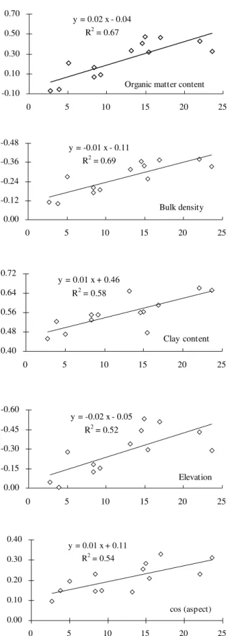
The relative importance of dominating factors in determining soil moisture distribution - The
dis-tinct correlation coefficients for aspect, elevation, or-ganic matter content, clay content, and soil bulk den-sity with θ under different observational data can be found in Table 4. Figure 5 characterizes the relation-ship of their correlation coefficients with mean θ, in-dicating that their magnitude of correlation increased with increasing values of θ (all passed the significant level test), no matter if negative or positive. Therefore, under higher soil moisture conditions, surface θ was much more controlled by the five main influencing fac-tors. Under lower soil moisture conditions, however, effects of these five main influencing factors were weaker, presenting no or adverse correlations when especially low soil moistures are considered, such as the average θ values of 3.85% on May 15 and of 2.73% on June 21. Therefore, with the drying pro-cess of the soil, θ may tend to be much more erratic rather than organized, echoed by the increasingly shorter correlation lengths (Figure 4).
Immediately after a rainfall event, it can be ex-pected that the soil bulk density (through porosity) would dominate the distribution of θ, which can be reflected by the larger negative correlation at higher soil moistures as compared with lower moisture con-ditions. Meanwhile, because of the high
evapotranspi-ration rates in this area, soil evapoevapotranspi-ration and plant tran-spiration would be the main active process soon after precipitation, and then organic matter and clay would control θ through their water retention ability. With the soil becoming drier, effects of organic matter and clay on θ became gradually negligible. In fact, since sam-pling was temporally lagged in relation to precipitation, the correlations of soil bulk density and soil moisture are far weaker than expected because of the dominat-ing process of soil evaporation that occurred soon af-ter that.
Aspect can influence the θ distribution by so-lar irradiance redistribution. At the beginning soil evapo-ration tends to be stronger and the influence of the as-pect would be largest. As the soil becomes drier, evaporation would decrease until minimum rates, and obviously, the effects of the aspect on θ distribution would also be decreased. This is in agreement with Hébrard et al. (2006) who did not find correlation be-tween the variation of insolation and the evolution of topsoil θ during the second drying sequence. Chanzy & Bruckler (1993) also pointed out that soil insolation was not the main factor controlling the dominant in-fluence when the soil was rather dry.
Elevation can exert large influence on soil mois-ture by its effects on the possible soil lateral flow along the slope. However, on this research area, possible lat-7
1 y a
M May18 May20 May22 May26 May29 May31 June2 June5 June8 June11 June15 June21
n a e M e r u t s i o
m 22.02 16.90 14.92 14.55 8.37 23.63 13.16 9.20 15.42 8.37 5.04 3.85 2.73
n o i t a l e r r o C ) m ( h t g n e
l 20.18 27.69 26.54 19.26 18.05 19.8 20.11 12.11 9.82 16.34 16.32 8.44 9.62
c i n a g r O r e t t a m t n e t n o c * * 5 2 4 .
0 0.462** 0.473** 0.407** 0.163* 0.323** 0.330** 0.088 0.322** 0.066 0.206** -0.054 -0.071
y t i s n e d k l u
B -0.380**-0.375** -0.337** -0.365** -0.170* -0.332**-0.315** -0.187* -0.256** -0.202** -0.269** -0.099 -0.108
y a l c l a c i s y h P t n e t n o
c 0.663** 0.591** 0.562** 0.561** 0.528** 0.651** 0.650** 0.551** 0.476** 0.550** 0.471** 0.524** 0.451**
n o i t a v e l
E -0.433**-0.512** -0.533** -0.444** -0.181* -0.288**-0.340** -0.151* -0.296** -0.126 -0.276** -0.006 -0.044
) b n a t ( e p o l
S -0.018 -0.012 -0.022 -0.042 -0.020 -0.041 -0.113 -0.073 0.010 -0.035 -0.043 -0.089 -0.061
) t c e p s a ( s o
c 0.229** 0.328** 0.284** 0.255** 0.231** 0.312** 0.140 0.149* 0.210** 0.146 0.194* 0.147 0.096
s s e n h g u o
R -0.114 -0.161* -0.155* -0.055 -0.034 -0.133 -0.211** -0.113 -0.054 -0.097 0.018 -0.016 -0.093
e l i f o r P e r u t a v r u
c -0.097 -0.199** -0.193* -0.168* -0.083 -0.128 -0.187* -0.069 -0.128 -0.103 -0.160* -0.045 0.054
m r o f n a l P e r u t a v r u
c -0.076 -0.073 -0.082 -0.081 -0.042 -0.067 -0.169* -0.116 -0.019 -0.054 -0.053 -0.083 -0.061
c i f i c e p S g n i t u b i r t n o c ) a ( a e r a * 1 9 1 . 0
- -0.129 -0.143 -0.157* -0.153* -0.204**-0.189* -0.142 -0.107 -0.249** -0.089 -0.165* -0.058
s s e n t e W x e d n i ) b n a t / a ( n l 6 6 0 . 0
- -0.032 0.002 -0.129 -0.087 -0.085 -0.085 -0.099 -0.085 -0.154* 0.013 -0.130 -0.034
Table 4 - Pearson’s correlation coefficients between 0-6 cm soil water content (θ) and topographic and soil characteristics during the entire observational period.
eral flow may soon be replaced by the strong evapo-ration, and therefore, no lateral flow at a dry condi-tion can explain the lower correlacondi-tion with θ under drier conditions. In addition, the increasingly weaker cor-relation between elevation and θ may also be the out-come of the combined effects of soil properties.
Many researchers have attempted to find out the real driving forces for θ distributions and, for this study, it seems unlikely to have success when con-sidering the complicated correlations among the vari-ous topographic and soil properties shown in Table 3. Taking elevation as an example, it is difficult to con-clude whether the significant correlation with θ is rep-resentative of the effects of its own or other soil prop-erties on θ. However, this may not be so important when choosing surrogates for θ distribution from the statistical point of view.
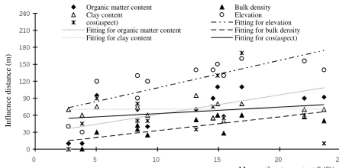
Cross-correlation analysis between soil moisture and dominating factors - With the aim of
understand-ing the effects of the five dominatunderstand-ing factors on the θ distribution with respect to its influencing area, cross-correlation coefficients were calculated for the five dominating factors with all θ observations. Figure 6 shows only the cross-correlograms of θ for May 17, which did not show symmetry with lag 0 (especially for elevation and aspect versus θ ), implying in a dif-ferent extent of influence in difdif-ferent directions. The absolute value of the cross-correlation coefficients of θ with all the dominating factors decreased with the lag distance increasing in both directions, which im-plies that the longer the distance separated by two vari-ables, the weaker the influence imposed by dominat-ing factors. As θ decreased, the cross-correlation co-efficients also exhibited a decreasing tendency for a given lag distance as occurred with the Pearson’s cor-relation coefficient (data not shown).
The lag distance coverage within which the cross-correlation coefficients have confidence limits was considered to be the influence distance. After es-timating the influence distance with cross-correlograms, the coefficients were plotted for all the dominating factors against mean θ (Figure 7), and as it can be seen, the influence distance for elevation, soil bulk density, and organic matter content increased ob-viously with mean θ, while those for clay content and aspect showed a slightly increasing tendency with θ. Therefore, in the process of drying, we can conclude that the factors influencing the decreasing effects on θ can be explained in two ways: (i.) their Pearson’s correlation coefficients as well as their cross-correla-tion coefficients with θ decreased with soil moisture; and (ii.) their influence distance on θ would be short-ened as well.
Figure 5 - Relationship between magnitude of the correlation and the mean soil water content (θ) (Abscissas denote the mean 0-6 cm soil water content θ, while ordinates are correlation coefficients).
Organic matter content y = 0.02 x - 0.04
R2 = 0.67
-0.10 0.10 0.30 0.50 0.70
0 5 10 15 20 25
Bulk density y = -0.01 x - 0.11
R2 = 0.69
-0.48
-0.36
-0.24
-0.12
0.00
0 5 10 15 20 25
Clay content y = 0.01 x + 0.46
R2 = 0.58
0.40 0.48 0.56 0.64 0.72
0 5 10 15 20 25
Elevation y = -0.02 x - 0.05
R2 = 0.52
-0.60
-0.45
-0.30
-0.15
0.00
0 5 10 15 20 25
cos (aspect) y = 0.01 x + 0.11
R2 = 0.54
0.00 0.10 0.20 0.30 0.40
Figure 6 - Cross-correlograms of the 0-6 cm soil water content (θ) for May 17 versus topographic and soil characteristics (Abscissas denote number of lag distance, while the ordinates are cross-correlation coefficients, confidence limits are also shown as dotted diamond line).
Soil moisture versus Organic matter content
-0.30 -0.15 0.00 0.15 0.30 0.45
-100 -80 -60 -40 -20 0 20 40 60 80 100
Soil moisture versus Bulk density
-0.45 -0.30 -0.15 0.00 0.15 0.30
-100 -80 -60 -40 -20 0 20 40 60 80 100
Soil moisture versus Clay content
-0.20 0.00 0.20 0.40 0.60 0.80
-100 -80 -60 -40 -20 0 20 40 60 80 100
Soil moisture versus Elevation
-0.60 -0.40 -0.20 0.00 0.20 0.40
-100 -80 -60 -40 -20 0 20 40 60 80 100
Soil moisture versus cos (aspect)
0.00 0.07 0.14 0.21 0.28 0.35
-100 -80 -60 -40 -20 0 20 40 60 80 100
Temporal stability analysis of soil moisture
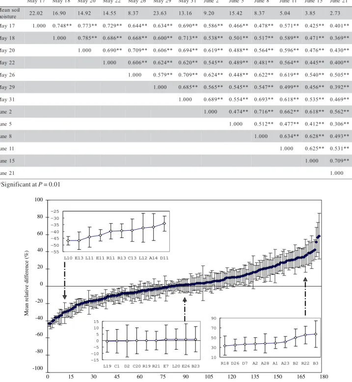
Spearman’s rank correlation coefficient analysis - The matrix of the rank correlation coefficients of θ for different dates during the entire measurement pe-riod is listed in Table 5. In general, the closer the rank correlation coefficient is to 1, the more stable is the process (Vachaud et al., 1985). All the values are highly significant (P = 0.01), indicating that a very strong time stability in the ranks of the locations can be assumed, as did Vachaud et al. (1985) and Pelt & Wierenga (2001).
Aspect, elevation, organic matter content, clay content, and bulk density were generally the main in-fluencing factors for the θ distribution for the differ-ent measuremdiffer-ent dates, although their influences weak-ened under dry conditions. Since these factors kept relatively invariable for a long time, the strong time sta-bility for θ for different dates becomes very clear. Based on soil water content measurements made with neutron probes, Reichardt et al. (1997) suggested that part of the time stability is due to the use of incorrect calibration curves. Generally, the same calibration curve is used over a whole field and due to the soil matrix variability, each sampling point is affected by a systematic error, or a systematic deviation from the mean. This might well also be true for FDR measure-ments, and has to be better explored in the future.
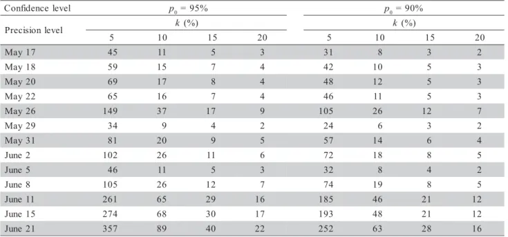
Relative difference analysis - After calculating the
time average of the relative differences and the tem-poral standard deviations for each location, the mean relative differences for θ were ranked from the small-est to the largsmall-est (Figure 8). Locations R19 and R21, with values close to 0 and with temporal standard de-viations below 15%, were considered representative of mean θ at any observational day. Similarly certain lo-cations systematically either overestimate (B2, R22, and B3) or underestimate (L10, E13, and L11) the hillslope average θ, regardless of the observation time.
Estimation for mean soil moisture
In this study, the techniques to obtain
accu-Figure 7 - Influence distances for five dominating factors on soil water content (θ) for different soil moisture conditions. 0
30 60 90 120 150 180 210 240
0 5 10 15 20 25
Mean soil water content θ (%) Organic matter content Bulk density
Clay content Elevation
cos(aspect) Fitting for elevation
Fitting for organic matter content Fitting for bulk density Fitting for clay content Fitting for cos(aspect)
In
fl
ue
nc
e di
st
an
ce
(
m
rate mean of surface θ is considered in two ways. First, the sampling number was obtained with no ex-act locations required for a reasonable estimation of mean θ, based on classical statistics. Second, the es-timate of mean θ was attempted with a limited sam-pling number, at fixed locations based on relative
dif-Table 5 - Rank correlation coefficients matrix for the 0-6 cm soil water content (θ) for different soil moisture conditions (dates).
7 1 y a
M May18 May20 May22 May26 May29 May31 June2 June5 June8 June11 June15 June21
l i o s n a e M
e r u t s i o
m 22.02 16.90 14.92 14.55 8.37 23.63 13.16 9.20 15.42 8.37 5.04 3.85 2.73
7 1 y a
M 1.000 0.748** 0.773** 0.729** 0.644** 0.634** 0.690** 0.586** 0.466** 0.478** 0.571** 0.425** 0.401**
8 1 y a
M 1.000 0.785** 0.686** 0.668** 0.600** 0.713** 0.538** 0.501** 0.517** 0.589** 0.471** 0.369**
0 2 y a
M 1.000 0.690** 0.709** 0.606** 0.694** 0.619** 0.488** 0.564** 0.596** 0.476** 0.430**
2 2 y a
M 1.000 0.606** 0.624** 0.620** 0.545** 0.489** 0.481** 0.564** 0.445** 0.400**
6 2 y a
M 1.000 0.579** 0.709** 0.624** 0.448** 0.622** 0.619** 0.540** 0.505**
9 2 y a
M 1.000 0.685** 0.565** 0.545** 0.547** 0.499** 0.456** 0.392**
1 3 y a
M 1.000 0.689** 0.554** 0.693** 0.618** 0.535** 0.469**
2 e n u
J 1.000 0.474** 0.716** 0.662** 0.618** 0.562**
5 e n u
J 1.000 0.512** 0.477** 0.412** 0.306**
8 e n u
J 1.000 0.634** 0.628** 0.493**
1 1 e n u
J 1.000 0.625** 0.531**
5 1 e n u
J 1.000 0.709**
1 2 e n u
J 1.000
**Significant at P = 0.01
Figure 8 - Ranked mean relative differences for the 0-6 cm soil water content θ (One standard deviation bars and sub-figures referring to minimum, middle, and maximum of the mean relative difference sites numbers are also shown.
-100 -80 -60 -40 -20 0 20 40 60 80 100
0 15 30 45 60 75 90 105 120 135 150 165 180
Rank
M
ea
n re
la
tive
di
ffe
rence
(%)
-55 -50 -45 -40 -35 -30 -25
L10 E13 L11 E11 R11 R13 C13 L12 A14 D11
10 30 50 70 90
R18 D26 D7 A2 A28 A1 A23 B2 R22 B3 -15
-10 -5 0 5 10 15
L19C1 D2 C20 R19 R21 E7 L20 E26 B23
ference analysis of soil moisture and the relationship between soil moisture and dominating factors.
Sampling number required for the estimation of mean soil moisture - The normality test of
the normal distribution (P > 0.05), and therefore equa-tion (4) can be used to calculate the sampling number required for the estimation of the mean θ under dif-ferent confidence levels and precision, for all measure-ment dates listed in Table 6. Two obvious trends ex-isted. The resulting sampling number obtained from equation (4) was generally larger for the 95% confi-dence level than for 90%, and the sampling number increased when the precision increased from 20% to 5%. The sampling number was intimately associated to the CV(%) of θ, since the CV(%) differed with the soil moisture condition, so that it is supposed that the sampling number for the estimation would be differ-ent according to the soil moisture condition. Sampling numbers for different soil moisture conditions (Figure 9), under a confidence level of 95% and a precision level of 5%, showed that the sampling number de-creased exponentially with increasing θ. Therefore, for the estimation of θ, much more samples have to be taken under dry conditions because of their stronger
l e v e l e c n e d i f n o
C p0 =95% p0=90%
l e v e l n o i s i c e r
P k (%) k (%)
5 10 15 20 5 10 15 20
7 1 y a
M 45 11 5 3 31 8 3 2
8 1 y a
M 59 15 7 4 42 10 5 3
0 2 y a
M 69 17 8 4 48 12 5 3
2 2 y a
M 65 16 7 4 46 11 5 3
6 2 y a
M 149 37 17 9 105 26 12 7
9 2 y a
M 34 9 4 2 24 6 3 2
1 3 y a
M 81 20 9 5 57 14 6 4
2 e n u
J 102 26 11 6 72 18 8 5
5 e n u
J 46 11 5 3 32 8 4 2
8 e n u
J 105 26 12 7 74 19 8 5
1 1 e n u
J 261 65 29 16 185 46 21 12
5 1 e n u
J 274 68 30 17 193 48 21 12
1 2 e n u
J 357 89 40 22 252 63 28 16
Table 6 - Number of samples for accurate measurement of soil water content (θ) for different soil moisture conditions (dates). heterogeneity. As a consequence, under especially dry conditions, such as the mean soil moistures of 5.04%, 3.85%, and 2.73%, the sampling number under a pre-cision of 5% was even much greater than the sam-pling that was actually taken (177 points). Consider-ing the large difference of samplConsider-ing numbers required for mean θ estimation, therefore, caution should be taken in relation to the initial θ values when choosing the input parameters for hydrological modeling.
Estimation of mean soil moisture - Using the RD
and the DF methods, surface mean θ was estimated us-ing different numbers of locations at the hillslope scale. Because aspect, elevation, organic matter content, clay content, and soil bulk density are the main influencing factors, these factors were chosen for the DF method. Figure 10 shows the relationship of estimated mean θ versus measured mean θ. Most of the points are close to the 1:1 line, indicating that the two methods can well estimate the mean soil water content.
Ordinarily, only one location whose mean rela-tive difference is closest to 0 and with the least stan-dard deviation is sufficient to estimate the mean soil moisture accurately (Grayson & Western, 1998). Con-sidering a location with no exact zero mean relative difference and the existence of a temporal standard deviation, more than one location have to be used to improve the accuracy of estimation by the RD method. Similarly, this is also true for the DF method. Figure 11 shows the absolute values of relative estimated er-rors for different locations employed for both meth-ods. The more locations are adopted, the more the ab-solute values of relative errors decrease, indicating an increasingly enhanced predictive ability. Beyond ten
lo-Figure 9 - Sampling number under different soil moisture conditions (When confidence level is 95%, and precision level is 5%).
y = 1253.33 x-1,10 R2 = 0.96
0 50 100 150 200 250 300 350 400 450
0 5 10 15 20 25
Mean soil water content θ (%)
Sig.= 0.00
S
am
pl
ing
num
be
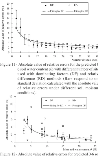
cations however, the predictive ability did not improve much as indicated by the extremely slow change of the absolute values of the relative errors. These rela-tive errors were small beyond ten locations, which were less than 5%.
Based on the knowledge of relatively poorer performance using ten locations in terms of estima-tion accuracy, only more than ten locaestima-tions were used to investigate the relative predictive ability under dif-ferent soil moisture conditions. Figure12 shows their relative predictive ability under different soil moisture conditions, and no matter which method used, their predictive ability tended to be better for wetter condi-tions, as indicated by the lower absolute value of the relative error for wetter conditions, which agrees well with Leij et al. (2004) who found more accurate pre-dictions for wetter conditions using Artificial Neural Networks. This may be related to the stronger spatial structure in wetter conditions and much more erratic distribution in drier conditions, as analyzed before. On this point, with the soil becoming drier, the decreased accuracy by both methods was in accordance with the increased number of samplings required for the esti-mation of the mean θ analyzed above.
As for the relative predictive ability of these two methods, the absolute value of the relative error for the DF method were less than that for the RD method, for most number of the locations, except for two or four locations as shown in Figure 11, and the absolute value of the relative error for the DF method was less than that for the RD method under lower soil moisture conditions. They were close to each other although a larger error of DF is shown as compared to RD (Figure 12). Results of samples compared by the T test with respect to absolute value of errors show that the predictive ability of the DF method was slightly better than the RD method, as indicated by the lower, not significant level of the absolute value of errors for the former method as compared to the latter method in Figure 11 (P = 0.216) and Figure 12 (P = 0.372).
Figure 10 - Measured versus predicted mean 0-6 cm soil water content (θ) with (a) dominating factors (DF) method and (b) relative difference (RD) method (Numeral in legend are the number of sites used to predict the mean soil water content).
0 5 10 15 20 25 30
0 5 10 15 20 25 30
2 4
6 8
10 12
14 16
18 20
22 24
26 28
30 32
34 36
38 40
1:1 line
In conclusion this study suggests an important implication for a realistic representation of soil mois-ture patterns in the context of distributed hydrological modeling at the hillslope scale. Specific emphasis should be given on issues closely related to the soil moisture condition, such as the magnitude of the vari-0
5 10 15 20 25 30
0 5 10 15 20 25 30
2 4
6 8
10 12
14 16
18 20
22 24
26 28
30 32
34 36
38 40
1:1 line
Predicted mean soil water content
G
(%)
Predicted mean soil water content
G
(%)
Measured mean soil water content G (%) Measured mean soil water content G (%)
Figure 11 - Absolute value of relative errors for the predicted 0-6 soil water content (θ) with different number of sites used with dominating factors (DF) and relative difference (RD) methods (Bars respond to one standard deviation calculated with the absolute value of relative errors under different soil moisture conditions).
0 2 4 6 8 10 12 14 16 18 20
0 4 8 12 16 20 24 28 32 36 40
Number of sites used
DF RD
Fitting for DF Fitting for RD
Ab
so
lu
te
v
al
ue
o
f re
la
tiv
e e
rro
rs
(%
)
Figure 12 - Absolute value of relative errors for predicted 0-6 soil water content (θ) with dominating factors (DF) and relative difference (RD) methods under different soil moisture conditions (Bars respond to one standard deviation calculated with the absolute value of relative errors under different number of sites ranging from 10 to 40 used to predict θ).
0 2 4 6 8 10 12
0 5 10 15 20 25
Mean soil water content è (%)
DF RD
Fitting for RD Fitting for DF
A
bs
ol
ute
va
lu
e o
f rel
ativ
e
erro
rs
(%
ability, spatial pattern, and different acting processes. Further work in this semiarid area should be oriented towards larger temporal and spatial scales with the aim of providing detailed knowledge for hydrological mod-eling.
ACKNOWLEDGEMENTS
To the "Innovation Team" program of the Chi-nese Academy of Sciences (Soil and water processes modeling in watersheds) and to the National Natural Sciences Foundation of China (Grant numbers of 90502006 and 50479063) and the “Hundred Talents Program” of the Chinese Academy of Sciences for the financial supports.
REFERENCES
CHANZY, A.; BRUCKLER, L. Significance of soil surface moisture with respect to bare soil evaporation. Water Resources Research, v.29, p.1113-1125, 1993.
FAMIGLIETTI, J.S.; RUDNICKI, J.W.; RODELL, M. Variability in surface moisture content along a hillslope transect: Rattlesnake Hill, Texas. Journal of Hydrology, v.210, p.259-281, 1998. GRAYSON, R.B.; WESTERN, A.W.; CHIEW, F.H.S.; BLÖSCHL, G. Preferred states in spatial soil moisture patterns: Local and nonlocal controls. Water Resources Research, v.33, p.2897-2908, 1997.
GRAYSON, R.B.; WESTERN, A.W. Towards areal estimation of soil water content from point measurements: time and space stability of mean response. Journal of Hydrology, v.207, p.68-82, 1998.
HAWLEY, M.E.; JACKSON, T.J.; McCUEN, R.H. Surface soil moisture variation on small agricultural watersheds. Journal of Hydrology, v.62, p.179-200, 1983.
HAWLEY, M.E.; McCUEN, R.H.; JACKSON, T.J. Volume-accuracy relationships in soil moisture sampling. Journal of the Irrigation and Drainage. v.108(IRI1), p.1-11, 1982. HÉBRARD, O.; VOLTZ, M.; ANDRIEUX, P.; MOUSSA, R.
Spatial-temporal distribution of soil surface moisture in a heterogeneously farmed Mediterranean catchment. Journal of Hydrology, v.329, p.110-121, 2006.
HU, W.; SHAO, M.A.; WANG, Q. J. Study on spatial variability of soil moisture on the recultivated slope-land on the Loess Plateau. Advances in Water Science, v.17, p.74-81, 2006. LEIJ, F.J.; ROMANO, N.; PALLADINO, M.; SCHAAP, M.G.;
COPPOLA, A. Topographical attributes to predict soil hydraulic properties along a hillslope transect. Water Resources Research, v.40, W02407, 2004.
NIELSEN, D.R.; WENDROTH, O. Spatial and temporal statistics. Reiskirchen: Catena, 2003. p.31-90.
PELT, R.S. van; WIERENGA, P.J. Temporal stability of spatially measured soil matric potential probability density function. Soil Science Society of American Journal, v.52, p.363-368, 2001.
REICHARDT, K.; PORTEZAN, O.; BACCHI, O.O.S.; OLIVEIRA, J.C.M.; DOURADO-NETO, D.; PILOTTO, J.E.; CALVACHE, M. Neutron probe calibration correction through temporal stability parameters of the soil water probability function. Scientia Agricola, v.54 (Special issue), p.17-21, 1997. REYNOLDS, S.G. The gravimetric method of soil moisture
determination. III. An examination of factors influencing soil moisture variability. Journal of Hydrology, v.11, p.288-300, 1970.
SHAO, M.A.; WANG, Q.J.; HUANG, M.B. Soil physics. Beijing: Higher Education Press, 2006. p.16-21.
STARKS, P.J.; HEATHMAN, G.C.; JACKSON, T.J.; COSH, M.H. Temporal stability of soil moisture profile. Journal of Hydrology, v.324, p.400-411, 2006.
TANG, K.L.; HOU, Q.C.; WANG, B.K.; ZHANG, P.C. The environment background and administration way of wind-water erosion crisscross region and Shenmu experimental area on the Loess Plateau. Memoir of NISWC, Academia Sinica and Ministry of Water Conservation, v.18, p.2-15, 1993. TIMM, L.C.; PIRES, L.F.; ROVERATTI, R.; ARTHUR, R.C.J.;
REICHARDT, K.; OLIVIRA, J.C.M.; BACCHI, O.O.S. Field spatial and temporal patterns of soil water content and bulk density changes. Scientia Agricola, v.63, p.55-64, 2006. VACHAUD, G.; PASSERAT DE SILANS, A.; BALABANIS, P.;
VAUCLIN, M. Temporal stability of spatially measured soil water probability density function. Soil Science Society of American Journal, v. 49, p.822-828, 1985.
WESTERN, A.W.; BLÖSCHL, G. On the spatial scaling of soil moisture. Journal of Hydrology, v.217, p.203-224, 1999. WESTERN, A.W.; GRAYSON, R.B.; BLÖSCHL, G. Scaling of soil
moisture: a hydrologic perspective. Annual Review of Earth and Planetary Sciences, v.205, p.20-37, 2002.
WESTERN, A.W.; ZHOU, S.L.; GRAYSON, R.B.; McMAHON, T.A.; BLÖSCHL, G.; WILSON, D.J. Spatial correlation of soil moisture in small catchments and its relationship to dominant spatial hydrological processes. Journal of Hydrology, v.286, p.113-134, 2004.
YANG, W.Z.; SHAO, M.A. Study on soil moisture on the Loess Plateau. Beijing: Science Press, 2000. p.134-172.