www.ocean-sci.net/11/629/2015/ doi:10.5194/os-11-629-2015
© Author(s) 2015. CC Attribution 3.0 License.
Eddy surface properties and propagation at Southern Hemisphere
western boundary current systems
G. S. Pilo1,a, M. M. Mata1, and J. L. L. Azevedo1
1Laboratorio de Estudos dos Oceanos e Clima, Instituto de Oceanografia, Universidade Federal do Rio Grande (FURG), Rio Grande, Rio Grande do Sul, Brasil
anow at: Institute for Marine and Antarctic Studies, University of Tasmania, and CSIRO Oceans and Atmosphere Flagship, Tasmania, Australia
Correspondence to:G. S. Pilo ([email protected])
Received: 6 January 2015 – Published in Ocean Sci. Discuss.: 9 February 2015 Revised: 30 June 2015 – Accepted: 2 August 2015 – Published: 12 August 2015
Abstract.Oceanic eddies exist throughout the world oceans, but are more energetic when associated with western bound-ary currents (WBC) systems. In these regions, eddies play an important role in mixing and energy exchange. There-fore, it is important to quantify and qualify eddies associated with these systems. This is particularly true for the South-ern Hemisphere WBC system where only few eddy censuses have been performed to date. In these systems, important as-pects of the local eddy population are still unknown, like their spatial distribution and propagation patterns. Moreover, the understanding of these patterns helps to establish mon-itoring programs and to gain insight in how eddies would affect local mixing. Here, we use a global eddy data set to qualify eddies based on their surface characteristics in the Agulhas Current (AC), the Brazil Current (BC) and the East Australian Current (EAC) systems. The analyses reveal that eddy propagation within each system is highly forced by the local mean flow and bathymetry. Large values of eddy am-plitude and temporal variability are associated with the BC and EAC retroflections, while small values occur in the cen-tre of the Argentine Basin and in the Tasman Sea. In the AC system, eddy polarity dictates the propagation distance. BC system eddies do not propagate beyond the Argentine Basin, and are advected by the local ocean circulation. EAC system eddies from both polarities cross south of Tasmania but only the anticyclonic ones reach the Great Australian Bight. For all three WBC systems, both cyclonic and anticyclonic ed-dies present a geographical segregation according to radius size and amplitude. Regions of high eddy kinetic energy are associated with the eddies’ mean amplitudes, and not with their densities.
1 Introduction
Oceanic mesoscale eddies are defined by a closed circula-tion (Cushman-Roisin and Beckers, 2006), having an inter-nal water parcel with different characteristics from the sur-rounding fluid (Flierl, 1979). Due to their advective proper-ties, eddies play an important role in ocean circulation. Ed-dies redistribute heat, salt, and momentum between different regions and mix and exchange energy with the mean flow (e.g. Stammer and Wunsch, 1999; Lee et al., 2007). Despite being found in all oceans, eddies are most intense when as-sociated with western boundary currents (WBCs) (Chelton et al., 2011). In these highly energetic regions, eddies often originate from mean flow instabilities being shed by the cur-rents’ meanders.
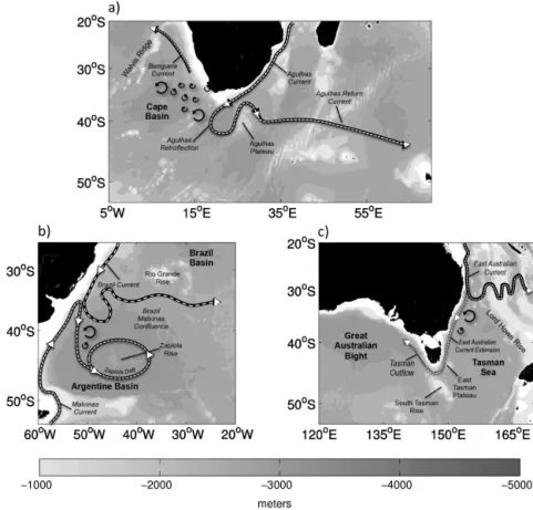
Figure 1. Main bathymetric features and circulation patterns of the(a)AC,(b) BC and(c)EAC systems (adapted from Peterson and Stramma, 1991, Cresswell, 2000, Tilburg et al., 2001, Mata et al., 2006, Matano et al., 2010).
In the AC system, censuses of large anticyclonic eddies were extensively performed using sea surface temperature data (Lutjeharms and Van Ballegooyen, 1988) and single-satellite altimetry data (e.g. Byrne et al., 1995; Goni et al., 1997; Schouten et al., 2000). Censuses of large cyclonic eddies in the region were performed using merged altime-try products (e.g. Boebel et al., 2003; Hall and Lutjeharms, 2011). These studies show that large retroflection anticy-clonic eddies propagate beyond Cape Basin, while cyanticy-clonic eddies remain trapped within it. These censuses, while pre-senting insightful results for eddies in the Cape Basin and AC retroflection region, omit the ARC region.
In the BC system, eddy censuses were performed us-ing sea surface temperature data (Legeckis and Gordon, 1982; Lentini et al., 2002) and single-satellite altimetry data (Lentini et al., 2006). These early studies were based on data with reduced temporal and spatial resolution; therefore, the sample of eddies is biased towards large, persistent features. The 67 eddies considered in these studies propagate in a disorganised manner, close to the Brazil–Malvinas Conflu-ence (BMC), being later reabsorbed by their parent current. A census using merged altimetry data was also performed in the Argentine Basin, the bathymetric feature in which the BC retroflection and the BMC are located (Fig. 1). There, eddy shedding is associated with meandering of the local
anticy-clonic flow, called the Zapiola Drift (Saraceno and Provost, 2012). It is still unknown if eddies shed by the BC, the BMC or the Zapiola Drift propagate beyond the Argentine Basin. Their mean lifetime and surface properties also require fur-ther assessment.
In the EAC system, Everett et al. (2012) studied eddies with a global eddy data set (Chelton et al., 2011) built from altimetry data. These authors show that a large number of eddies occur close to the Australian shelf break between the retroflection region (∼31◦S) and the east coast of
Tasma-nia (∼40◦S). However, they do not investigate lifetimes or
propagation of eddies.
As shown above, previous studies performed eddy cen-suses in the three systems of interest. However, important aspects of local eddy fields remain unknown. The main ques-tions still to be answered relate to spatial distribution and propagation of eddies within each system. In that sense, the goal of this research is to qualify the AC, BC and EAC sys-tem eddies based on their surface properties (i.e. amplitude, radius, rotation speed) and investigate eddy propagation and spatial distribution.
cm2/s2
Number of eddies a) Eddy Kinetic Energy
b) Eddy density
AC
BC
MC
ZA
EAC
EAC AC
BC
MC
ZA
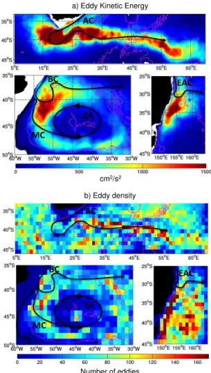
Figure 2. (a)Mean eddy kinetic Energy between January 1993 and
December 2011 and(b)total number of eddies occurring in each
1◦×1◦ cell between October 1992 and April 2012 in the AC, BC
and EAC systems.
monitoring programs (i.e. moorings location, hydrographic sampling). Also, it helps us to better understand the eddies’ contribution to oceanic heat and salt transports and how ed-dies affect local mixing.
The next section describes the global eddy data set used in this study as well as our investigation methods. In Sect. 3 we show the eddy density, radius and amplitude spatial distri-bution in all systems. We also show eddy mean propagation and mean properties (i.e. amplitude, radius, rotation speed, lifetime). In Sect. 4 we discuss the results and in Sect. 5 we summarise our main findings.
2 Data and methods 2.1 The eddy data set
We use version 3 global eddy data set of D. Chelton and M. Schlax (Chelton et al., 2011; available at http://cioss.coas. oregonstate.edu/eddies/). This data set provides eddy tracks
identified in global merged sea surface height (SSH) maps between October 1992 and April 2012. Eddy radius, ampli-tude and rotation speed are also provided at each time step of the eddy lifetime. The SSH maps used to build this data set have weekly temporal resolution and, after filtering, 0.25◦ spatial resolution (see Chelton et al., 2011 Appendix A); therefore, most of the mesoscale spectrum is resolved. The eddies are identified using a SSH-based method and tracked using the same approach as Chelton et al. (2007). We refer the reader to Chelton et al. (2011) for further information on the identification and tracking method.
Here, we select eddies with first occurrences (i.e. first de-tections) in (a) the Agulhas Retroflection and the ARC (33– 46◦
S and 5–70◦
E), hereafter defined as the AC system (the region comprised in Fig. 2a); (b) the Argentine Basin, as-sociated with the BMC and the BC retroflection (35–50◦S, 60–30◦W), hereafter defined as the BC system (the region comprised in Fig. 2a); and (c) the EAC, flowing through western regions of the Coral and the Tasman seas, and the current’s retroflection (25–45◦
S, 147–164◦
E), hereafter de-fined as the EAC system (the region comprised in Fig. 2a). In the AC system we do not include eddies from the Mozam-bique Channel (north of the study region) and from the East Madagascar Current (to the east of the study region). These eddies may affect eddy shedding by the Agulhas Retroflec-tion (Lutjeharms, 2006). However, in the data set used here, no eddy formed in these regions reach either the Cape Basin or the ARC (not shown) and seem to belong to different en-ergy systems.
One must consider aspects of the global eddy data set when investigating its output. One relevant aspect for our study is the premature eddy dissipation due to detection in-accuracies. Eddies can escape detection in sparsely sam-pled regions (i.e. between satellite ground tracks), where the gridded altimetry data set has reduced spatial resolu-tion. Eddies can also escape detection after merging, split-ting, and interacting with other eddies, the mean flow and local bathymetry. These events can distort the eddy, failing to satisfy the algorithm identification criteria. An eddy can be later re-identified and considered as a new eddy. There-fore, detection inaccuracies may not only lead to premature dissipation but also to late detection and, more importantly, tagging of “old” eddies as new ones.
There-fore, only eddies originated in our study regions with life-times longer than 10 weeks are considered.
2.2 Maps of eddy properties
We build spatial distribution maps of eddy properties (radius, mean propagation, and amplitude), as well as eddy density and eddy kinetic energy (EKE) maps for each of the study regions.
Eddy mean and standard deviation (SD) radius and am-plitude maps are built after gridding each WBC region onto 1◦×
1◦
cells. We then consider the radius and amplitude of all eddy-like features (lifetime > 4 weeks) that occur in each cell to calculate both mean and SD values for that cell. This analysis is performed throughout the entire time series (Octo-ber 1992–April 2012). To test for significance of mean values we perform a non-pairedt test with 95 % confidence level. To determine eddies with mean radii and amplitudes larger (smaller) than the mean within that system we perform a right (left) tail test.
Eddy density maps are built by considering how many eddies with lifetimes > 10 weeks are identified within each 1◦
×1◦
grid cell. These maps relate to individual observa-tions of eddies, instead of individual eddies. For example, if an eddy is stationary within a cell for 3 weeks, it will count as three eddy observations within that cell.
Eddy mean propagation maps are built by considering the mean propagation speed of eddies with lifetimes > 10 weeks within each 1◦×
1◦
grid cell. To achieve that, we select grid cells that contain more than 20 eddies and calculate these eddies’ speeds from their location within this cell at timetto their next location at timet+1. We then calculate the mean propagation speed by considering the propagation speed of all eddies within that cell.
Mean EKE maps are built using Aviso’s Reference Se-ries Maps of Absolute Geostrophic Velocities between Jan-uary 1993 and December 2010 (http://www.aviso.altimetry. fr/duacs/).
2.3 Eddy mean properties
To calculate an eddy mean surface property along its lifetime we first multiply the property mean between two subsequent time steps by the distance the eddy propagates in this time period (i.e. 7 days). Then, these adjacent time-step products from the entire eddy lifetime are summed. This sum is then divided by the total distance that the eddy covered along its lifetime. We repeat this procedure for all eddies within the same system.
3 Results
3.1 Eddy kinetic energy and eddy density
The EKE is a measurement of mesoscale activity within a re-gion. Therefore, one would expect regions with high EKE to be associated with an increased number of eddies. With that in mind, we look at both mean EKE maps and eddy density maps of the three systems (Fig. 2a, b, respectively). While high mean EKE is associated with the WBCs retroflection regions, high eddy density seems not to be the case.
In the AC system, high mean EKE values occur in the AC retroflection (∼17◦
E, 37◦
S) and expand further west, reaching the Cape Basin. In this system the ARC also dis-plays high EKE values along its path. Here, the meander-ing performed by the current when encountermeander-ing the Agulhas Plateau (26◦
E, 40◦
S) becomes evident. High eddy density patterns do not agree with the EKE distribution in this sys-tem, with eddies occurring over the entire region. Cells with low eddy density occur both to the north and to the south of the ARC.
In the BMC system, high mean EKE values occur in the BC retroflection (∼52◦W, 40◦S) and contouring the
Argen-tine Basin, as previously shown by Fu (2006). High eddy density patterns do not agree to the mean EKE distribution in this system. High density cells occur in the outer portions of the basin and over the Zapiola Rise, a bathymetric fea-ture in the centre of the Argentine Basin (45◦
W, 45◦ S) that rises up to 4700 m below the surface (Ewing, 1964). This basin has depths exceeding 6000 m in its southwestern part (Saunders and King, 1995). This high eddy density over the Zapiola Rise was previously shown by Saraceno and Provost (2012) to be due to the presence of cyclonic eddies that enter the Zapiola Drift. This drift is an anticyclonic flow that dom-inates the Argentine Basin circulation (Miranda et al., 1999), flowing around the Zapiola Rise.
In the EAC system, high mean EKE values occur to the south of the EAC retroflection (∼157◦E, 31◦S) extending to
the southern end of Australia’s mainland. However, a band of high eddy density cells expand further south, reaching Tas-mania. Eddies also occur over the entire Tasman Sea and not only close to the eastern Australian shelf break, as suggested by the mean EKE map.
3.2 Mean eddy radius and amplitude spatial distribution
As we can see, there is more to the high values of mean EKE in these three systems than the abundance of eddies. To further understand the spatial distribution of eddies, Fig. 3 shows the horizontal length (radius) and amplitude occurring over these regions.
60oW 55oW 50oW 45oW 40oW 35oW 30oW 50oS
45oS 40oS 35oS
150oE 155oE 160oE 45oS
40oS 35oS 30oS 25oS
b) Eddy Amplitude
5oE 15oE 25oE 35oE 45oE 55oE 65oE 45oS
40oS 35oS
5 10 15 20 25 30 35 40
60oW 55oW 50oW 45oW 40oW 35oW 30oW 50oS
45oS 40oS 35oS
150oE 155oE 160oE 45oS
40oS 35oS 30oS 25oS a) Eddy Radius
5oE 15oE 25oE 35oE 45oE 55oE 65oE 45oS
40oS 35oS
40 50 60 70 80 90 100 110 120 130
Figure 3.Mean(a)radii (km) and(b) amplitudes (cm) of
eddy-like features (lifetime > 4 weeks) in the AC, BC and EAC systems
in a 1◦×1◦ grid, with magenta lines indicating the 4000, 3000 and
2000 m isobaths, respectively. White (black) stars indicate cells with values significantly smaller (higher) than the system mean.
and amplitudes (Fig. 3b) occur to the south of the ARC. The distribution of eddies with large radii and large amplitudes agrees with the mean EKE distribution in Fig. 2a. Therefore, the mean EKE, eddy radius and eddy amplitude distributions all match in this system, meaning that large radius eddies are also the most energetic ones.
The BC system eddies’ radius (Fig. 3a) and amplitude (Fig. 3b) spatial distributions do not match. Eddies with sig-nificantly larger radii occur in the entire northern domain of the Argentine Basin, while eddies with significantly larger amplitudes cluster in the BC retroflection region (∼55◦
W, 41◦
S). Eddies with significantly smaller radii and amplitudes coexist in the centre of the Argentine Basin. Here, eddies’ amplitudes spatial distribution relates better to mean EKE distribution (Fig. 2a) than to the eddies’ radii distribution.
EAC system eddies with significantly larger radii (Fig. 3a) and amplitudes (Fig. 3b) only overlap near the current’s
60oW 55oW 50oW 45oW 40oW 35oW 30oW 50oS
45oS
40oS 35oS
150oE 155oE 160oE
45oS
40oS 35oS
30oS 25oS
a) Eddy radius standard deviation
5oE 15oE 25oE 35oE 45oE 55oE 65oE 45oS
40oS
35oS
16 18 20 22 24 26 28 30 32
60oW 55oW 50oW 45oW 40oW 35oW 30oW 50oS
45oS 40oS 35oS
150oE 155oE 160oE 45oS
40oS 35oS 30oS 25oS
b) Eddy amplitude standard deviation
5oE 15oE 25oE 35oE 45oE 55oE 65oE 45oS
40oS 35oS
5 10 15 20
km
cm
a) Eddy radius standard deviation
b) Eddy amplitude standard deviation
Figure 4.Standard deviation of (a)radii (km) and(b)amplitude
(cm) of eddy-like features (lifetime > 4 weeks) in the AC, BC and
EAC systems in a 1◦×1◦ grid, with magenta lines indicating the
4000, 3000 and 2000 m isobaths, respectively.
retroflection region (∼ 31◦S), which is also where mean
EKE is higher in this system (Fig. 2a). Again, high mean EKE values relate better to eddy amplitude distribution than to eddy radius. Eddies with significantly larger radii occur in the Coral Sea, north of the EAC separation region. Eddies with significantly smaller radius occur in the Tasman Sea.
Moreover, the spatial patterns in Fig. 3 are very similar to both cyclonic and anticyclonic eddies (not shown). There-fore, we chose to combine both polarities in the making of the figures.
3.3 Eddy radius and amplitude spatial variability Maps of the eddies’ radius and amplitude SDs give us fur-ther insight into these properties and their spatial pattern of variability (Fig. 4).
Figure 5.Trajectories of(a)cyclonic, and(b)anticyclonic eddies first identified in the AC system between October 1992 and April 2012.
Insets in(a)and(b)show the South Atlantic crossing eddies’ first locations.
me
ters
a)
b)
Figure 6.Trajectories of(a)cyclonic and(b)anticyclonic eddies
first identified in the BC system between October 1992 and April 2012.
similar to eddy mean radius emerge both in the BC and the EAC systems. In the BC system cells with high standard de-viation values cluster in the northeast domain of the basin. In the EAC system most of the variability happens in the cur-rent’s retroflection region.
Eddy amplitude SD spatial distributions for all systems are similar to the eddy mean amplitude distribution (Fig. 4b). Here, cells with high SD values are associated with the AC, the BC and the EAC retroflections.
3.4 Eddy propagation
To investigate the propagation of eddies within and beyond each system we look at both individual eddy tracks (Figs. 5, 6, 7) and maps of mean propagation within 1◦
×1◦
cells (Fig. 8). While the individual tracks of eddies give us insight into the general eddy distribution, mean propagation maps show a clearer picture.
3.4.1 Agulhas Current system
In the AC system 2740 eddies are identified, 48 % of them being cyclonic and 52 % of them anticyclonic. Both cyclonic and anticyclonic eddies occur over the entire domain, except over the continental shelf (Fig. 5a, b). Some eddies propagate beyond the domain, reaching as far as 50◦
W when propagat-ing westward and 75◦
E when propagating eastward. Both cyclonic and anticyclonic eddies propagate beyond the Cape Basin. Three cyclonic eddies overcome the Walvis Ridge, with one propagating 5000 km across the South At-lantic. This cyclonic eddy reaches the Rio Grande Rise, at
∼40◦W, before dissipating (i.e. being lost by the algorithm). More anticyclonic eddies propagate beyond the AC system into the South Atlantic than cyclonic ones. A total of 24 anti-cyclonic eddies reach the Brazilian continental shelf break. These eddies originate in the Cape Basin (Fig. 5b, inset). While in the Cape Basin, they propagate along the “eddy cor-ridor” defined by Goni et al. (1997) between 25 and 42◦
S. As they propagate into the Atlantic they are located between 20 and 30◦
Figure 7.Trajectories of(a)cyclonic and(b)anticyclonic eddies first identified in the EAC system between October 1992 and April 2012. Eddy tracks that cross south of Tasmania are shown in black.
the South Atlantic corroborates to ones previously shown in the literature (Fu, 2006; Souza et al., 2011; Azevedo et al., 2012).
When looking at the mean propagation of eddies in the AC system, two westward patterns are dominant (Fig. 8): in the Cape Basin and north of the ARC. In the Cape Basin ed-dies propagate as fast as 7 cm s−1. Here, the “eddy corridor” is well defined by higher propagation speeds. After leaving the Cape Basin, eddies still present high mean propagation in the South Atlantic. North of the ARC, in the Indian Ocean, eddies propagate at∼4 cm s−1. Two smaller patches of east-ward mean velocities are centred at 47◦
E, 47◦
S and at 70◦ E, 45◦
S. The northern one is caused by ARC advection and the southern by Antarctic Circumpolar Current advection. 3.4.2 Brazil Current system
In the BC system 1119 eddies are identified, 56 % of them being cyclonic and 44 % of them anticyclonic. Both cyclonic and anticyclonic eddies propagate strictly within the Argen-tine Basin (Fig. 6), and eddy numbers are small where the Zapiola Drift is most intense.
Here, we see three eddies identified over the continental shelf. These eddies should be considered with caution. Ac-cording to Saraceno and Provost (2012), altimeter data on
the Patagonian shelf are usually unreliable due to intrinsic difficulties on corrections applied to data, especially related to tides. In their study, where they perform an eddy census in the Argentine Basin using gridded altimetry data, they only consider eddies identified offshore (i.e. depths greater than 200 m).
Cyclonic eddies occur over the entire basin, also dominat-ing the inner portion of the Zapiola Drift (Fig. 6a). There, 23 cyclonic eddies display an anticlockwise propagation around the Zapiola Rise, entering the drift on its eastern flank. On average, two cyclonic eddies entered the drift per year be-tween 1998 and 2011; however, none is detected after this period. In turn, anticyclonic eddies occur in the boundaries of the Argentine Basin. Only a few tracks occur in the inner part of the Zapiola Drift.
Eddies located along the Argentinian continental shelf break and propagate northward, with mean speeds between 3 and 7 cm s−1(Fig. 8;∼55◦W, 47◦S). These northward ed-dies are probably being advected by the Malvinas Current. This current flows northward along the slope at 40 cm s−1 (Peterson, 1992), therefore, with higher speeds than the ed-dies’ mean speed at that location. However, the intrinsic westward propagation of eddies might be slowing the Malv-inas Current advection down. The effect of the Zapiola Drift on the remaining BC system eddies is clear.
3.4.3 East Australian Current system
In the EAC system 1050 eddies are identified, 51 % of them being cyclonic and 49 % of them anticyclonic. The eddies occur over the entire domain, clustering off the continental shelf break (Fig. 7). This clustering contains eddies shed by the EAC retroflection and eddies travelling westward from the Tasman Sea. Roughly 88 % of the EAC system eddies propagate westward.
Both cyclonic and anticyclonic EAC system eddies can cross south of Tasmania and reach the Great Australian Bight (Fig. 7, in black). These eddies are first identified east of Tas-mania. The 10 anticyclonic eddies that cross south of Tasma-nia have a mean radius of 70 km and mean lifetime of 1.5 years, living up to 5 years.
Over most of the EAC system, eddies propagate west-ward (Fig. 8) and, when encountering the eastern Australian shelf slope, they turn southward. Higher propagation speeds (∼3–6 cm s−1) are found in the Coral Sea and close to the EAC retroflection region. In the Tasman Sea eddies prop-agate slower (1–2.5 cm s−1). It is relevant to say that these propagation speeds within each cell do not denote eddy track continuity but denote a mean pattern of propagation for ed-dies occurring at each location.
3.5 Eddy mean properties
60oW 55oW 50oW 45oW 40oW 35oW 30oW
50oS
45oS
40oS
35oS
145oE 151oE 157oE 163oE
45oS
40oS
35oS
30oS
25oS
30oW 10oW 10oE 30oE 50oE 70oE
45oS
40oS
35oS
30oS
25oS
0 0.01 0.02 0.03 0.04 0.05 0.06 0.07
m/s
a)
b)
b)
c)
Figure 8.Eddy mean propagation speeds (colours) and directions (arrows) for 1◦×1◦cells containing more than 20 eddies in the(a)AC,
(b)BC, and(c)EAC systems.
Table 1.Mean (and SD) properties and characteristics of cyclonic (Cyc) and anticyclonic (Anti) long-lived eddies. See text for description
of mean calculation.
Mean (SD)
AC system BC system EAC system
Cyc Anti Cyc Anti Cyc Anti
Propagation distance 732.8 1050.4 523.4 513.8 521.5 522.2
(km) (640.5) (1258.0) (282.6) (263.9) (374.9) (427.1)
Propagation speed 4.0 3.8 4.4 4.6 3.2 3.1
(km day−1) (1.3) (1.3) (1.5) (1.7) (1.2) (1.1)
Lifetime 26.3 37.2 17.3 16.3 22.9 24.6
(weeks) (21.6) (38.6) (8.3) (7.5) (14.9) (19.8)
Amplitude 8.9 7.9 18.7 15.9 9.2 8.6
(cm) (8.1) (6.0) (9.0) (7.8) (7.1) (6.4)
Rotation speed 19.5 17.5 31.7 29.4 21.1 20.1
(cm s−1) (13.9) (9.9) (12.0) (11.4) (13.7) (12.5)
Radius 87.0 89.0 87.6 90.7 83.4 82.7
icant between cyclonic and anticyclonic eddies in all three systems (with some standard deviation values as large as the mean values). The similarities between cyclonic and anticy-clonic eddies is due to the large range of eddies investigated. Eddies with radii spanning from 40 to 130 km were included in the analysis.
Anticyclonic eddies from the AC system are the longer lived ones from all systems, due to their propagation across the South Atlantic. The small number of eddies propagating south of Tasmania do not increase the mean lifetime of EAC system anticyclonic eddies.
We draw attention to the BC system eddies’ shorter mean lifetimes and larger mean amplitudes when compared to the other systems. These differences occur because AC and EAC system eddies lose their amplitude as they live and propa-gate across long distances (e.g. Souza et al., 2014, for the Agulhas rings). This is evidenced if we calculate the AC and EAC systems eddies’ amplitudes considering only ed-dies with lifetimes shorter than 17 weeks (17 weeks being the mean lifetime of BC system eddies). Young AC system eddies have a mean amplitude of 13.8 cm compared to 8.4 cm for all eddies; and young EAC eddies have a mean amplitude of 11.5 cm compared to 8.9 cm for all eddies. The mean am-plitudes of these young AC and EAC eddies are more com-parable to the 17.3 cm mean amplitude of BC eddies. 4 Discussion
While eddy density maps are valuable for showing locations of major eddy activity, they can be misleading. Eddy den-sity maps consider the numbers of eddies identified within each grid cell along the entire time period. However, they do not consider if an identified eddy is still the same eddy or not. Therefore, a stationary eddy can be counted more than once, evasively suggesting a higher abundance of eddies in that particular grid cell. The fact that a group of grid cells has a high density does not necessarily means that it is a sig-nificant region of eddy formation. In the case of the EAC retroflection region, despite the local shedding and meander-ing, eddies also remain “trapped” for long periods of time, interacting with each other (Mata et al., 2006), and therefore increase eddy density per cell. This could also be the case for the BC system, considering that eddies seem to be retained within the Argentine Basin boundaries.
In all three systems, eddies with radii larger than 115 km occur close to the WBCs retroflections. This value corrob-orates to retroflection eddy radii of the AC current (120– 324 km; Lutjeharms, 1981), the BC current (35–150 km; Lentini et al., 2006), and the EAC current (100–150 km; Nils-son and Cresswell, 1981; Bowen et al., 2005). The mecha-nisms responsible for the eddy segregation according to ra-dius size seem to act similarly in both cyclonic and anti-cyclonic eddies. These mechanisms are more complex than would be expected based only on the relation between lati-tude and the first baroclinic Rossby radius of deformation.
We show that high mean EKE regions in all systems are more related to the eddies’ amplitudes than to their abun-dance. In the AC system, eddies with large radii and large amplitudes occur in the same regions of high mean EKE (i.e. the AC retroflection and the ARC). Conversely, in the BC and the EAC systems large radius eddies are not necessarily spatially distributed as the mean EKE field. In these systems, eddies with significantly large radii occur in the northern do-mains (BMC region and Coral Sea, respectively), while high mean EKE concentrates in the currents’ retroflection regions. Furthermore, in these systems high mean EKE values are as-sociated with large amplitude eddies. Hence, large radii ed-dies are not necessarily the most energetic ones.
Maps of eddy properties and SD spatial distributions may give further insights into the external forces acting on eddies. For example, high SD values might be caused by eddies sig-nificantly altering their size within those cells. Eddies can increase in size due to merging (e.g. Cresswell, 1982), feed-ing on instabilities, and energy conversions (e.g. Mata et al., 2006). Conversely, eddies can decay by loss of balance in the upper ocean (sub-mesoscale instabilities; e.g. Drijfhout et al., 2003), lateral entrainment (e.g. Cheney and Richard-son, 1976), bottom stress (de Steur and van Leeuwen, 2009), interaction with internal waves (Polzin, 2010), damping by air–sea fluxes (e.g. Villas Bôas et al., 2015), and generation of Rossby waves (McDonald, 1998; van Sebille et al., 2010). The eddy amplitude high SD values we see close to the BC and EAC retroflections (38 and 31◦
S, respectively) indicate that the eddies occurring there are not only large anticyclonic retroflection eddies but eddies of a large range of sizes. The high values also suggest that these eddies have high interac-tion with each other or with the mean flow.
Regions with small SD values for radius and amplitude suggest that (a) local eddies have always the same size or that (b) there is no significant energy conversion between the eddies and the mean flow in those locations (i.e. no growing nor fading). Cells with small SD values occur north and south of the ARC, at the centre of the Zapiola Drift and the Tasman Sea.
flow advection, interaction with other eddies, the topographic
β effect, and a the meridional drift mentioned above can in-terfere with eddy displacement. This meridional drift occurs due to interactions between eddies and the vorticity field sur-rounding water parcels (Morrow, 2004; Cushman-Roisin and Beckers, 2006), resulting in an equatorward (poleward) drift of anticyclonic (cyclonic) eddies, regardless of their hemi-sphere.
AC system eddies propagate along the “eddy corridor” in the Cape Basin at 4 cm s−1, on average, and up to 7 cm s−1. Reported mean eddy propagation speeds within the Cape Basin range from 6 cm s−1(Garzoli et al., 1996) to 11 cm s−1 (Goni et al., 1997). Therefore, our mean value falls in the smaller end of the reported mean speed range. Still, in the Cape Basin, eddies propagate northwestward. This propaga-tion pattern does not match the one shown by Fu (2006) for that region. The author reports a mainly westward propaga-tion. We believe these differences to be attributed to differ-ences in methods and also to the fact that in Fu (2006) “dies” are defined as all mesoscale current variability (i.e. ed-dies, fronts, planetary waves, and current meanders).
In the BC system, eddies do not propagate beyond the Argentine Basin. Rykova et al. (2015) show that eddies oc-curring in the BMC are essentially barotropic and displace isopycnals by up to 500 m. These eddies are the second-deepest eddies of all WBCs, losing only to the Agulhas rings. Since the vertical scale of eddies shed by the Zapiola Drift is unknown, we can only speculate that the strong barotropic component of the BC system eddies confines them in the basin, similarly to barotropic AC system eddies in the Cape Basin, as mentioned above.
In the Argentine Basin, the cluster of cyclonic eddies in-side the Zapiola Drift was previously reported by Saraceno and Provost (2012). The authors suggest that the Zapiola Drift sheds eddies through a mechanism similar to the Gulf Stream: the drift forms anticyclonic meanders to its outer portion and cyclonic meanders to its inner portion. These meanders may occlude and shed eddies, justifying the larger number of cyclonic eddies in the inner part of the flow.
BC system eddies’ mean propagation is mainly dictated by the Zapiola Drift. However, there are some exceptions. In the northern section, eddies propagate according to their induced westward propagation and in the western section advection by the Malvinas Current takes place. Fu (2006) also shows the mean propagation of mesoscale features in this region. While we show small propagation speeds in the BC retroflec-tion region (< 20 cm s−1, 38◦S), the authors show higher lo-cal values (> 35 cm s−1). Again, we attribute this difference to the fact that the latter authors include all mesoscale fea-tures (such as eddies, fronts and meanders) in their work. Nevertheless, as in this work, Fu (2006) also finds the Zapi-ola Drift to be the dominant feature in the Argentine Basin.
In the EAC system, eddies cluster along the Australian slope, as previously shown by Everett et al. (2012). Here, we show that these eddies are not only shed by the EAC
retroflection but also come from the Coral Sea. Yang et al. (2013) came to a similar conclusion, showing that the inten-sification of eddy variability in the northwestern Pacific is not caused by an increase in the Kuroshio Current eddy shedding but by westward eddies clustering along the continental shelf break. The cluster of EAC eddies south of the EAC retroflec-tion region may be related to their rotaretroflec-tion sense. Shi and Nof (1994) suggested that EAC anticyclonic eddies, when encountering a continental wall, would propagate polewards due to the combination of three effects: (a) the “image ef-fect”, (b) theβforce, and (c) the “rocket effect”. For the case of EAC anticyclonic eddies travelling west and meeting the Australian slope, the image and rocket effects would have a southward component and theβ force would have a north-ern component. According to the authors, for this case, the resulting component of these acting forces is southward.
When propagating southward within the Tasman Sea, ed-dies can act on heat and biogeochemical budgets between two different oceanic regions (i.e.northern tropical waters and southern temperate waters). Eddies have been shown to impact coastal water nutrient enrichment (Tranter et al., 1986, Oke and Griffin, 2011), increase chlorophyll a con-centrations (Everett et al., 2012), and alter zooplankton com-munities (Baird et al., 2011). Actually, the impact of EAC system eddies can extend beyond the Tasman Sea. Baird and Ridgway (2012) report Tasman Sea eddies entrapping Bass Strait coastal waters and suggest that these eddies could ad-vect this water mass to the open ocean south of Australia. As we show, eddies formed in the Tasman Sea can cross south of Tasmania and propagate beyond the EAC system, towards the Great Australian Bight. As in the AC system, EAC sys-tem eddies also display meridional drift, with anticyclonic eddies propagating northwestward and cyclonic eddies prop-agating southward.
EAC eddy tracks show a region of reduced activity cen-tred at∼153◦
E, 37◦
S (Fig. 7), for both cyclonic and anticy-clonic eddies. This region of reduced activity is also clear in the eddy density spatial distribution in Fig. 2b. However, this is a region known for enhanced eddy activity (Mata et al., 2006), and high EKE (Fig. 2a), making this low eddy density unexpected. When looking at subsequent Aviso SLA maps, we see high eddy activity and repeated merging events in that region (not shown). Merging events might post a challenge to the eddy identification algorithm, as mentioned in Section 2. This challenge is due to the variable shape of eddies during such events. Therefore, we suggest that the reduced activity region at 153◦E, 37◦S in Figs. 7 and 2b is due to a challenge posed to the eddy identification method in highly energetic regions.
all the systems is 86.7 km. If we consider this 86.7 km radius (r02) eddy to be a lens type, we can estimate its depth (H) as the following (Nof, 1981a):
H=f
2 0r
2 0
8g′ , (1)
where
g′
=gρ2−ρ1
ρ , (2)
wheregis gravity,g′
is reduced gravity andf0is the Coriolis parameter.
Considering the eddy modelled by a 1.5-layer model and having ρ1=1025 kg m−3 andρ2=1027.4 kg m−3(Rykova et al., 2015; considering mean densities for AC, BC and EAC canonical eddies), we have an approximate eddy mean depth of 360.4 m. This means that eddies would not drift to regions shallower than that depth (i.e. continental shelves).
Second, westward propagating eddies approaching a west-ern boundary will only reach the continental slope if their Rossby radius is larger than the local WBC’s Rossby radius (Azevedo et al., 2012). If not, the eddy might be advected poleward by the current.
Third, and last, eddies propagate along lines of same po-tential vorticity, established by local bathymetry. In the EAC system the eddy propagation along the 3000 m isobath, but never crossing to shallow regions, had been previously re-ported by Mata et al. (2006).
When analysing the lifetimes of eddies in this study we must keep in mind the 10-week cutoff lifetime filter applied here. AC system eddies in the literature have a 7-month mean lifetime, with the Agulhas rings’ lifetimes ranging from 2.5 to 3.5 years (Schouten et al., 2000). These values are com-parable to our 8-month mean eddy lifetime and maximum Agulhas rings lifetime of 3.8 years. The BC system’s anticy-clonic eddy lifetimes reported in the literature range from 3 (Lentini et al., 2006) to 9 weeks (Souza et al., 2006) while our values range from 10 weeks to 1.5 years. In this system, we must consider that only 41 robust anticyclonic eddies shed by the BC retroflection were considered in previous studies, biasing the sample. We attribute this lifetime difference due to different tracking methods and data sets used in previous studies. Everett et al. (2012) performed an eddy census in the EAC system using the same data set used in our current study. Therefore, the properties of the EAC system eddies shown here are comparable to the properties shown in Ev-erett et al. (2012).
In this study we do not approach the eddies’ signatures but we recognise the importance of revisiting this matter in future studies, specially with new sea surface temperature data sets available.
5 Summary
Previous eddy censuses were performed in the systems asso-ciated with Southern Hemisphere WBCs: the AC, the BC and the EAC. However, some questions regarding the propaga-tion and spatial distribupropaga-tion of eddies remained unanswered. In this sense, and taking advantage of the global eddy data set built using a longer, merged altimetry product, we in-vestigate the eddies’ propagations, mean surface properties (radius, amplitude, rotation speed, lifetime), and spatial dis-tributions within these systems.
While most of the AC system eddies are constrained within the Cape Basin, some overcome the Walvis Ridge and reach the South Atlantic. Three of these eddies are cyclonic and 24 are anticyclonic (i.e. Agulhas rings). The AC system eastward eddies are mainly advected by the ARC.
We show that BC system eddies do not propagate beyond the Argentine Basin and suggest that this behaviour may be associated with the eddies’ vertical extents and barotropic-ity showed by Rykova et al. (2015). BC system eddies are the shortest living of all systems investigated and also the ones with larger mean amplitude. These eddies seem to be advected by the Malvinas Current in the western part of the Argentine Basin, and by the Zapiola Drift in the rest of the basin.
EAC system eddies occur all over the study region, from the southern domain of the Coral Sea to the Tasman Sea. Coral Sea eddies propagate westward until reaching the Aus-tralian continental shelf break, where they acquire a south-ward route following the 3000 m isobath. Conversely, Tas-man Sea eddies propagate in an unorganised Tas-manner. EAC system eddies live for 6 months on average, but can live up to 5 years after crossing the south of Tasmania and reaching the Great Australian Bight. Both cyclonic and anticyclonic eddies identified in the Tasman Sea cross south of Tasmania, displaying meridional drift beyond this point.
The analysis presented here improve our knowledge on how the local circulation can force eddy behaviour. This knowledge acts as a starting point for future, more specific studies. Nevertheless, we seem to be one step closer to un-derstanding the interactions of eddies with the mean flow.
Acknowledgements. This study is a contribution to the MOVAR
project, funded by the Brazilian Research Council (CNPq; grant 558262/2009-0). G. S. Pilo and M. M. Mata acknowledge financial support received from CNPq (grants 557171/2009-1 and 475529/2012-0). We thank D. Chelton and M. Saraceno for useful discussions that greatly improved the original manuscript, and Richard Coleman for helping with the manuscript’s re-view and grammar corrections. We thank the two anonymous referees that contributed a lot to improve the quality of this manuscript. We also thank the group led by J. Williams on a review workshop that also contributed to the overall improvement of the manuscript. The Reference Series Aviso altimeter prod-ucts were produced by Ssalto/Duacs and distributed by Aviso, with support from CNES (http://www.aviso.altimetry.fr/duacs, downloaded in September 2013). The global eddy data set was developed and made freely available by D. Chelton and M. Schlax (http://cioss.coas.oregonstate.edu/eddies/, downloaded in Decem-ber 2011).
Edited by: A. Schiller
References
Azevedo, J. L. L., Nof, D., and Mata, M. M.: Eddy-train encounters with a continental boundary: a south atlantic case study, J. Phys. Oceanogr., 42, 1548–1565, doi:10.1175/JPO-D-11-027.1, 2012. Baird, M. E. and Ridgway, K. R.: The southward transport of sub-mesoscale lenses of Bass Strait Water in the centre of anti-cyclonic mesoscale eddies, Geophys. Res. Lett., 39, L02603, doi:10.1029/2011GL050643, 2012.
Baird, M. E., Everett, J. D., and Suthers, I. M.: Analysis of southeast Australian zooplankton observations of 1938–42 using synop-tic oceanographic conditions, Deep-Sea Res. Pt. II, 58, 699–711, doi:10.1016/j.dsr2.2010.06.002, 2011.
Boebel, O., Lutjeharms, J., Schmid, C., Zenk, W., Rossby, T., and Barron, C.: The Cape Cauldron: a regime of turbulent inter-ocean exchange, Deep-Sea Res. Pt. II, 50, 57–86, 2003.
Bowen, M. M., Wilkin, J. L., and Emery, W. J.: Variability and forcing of the East Australian Current, J. Geophys. Res., 110, C03019, doi:10.1029/2004JC002533, 2005.
Byrne, D. A., Gordon, A. L., and Haxby, W. F.: Agulhas Eddies: a synoptic view using Geosat ERM data, J. Phys. Oceanogr., 25, 902–917, 1995.
Chelton, D. B., Schlax, M. G., Samelson, R. M., and de Szoeke, R. A.: Global observations of large oceanic eddies, Geo-phys. Res. Lett., 34, L15606, doi:10.1029/2007GL030812, 2007. Chelton, D. B., Schlax, M. G., and Samelson, R. M.: Global ob-servations of nonlinear mesoscale eddies, Prog. Oceanogr., 91, 167–216, doi:10.1016/j.pocean.2011.01.002, 2011.
Cheney, R. E. and Richardson, P. L.: Observed decay of a cy-clonic Gulf Stream ring, Deep Sea Research and Oceanographic
Abstracts, 23, 143–155, doi:10.1016/S0011-7471(76)80023-X, 1976.
Cresswell, G.: Currents of the continental shelf and upper slope of tasmania, Pap. Proc. Roy. Soc. Tasmania, 133, 21–31, 2000.
Cresswell, G. R.: The coalescence of two East
Aus-tralian current warm-core eddies, Science, 215, 161–164, doi:10.1126/science.215.4529.161, 1982.
Cushman-Roisin, B. and Beckers, J.-M.: Introduction to Geophys-ical Fluid Dynamics, Academic Press, Amsterdam, the Nether-lands, 739 pp., 2006.
da Silveira, I. C. A., Flierl, G. R., and Brown, W. S.:
Dynamics of separating Western boundary currents,
J. Phys. Oceanogr., 29, 119–144,
doi:10.1175/1520-0485(1999)029<0119:DOSWBC>2.0.CO;2, 1999.
De Boer, A. M., Graham, R. M., Thomas, M. D., and Kohfeld, K. E.: The control of the Southern Hemisphere Westerlies on the po-sition of the Subtropical Front, J. Geophys. Res.-Oceans, 118, 5669–5675, doi:10.1002/jgrc.20407, 2013.
de Steur, L. and van Leeuwen, P. J.: The influence of bottom topog-raphy on the decay of modeled Agulhas rings, Deep-Sea Res. Pt. I, 56, 471–494, doi:10.1016/j.dsr.2008.11.009, 2009. Drijfhout, S. S., Katsman, C. a., De Steur, L., Van der Vaart, P. C. F.,
Van Leeuwen, P. J., and Veth, C.: Modeling the initial, fast Sea-Surface Height decay of Agulhas ring “Astrid”, Deep-Sea Res. Pt. II„ 50, 299–319, doi:10.1016/S0967-0645(02)00386-7, 2003. Everett, J. D., Baird, M. E., Oke, P. R., and Suthers, I. M.: An avenue of eddies: quantifying the biophysical properties of mesoscale eddies in the Tasman Sea, Geophys. Res. Lett. 39, L16608, doi:10.1029/2012GL053091, 2012.
Ewing, M.: The Sediments of the Argentine Basin (Harold Jeffreys Lecture), Q. J. Roy. Astron. Soc., 6, 10–27, 1964.
Flierl, G. R.: A Simple Model for the Structure of Warm and Cold Core Rings, J. Geophys. Res., 84, 781–785, 1979.
Fu, L.-l.: Pathways of eddies in the South Atlantic Ocean revealed from satellite altimeter observations, Geophys. Res. Lett., 33, L14610, doi:10.1029/2006GL026245, 2006.
Garzoli, S. L., Gordon, A. L., and Pillsbury, D.: Variability and sources of the southeastern Atlantic circulation, J. Mar. Res., 54, 1039–1071, 1996.
Goni, G. J., Garzoli, S. L., Roubicek, A. J., Olson, D. B., and Brown, O. B.: Agulhas ring dynamics from TOPEX/POSEIDON satellite altimeter data, J. Mar. Res., 55, 861–883, 1997.
Hall, C. and Lutjeharms, J.: Cyclonic eddies identified in the Cape Basin of the South Atlantic Ocean, J. Marine Syst., 85, 1–10, doi:10.1016/j.jmarsys.2010.10.003, 2011.
Lee, M.-M., Nurser, A. J. G., Coward, A. C., and de Cuevas, B. A.: Eddy Advective and Diffusive Transports of Heat and Salt in the Southern Ocean, J. Phys. Oceanogr., 37, 1376–1393, doi:10.1175/JPO3057.1, 2007.
Legeckis, R. and Gordon, A. L.: Satellite observations of the Brazil and Falkland currents – 1975 to 1976 and 1978, Deep-Sea Res., 29, 375–401, 1982.
Lentini, C. A. D., Olson, D. B., and Podesta, G. P.: Statistics of Brazil Current rings observed from AVHRR: 1993 to 1998, Geo-phys. Res. Lett., 29, 1–4, doi:10.1029/2002GL015221, 2002. Lentini, C. A. D., Goni, G. J., and Olson, D. B.: Investigation of
Lutjeharms, J. R. E.: Spatial scales and intensities of circulation in the ocean areas adjacent to South Africa, Deep-Sea Res., 28, 1289–1302, doi:10.1016/0198-0149(81)90035-2, 1981. Lutjeharms, J. R. E.: The Agulhas Current, vol. 37, Springer, Berlin
Heidelberg, 329 pp., doi:10.1007/3-540-37212-1, 2006. Lutjeharms, J. R. E. and Van Ballegooyen, R. C.: The retroflection
of the Agulhas Current, J. Phys. Oceanogr., 18, 1570–1583, doi:10.1175/1520-0485(1988)018<1570:TROTAC>2.0.CO;2, 1988.
Mata, M. M., Wijffels, S. E., Church, J. A., and Tomczak, M.: Eddy shedding and energy conversions in the East Australian Current, J. Geophys. Res., 111, C09034, doi:10.1029/2006JC003592, 2006.
Matano, R. P.: On the separation of the Brazil Current from the coast, J. Phys. Oceanogr., 23, 79–90, doi:10.1175/1520-0485(1993)023<0079:OTSOTB>2.0.CO;2, 1993.
Matano, R. P., Palma, E. D., and Piola, A. R.: The influence of the Brazil and Malvinas Currents on the Southwestern Atlantic Shelf circulation, Ocean Sci., 6, 983–995, doi:10.5194/os-6-983-2010, 2010.
McDonald, N. R.: The decay of cyclonic eddies by
Rossby wave radiation, J. Fluid Mech., 361, 237–252, doi:10.1017/S0022112098008696, 1998.
Miranda, A. P. D., Barnier, B., and Dewar, W. K.: On the dynamics of the Zapiola Anticyclone, J. Geophys. Res., 104, 21137–21149, 1999.
Morrow, R.: Divergent pathways of cyclonic and
anti-cyclonic ocean eddies, Geophys. Res. Lett., 31, L24311, doi:10.1029/2004GL020974, 2004.
Nilsson, C. S. and Cresswell, G. R.: The Formation and evolution of East Australian Current warm-core eddies, Prog. Oceanogr., 9, 133–183, 1981.
Nof, D.: On the dynamics of equatorial outflos with application to the Amazon’s basin, J. Mar. Res., 39, 1981a.
Nof, D.: On the B-induced movement of isolated baroclinic eddies, J. Phys. Oceanogr., 1981b.
Oke, P. R. and Griffin, D. A.: The cold-core eddy and strong up-welling off the coast of New South Wales in early 2007, Deep-Sea Res. Pt. II, 58, 574–591, doi:10.1016/j.dsr2.2010.06.006, 2011.
Olson, D. B.: Rings in the ocean, Annu. Rev. Earth Pl. Sc., 19, 283– 311, 1991.
Peterson, R. G.: The boundary currents in the western Argen-tine Basin, Deep-Sea Res., 39, 623–644, doi:10.1016/0198-0149(92)90092-8, 1992.
Peterson, R. G. and Stramma, L.: Upper-level circulation in the South Atlantic Ocean, Prog. Oceanogr., 26, 1–73, doi:10.1016/0079-6611(91)90006-8, 1991.
Polzin, K. L.: Mesoscale Eddy-Internal Wave Coupling. Part II: Energetics and Results from PolyMode, J. Phys. Oceanogr., 40, 789–801, doi:10.1175/2009JPO4039.1, 2010.
Rykova, T. A., Oke, P. R., and Griffin, D. A.: A comparison of the three-dimensional structure of the western boundary current ed-dies, submitted, 2015.
Saraceno, M. and Provost, C.: On eddy polarity distribution in the southwestern Atlantic, Deep-Sea Res. Pt. I, 69, 62–69, 2012. Saunders, P. M. and King, B. A.: Bottom Currents Derived from a
Shipborne ADCP on WOCE Cruise A11 in the South Atlantic, doi:10.1175/1520-0485(1995)025<0329:BCDFAS>2.0.CO;2, 1995.
Schouten, M. W., De Ruijter, W. P. M., Van Leeuwen, P. J., and Lutjeharms, J. R. E.: Translation, decay and splitting of Agul-has rings in southeastern Atlantic Ocean, J. Geophys. Res., 105, 21913–21925, 2000.
Shi, C. and Nof, D.: The Destruvtion of Lenses and Generation of Wodons, J. Phys. Oceanogr., 24, 1120–1136, 1994.
Souza, J. M. A. C., de Boyer Montégut, C., and Le Traon, P. Y.: Comparison between three implementations of automatic iden-tification algorithms for the quaniden-tification and characterization of mesoscale eddies in the South Atlantic Ocean, Ocean Sci., 7, 317–334, doi:10.5194/os-7-317-2011, 2011.
Souza, J. M. A. C., Chapron, B., and Autret, E.: The surface thermal signature and air–sea coupling over the Agulhas rings propagat-ing in the South Atlantic Ocean interior, Ocean Sci., 10, 633– 644, doi:10.5194/os-10-633-2014, 2014.
Souza, R. B., Mata, M. M., Garcia, C. A., Kampel, M., Oliveira, E. N., and Lorenzzetti, J. A. A.: Multi-sensor satellite and in situ measurements of a warm core ocean eddy south of the Brazil– Malvinas Confluence region, Remote Sens. Environ., 100, 52– 66, doi:10.1016/j.rse.2005.09.018, 2006.
Stammer, D. and Wunsch, C.: Temporal changes in eddy energy of the oceans, Deep-Sea Res. Pt. II, 46, 77–108, 1999.
Tilburg, C. E., Hurlburt, H. E., O’Brien, J. J., and Shriver, J. F.: The dynamics of the East Australian Current System: the Tasman Front, the East Auckland Current, and the East Cape Current, J. Phys. Oceanogr., 31, 2917–2943, 2001.
Tranter, D. J., Carpenter, D. J., and Leech, G. S.: The coastal enrich-ment effect of the East Australian Current eddy field, Deep-Sea Res., 33, 1705–1728, doi:10.1016/0198-0149(86)90075-0, 1986. van Sebille, E., van Leeuwen, P. J., Biastoch, A., and de Ruijter, W. P. M.: On the fast decay of Agulhas rings, J. Geophys. Res., 115, C03010, doi:10.1029/2009JC005585, 2010.
Villas Bôas, A. B., Sato, O. T., Chaigneau, A., and Castelão, G. P.: The signature of mesoscale eddies on the air-sea turbulent heat fluxes in the South Atlantic Ocean, Geophys. Res. Lett., 42, 1856–1862, doi:10.1002/2015GL063105, 2015.