Upper tropospheric water vapour variability at high latitudes – Part 1: Influence of the annular modes

(1)

ACPD

15, 22291–22329, 2015

Upper tropospheric water vapour variability at high latitudes – Part 1

C. E. Sioris et al.

Title Page

Abstract Introduction

Conclusions References

Tables Figures

◭ ◮

Back Close

Full Screen / Esc

Printer-friendly Version

Interactive Discussion

Discussion

P

a

per

|

Discussion

P

a

per

|

Discussion

P

a

per

|

Discussion

P

a

per

|

Atmos. Chem. Phys. Discuss., 15, 22291–22329, 2015 www.atmos-chem-phys-discuss.net/15/22291/2015/ doi:10.5194/acpd-15-22291-2015

This discussion paper is/has been under review for the journal Atmospheric Chemistry and Physics (ACP). Please refer to the corresponding final paper in ACP if available.

Upper tropospheric water vapour

variability at high latitudes – Part 1:

Influence of the annular modes

C. E. Sioris1, J. Zou2, D. A. Plummer3, C. D. Boone4, C. T. McElroy1, P. E. Sheese2, O. Moeini1, and P. F. Bernath4,5

1

Department of Earth and Space Science and Engineering, York University, Toronto, Canada, 4700 Keele St., Toronto, ON, M3J 1P3, Canada

2

Department of Physics, University of Toronto, 60 St. George St., Toronto, ON, M5S 1A7, Canada

3

Canadian Centre for Climate Modelling and Analysis, Environment Canada, Victoria, BC, Canada

4

Department of Chemistry, University of Waterloo, 200 University Ave. W, Waterloo, ON, N2L 3G1, Canada

5

(2)

ACPD

15, 22291–22329, 2015

C. E. Sioris et al.

Title Page

Tables Figures

◭ ◮

Back Close

Full Screen / Esc

Discussion

P

a

per

|

Discussion

P

a

per

|

Discussion

P

a

per

|

Discussion

P

a

per

|

Received: 3 July 2015 – Accepted: 4 August 2015 – Published: 20 August 2015 Correspondence to: C. E. Sioris (csioris@cfa.harvard.edu)

(3)

ACPD

15, 22291–22329, 2015

C. E. Sioris et al.

Title Page

Tables Figures

◭ ◮

Back Close

Full Screen / Esc

Discussion

P

a

per

|

Discussion

P

a

per

|

Discussion

P

a

per

|

Discussion

P

a

per

|

Abstract

Seasonal and monthly zonal medians of water vapour in the upper troposphere and lower stratosphere (UTLS) are calculated for both Atmospheric Chemistry Experiment (ACE) instruments for the northern and southern high-latitude regions (60–90 and 60– 90◦

S). Chosen for the purpose of observing high-latitude processes, the ACE orbit

5

provides sampling of both regions in eight of 12 months of the year, with coverage in all seasons. The ACE water vapour sensors, namely MAESTRO (Measurements of Aerosol Extinction in the Stratosphere and Troposphere Retrieved by Occultation) and the Fourier Transform Spectrometer (ACE-FTS) are currently the only satellite instru-ments that can probe from the lower stratosphere down to the mid-troposphere to study

10

the vertical profile of the response of UTLS water vapour to the annular modes. The Arctic oscillation (AO), also known as the northern annular mode (NAM), ex-plains 64 % (r =−0.80) of the monthly variability in water vapour at northern

high-latitudes observed by ACE-MAESTRO between 5 and 7 km using only winter months (January to March 2004–2013). Using a seasonal timestep and all seasons, 45 % of the

15

variability is explained by the AO at 6.5±0.5 km, similar to the 46 % value obtained for

southern high latitudes at 7.5±0.5 km explained by the Antarctic oscillation or southern

annular mode (SAM). A large negative AO event in March 2013 produced the largest relative water vapour anomaly at 5.5 km (+70 %) over the ACE record. A similarly large event in the 2010 boreal winter, which was the largest negative AO event in the record

20

(1950–2015), led to >_{50 % increases in water vapour observed by MAESTRO and}

ACE-FTS at 7.5 km.

1 Introduction

Water vapour is the most important greenhouse gas in the atmosphere (Lacis et al., 2010) playing an important role in climate change by magnifying changes in radiative

25

(4)

ACPD

15, 22291–22329, 2015

C. E. Sioris et al.

Title Page

Tables Figures

◭ ◮

Back Close

Full Screen / Esc

Discussion

P

a

per

|

Discussion

P

a

per

|

Discussion

P

a

per

|

Discussion

P

a

per

|

and Sherwood, 2009). A variety of observations have shown that, at near-global scales, specific humidity in the troposphere has been increasing along with atmospheric tem-peratures in a manner consistent with that predicted by the Clausius–Clapeyron equa-tion – approximately 7 % K−1 (Hartmann et al., 2013). Long-term increases in water vapour are expected in the troposphere due to long-term increases in temperature

5

and the resulting exponential increase in saturation vapour pressure (Soden and Held, 2006). In the middle stratosphere, long-term changes in water vapour may result from changes in the temperature of the tropical tropopause “coldpoint” that controls the de-hydration of tropospheric air as it enters the stratosphere (Brewer, 1949) and from changes in its stratospheric source gas, namely methane (Oman et al., 2008). Water

10

vapour in the extratropical lowermost stratosphere may be additionally influenced by changes in isentropic transport from the subtropics (Dessler et al., 2013). Additionally, absorption by atmospheric water vapour of radiation at terahertz and radio frequencies is a serious impediment for radio astronomy and for long-distance communications (Suen et al., 2014). The vertical distribution of water vapour is relevant for all of the

15

eﬀects mentioned.

In order to understand and attribute long term changes, internal modes of variability, particularly those with longer periods, should be considered simultaneously. In the ex-tratropics, the annular modes explain more of the month-to-month and year-to-year variance of the atmospheric flow than any other climatic phenomenon (Thompson

20

and Wallace, 2000; http://www.atmos.colostate.edu/ao/introduction.html). The north-ern and southnorth-ern annular modes (NAM, SAM), also known as the Arctic oscillation (AO) and Antarctic oscillation (AAO) respectively, produce a strong zonal flow at mid-latitudes during their positive phase with an equatorward meridional flow near 60◦

lati-tude and weaker zonal flow accompanied by an increased tendency for poleward flow

25

(5)

ACPD

15, 22291–22329, 2015

C. E. Sioris et al.

Title Page

Tables Figures

◭ ◮

Back Close

Full Screen / Esc

Discussion

P

a

per

|

Discussion

P

a

per

|

Discussion

P

a

per

|

Discussion

P

a

per

|

humid lower latitudes. Devasthale et al. (2012) used the Atmospheric Infrared Sounder (AIRS) on the Aqua satellite to study the longitudinal and vertical structure of water vapour in the 67–82◦N band and interpreted the observed structure by separating the observations according to the phases of the Arctic oscillation. To our knowledge, no one has studied the impact of the Antarctic oscillation on upper tropospheric water

5

vapour (UTWV).

The AO exhibits the largest variability during the cold season (Thompson and Wal-lace, 2000). Groves and Francis (2002) related TOVS (TIROS Operational Vertical Sounder) precipitable water vapour net fluxes across 70◦N in winter to the phase of the AO. Li et al. (2014) showed that the longwave radiative forcing anomaly due to

10

NAM-related variability of cold season water vapour for the 2006 to 2011 period is small (∼ −0.2 W m−2).

Here, the relationship between water vapour in the upper troposphere and lower stratosphere (UTLS) at northern and southern high-latitudes (60–90 and 60–90◦N) and their respective annular modes is studied using observations from satellite-based

15

limb profilers. A particular focus is the height dependence of the relationship: does it extend up to or above the tropopause?

2 Method

2.1 Satellite observations

SCISAT was launched in 2003 carrying a suite of solar occultation instruments to carry

20

out the mission named the Atmospheric Chemistry Experiment (ACE) (Bernath et al., 2005). The ACE instruments measuring water vapour are Measurements of Aerosol Extinction in the Stratosphere and Troposphere Retrieved by Occultation (MAESTRO) (McElroy et al., 2007) and the Fourier Transform Spectrometer (FTS) (Bernath et al., 2005). The ACE datasets begin in February 2004. The measurements provide a unique

25

(6)

pro-ACPD

15, 22291–22329, 2015

C. E. Sioris et al.

Title Page

Tables Figures

◭ ◮

Back Close

Full Screen / Esc

Discussion

P

a

per

|

Discussion

P

a

per

|

Discussion

P

a

per

|

Discussion

P

a

per

|

file from the mid-troposphere to the lower stratosphere where the volume mixing ratio (VMR) is <10 ppm (parts per million), below the lower detection limit of the nadir-sounding AIRS (Gettelman et al., 2004). HIRS (High-Resolution Infrared Radiation Sounder) is the nadir sounder used in the last two Intergovernmental Panel on Climate Change (IPCC) assessments (e.g. Hartmann et al., 2013) for long-term trend studies

5

of upper tropospheric humidity (Soden et al., 2005; Shi and Bates, 2011). However, the trend analysis of the HIRS dataset is confined to the region 60◦N to 60◦S because the atmosphere is much more transparent in the polar regions and the ice sheets of Green-land and Antarctica are elevated, leading to a surface contribution that complicates the application of the radiance-to-humidity relationship at high latitudes (Bates and

Jack-10

son, 2001). The Tropospheric Emission Spectrometer (TES) should also be mentioned, but in polar regions at pressures<_{400 mb, the vertical resolution of TES is 11.6 km and}

the number of degrees of freedom of signal is<_{1 (Worden et al., 2004). IASI (Infrared}

Atmospheric Sounding Interferometer) (Herbin et al., 2009) shows sensitivity to water vapour in polar regions up to 10 km but with a 6 km vertical resolution at this upper

15

altitude limit. Similarly, Wiegele et al. (2014) show that IASI can retrieve water vapour profiles at Kiruna (68◦) up to∼8 km with∼4 km vertical resolution. Other current limb

sounders include the sub-millimetre radiometer on Odin which can only measure in the upper troposphere in the tropics (Rydberg et al., 2009) and the Microwave Limb Sounder on Aura which can only probe down to 316 mb (∼8 km) (Su et al., 2006).

20

The fact that MAESTRO and ACE-FTS are on the same platform is extremely valuable for comparing the month-to-month variations of atmospheric constituents observed by both instruments.

MAESTRO measures absorption of solar radiation by water vapour in the∼940 nm

overtone-combination band (Sioris et al., 2010). The water vapour retrieval method

25

(7)

ACPD

15, 22291–22329, 2015

C. E. Sioris et al.

Title Page

Tables Figures

◭ ◮

Back Close

Full Screen / Esc

Discussion

P

a

per

|

Discussion

P

a

per

|

Discussion

P

a

per

|

Discussion

P

a

per

|

the apparent water vapour optical depth (i.e. at MAESTRO spectral resolution) can be 4 to 5 at∼935 nm, the wavelength of maximum absorption. Also, MODTRAN 5.2 is now

used for forward modelling and relies on the HITRAN 2008 spectroscopic database (Rothman et al., 2009). The water vapour absorption line intensities are mostly from Brown et al. (2002) and have uncertainties of 2–5 %, an improvement relative to Sioris

5

et al. (2010) which used MODTRAN 4 (relying on HITRAN 1996). Water vapour profiles are retrieved from all available MAESTRO optical depth spectra (version 3.12, spanning 2004 to 2013) from the ongoing ACE mission. For version 3.12 optical depth spectra, the tangent height registration relies on matching simulated O₂slant columns obtained from air density profiles, based on temperature and pressure retrieved from ACE-FTS

10

(Boone et al., 2013), with slant columns observed by MAESTRO using the O₂A band. The water vapour profiles are retrieved on an altitude grid that matches the vertical sampling, typically 0.4–0.6 km in the upper troposphere. MAESTRO water vapour mix-ing ratios that are more than twice as large as all other mixmix-ing ratios at any altitude in the same month were examined in detail and filtered if related to a measurement

15

problem. Significant outliers are not numerous and no recursion is necessary. No other filtering is necessary. ACE-FTS gridded version 3.5 data are used in the study. The FTS retrieval is described by Boone et al. (2013). ACE-FTS water vapour with retrieval uncertainty of >_{100 % are filtered as well as data points that are significantly}

nega-tive (i.e. magnitude of mixing ratio is greater than retrieval uncertainty). Polar Ozone

20

and Aerosol Measurement III (POAM III) water vapour measurements are also used to compare the observed seasonal cycle. Only version 4 data (Lumpe et al., 2006) with a flag of 0 are used.

2.2 Retrieval uncertainties and validation

POAM III has been validated down to 8 km or∼300 mb (Nedoluha et al., 2002; Lumpe

25

(8)

val-ACPD

15, 22291–22329, 2015

C. E. Sioris et al.

Title Page

Tables Figures

◭ ◮

Back Close

Full Screen / Esc

Discussion

P

a

per

|

Discussion

P

a

per

|

Discussion

P

a

per

|

Discussion

P

a

per

|

idation of other instruments (e.g. Lambert et al., 2007) and in the Stratospheric Pro-cesses And their Role in Climate (SPARC) Data Initiative (Hegglin et al., 2013). Way-mark et al. (2013) compared version 3 ACE-FTS water vapour data with the previous well-validated version 2.2 (e.g. Carleer et al., 2008) and found 2 % diﬀerences over a large altitude range. Since the MAESTRO tangent height registration has improved

5

substantially since the previous publication (Sioris et al., 2010), the current version of MAESTRO water vapour profiles has been validated in a global sense vs. ACE-FTS in the companion paper.

Beside the validation results, it is also valuable to look at retrieval uncertainties to understand the expected data quality. Based on an analysis of one year of southern

10

high-latitude data, the MAESTRO water vapour retrieval relative uncertainty is found to be best at the lowest retrieval altitude of 5 km and is typically∼30 % for a 0.4 km thick layer. The smallest retrieval relative uncertainty of 2 % for ACE-FTS occurs typically at 8.5 km (considering 5.5 to 19.5 km) and rapidly deteriorates below 7 km to 15 % based on northern high-latitude data (2004–2013) on a 1 km altitude grid.

15

2.3 Tropopause definitions

For the Northern Hemisphere, the monthly tropopause height is defined by the lower of the thermal tropopause or the lowest height at which the lapse rate is <2 K km−1 in monthly median temperatures from the Global Environmental Multiscale (GEM) re-gional assimilation system (Laroche et al., 1999). In the Southern Hemisphere, due

20

to the extreme cold in the winter lower stratosphere, the tropopause is defined as the lower of the thermal tropopause or the lowest height at which the lapse rate is 2 K km−1 in monthly maximum temperatures from the GEM assimilation system. The lapse rate tropopause concept has been used previously for the extratropics (e.g. Randel et al., 2012). With this definition, the climatological tropopause at southern high latitudes is

25

(9)

ACPD

15, 22291–22329, 2015

C. E. Sioris et al.

Title Page

Tables Figures

◭ ◮

Back Close

Full Screen / Esc

Discussion

P

a

per

|

Discussion

P

a

per

|

Discussion

P

a

per

|

Discussion

P

a

per

|

2.4 Anomalies

To arrive at water vapour anomalies, there are three steps: creation of the time se-ries (e.g. monthly or seasonal), compilation of the climatology, and deseasonalization. To create monthly medians for northern high latitudes, occultation profiles in the 60– 90◦

N latitude band are selected. At southern high latitudes (60–90◦

S), monthly means

5

are preferred particularly for MAESTRO instead of medians to avoid a low bias in the widely dehydrated winter lower stratosphere. The sampling provided by the ACE orbit as a function of latitude and month is illustrated by Randel et al. (2012). The conse-quence of the non-uniform latitudinal sampling as a function of month for the purpose of this study is discussed in Sect. 2.5. This sampling pattern repeats annually.

Be-10

cause ACE instruments sample southern high latitudes in only eight of twelve calendar months, November, January, March–May and July–September represent spring, sum-mer, autumn and winter, respectively, when a seasonal timescale is used. In the north, climatological values are obtained for all calendar months except April, June, August, and December. The seasonal anomalies use the following groupings: winter consists

15

of January and February, spring includes March and May, summer is composed of July and September and the fall is represented by October and November.

Vertically, the binning is done in 1.0 km intervals centered between 5.5 and 22.5 km (above 23 km, the MAESTRO water vapour absorption signal tends to be below the lower detection limit). The monthly mean at a given altitude bin is included in the

clima-20

tology and anomaly dataset if there are≥20 observations per month. A single MAE-STRO profile can supply more than one observation per altitude bin since the water vapour retrieval is done on the tangent height (TH) grid, which is as fine as 0.4 km at the lowest TH of 5 km and as the angle widens between line-of-sight and the orbital track. The same process is followed with ACE-FTS and POAM III data to generate

25

monthly median and mean time series.

(10)

ACPD

15, 22291–22329, 2015

C. E. Sioris et al.

Title Page

Tables Figures

◭ ◮

Back Close

Full Screen / Esc

Discussion

P

a

per

|

Discussion

P

a

per

|

Discussion

P

a

per

|

Discussion

P

a

per

|

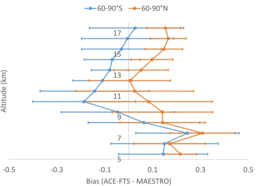
the bias between MAESTRO and ACE-FTS water vapour climatologies at both high latitude bands. An ACE-FTS high bias of∼10 % has been observed for the

extratrop-ical upper troposphere (40–80◦N and 40–80◦S, near 300 hPa) (Hegglin et al., 2013). While inconclusive, a general wet bias between 5 and 8 km is also suggested by lidar comparisons in the extratropics (Carleer et al., 2008; Moss et al., 2013). Accounting for

5

an upper tropospheric+10 % wet bias in ACE-FTS, MAESTRO and ACE-FTS agree within±20 % at all heights (5.5–17.5 km, in 1 km steps) in both hemispheres at high

latitudes.

At each height, the monthly climatology (e.g., Fig. 4) is subtracted from the time se-ries (e.g., Fig. 3) to give the absolute deseasonalized anomaly. Dividing the monthly

10

absolute anomaly by the monthly climatology gives the relative anomaly. Note that July and August 2011 were omitted from the MAESTRO southern high latitude climatology at 6.5–9.5 km (altitudes and months of Puyehue volcanic enhancement) since the AAO standard error determined by regression is improved in doing so (see Sect. 2.5). The same process is followed to generate anomalies of temperature, ozone, relative

hu-15

midity (RH), tropopause pressure, and tropopause height. The anomalies of relative humidity with respect to ice are based on pressure and temperature from the GEM assimilation system and an accurate saturation vapour pressure formulation (Murray, 1967). The latitude sampling anomaly is generated by calculating the average sam-pled latitude for each high-latitude band and then the mission-averaged latitude in each

20

high-latitude band is subtracted.

Note that, because conclusions below about the importance of the annular modes are reached based on water vapour anomalies and the fact the deseasonalization is sensor-specific (i.e. the time series observed by each instrument is deseasonalized using its own climatology), overall biases and seasonally-dependent biases are actually

25

(11)

ACPD

15, 22291–22329, 2015

C. E. Sioris et al.

Title Page

Tables Figures

◭ ◮

Back Close

Full Screen / Esc

Discussion

P

a

per

|

Discussion

P

a

per

|

Discussion

P

a

per

|

Discussion

P

a

per

|

2.5 Regression analysis

We use a multiple linear regression analysis to determine the contribution of the ap-propriate annular mode to the variability in deseasonalized water vapour at high lat-itudes as a function of altitude. The set of available basis functions include a lin-ear trend, the monthly AAO (Mo, 2000) and AO (Larson et al., 2005) indices (http:

5

//www.cpc.noaa.gov/products/precip/CWlink/) and a latitude sampling anomaly time series. This basis function is included to illustrate that sampling biases are minor even on a monthly time scale (using only the eight months which sample each high-latitude region). Note that the AO index is calculated following the method of Thompson and Wallace (2000).

10

When determining the response of water vapour to the AO, the AO index plus a con-stant are used, and the linear trend is included if it is significant at the 1σ_{level. When}

examining trend uncertainty reduction (Sect. 4.1), the regression uses a linear trend, plus a constant; the annular mode index term is included for trend determination if it improves the trend uncertainty without biasing the trend at the 1σ_level.

15

The types of biases that could aﬀect the analysis of water vapour variability are due to:

1. latitudinal sampling non-uniformity (Toohey et al., 2013),

2. interannual biases.

Regarding the non-uniform sampling of latitudes by the ACE orbit discussed in

20

Sect. 2.1, the correlation between monthly time series of average sampled latitude in the northern high-latitude region and the Arctic oscillation index is 0.19 and similarly the correlation between the monthly time series of average sampled latitude in the south-ern high-latitude region and the Antarctic oscillation index is 0.12. Given these very low correlations, ACE’s latitudinal sampling should have a negligible impact on any

25

(12)

func-ACPD

15, 22291–22329, 2015

C. E. Sioris et al.

Title Page

Tables Figures

◭ ◮

Back Close

Full Screen / Esc

Discussion

P

a

per

|

Discussion

P

a

per

|

Discussion

P

a

per

|

Discussion

P

a

per

|

tion. Toohey et al. (2013) estimated monthly mean sampling biases in the UTLS to be

≤10 % for the category of instruments that includes ACE-FTS (and MAESTRO). The

interannual biases are also<_{10 % given that Sect. 3.2 below shows that approximately}

half of the southern high-latitude water vapour seasonal anomaly (typically ±10 % in

amplitude) can be explained by interannual variability in the Antarctic oscillation (i.e.

5

real dynamical variability, not artificial instrument-related variability). Also, there are no known issues with either MAESTRO or ACE-FTS specific to a certain year. Further-more, the self-calibrating nature of solar occultation, combined with the wavelength stability of spectrometers (relative to filter photometers) minimize interannual bias for MAESTRO and ACE-FTS. For example, any variation in the optical (or quantum) eﬃ

-10

ciency of the instrument does not need to be calibrated as it does with an instrument measuring nadir radiance.

3 Results

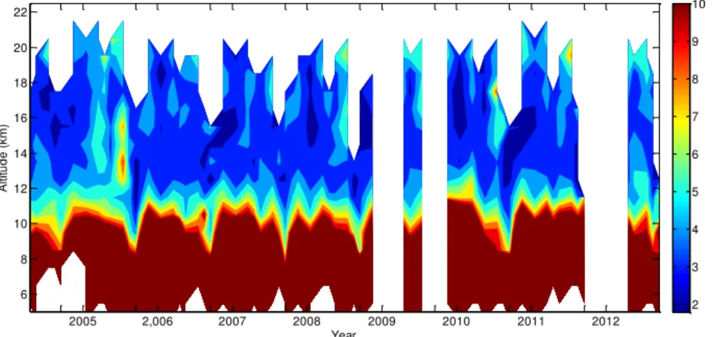
The MAESTRO water vapour record (Fig. 2) at southern high latitudes is similar to the records of contemporary limb sounders as shown in Fig. 13 of Hegglin et al. (2013).

15

The southern high-latitude time series has slightly less water in the UTLS in late winter than at northern high-latitudes (Fig. 3) due to the colder air temperatures.

3.1 Seasonal cycle

The dehydration in September that extends downward into the upper troposphere at southern high-latitudes (Fig. 4) is clearly observed by MAESTRO annually (Fig. 2).

20

(13)

ACPD

15, 22291–22329, 2015

C. E. Sioris et al.

Title Page

Tables Figures

◭ ◮

Back Close

Full Screen / Esc

Discussion

P

a

per

|

Discussion

P

a

per

|

Discussion

P

a

per

|

Discussion

P

a

per

|

the mid-troposphere, the driest month shifts closer to mid-winter (e.g. August). This is observed by both ACE instruments and by POAM III.

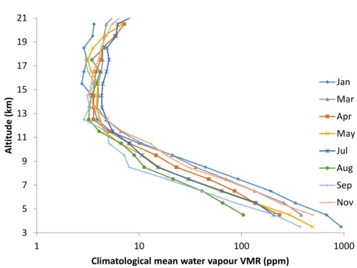
The vertical distribution of the lower stratospheric dehydration resembles that mea-sured from other solar occultation instruments: HALOE (Halogen Occultation Experi-ment) and POAM III in that the lowest water vapour mixing ratios occur at pressures

5

higher than 100 hPa (below 16 km) (Hegglin et al., 2013). The MAESTRO climatological mean mixing ratio for September exhibits a minimum at 12.5 km altitude with a value of 2.9 ppm (Fig. 4), which compares well with the September minimum values observed by other instruments (Hegglin et al., 2013). Also, the stratospheric monthly medians are reasonable with mixing ratios<_{7.5 ppm up to 22.5 km, the upper altitude limit of}

10

the climatology.

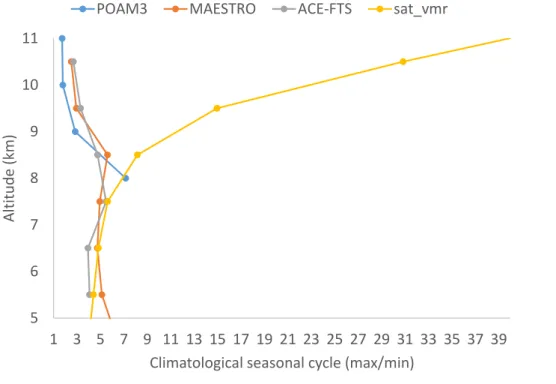
The variability in the UTWV at southern high latitudes on a monthly timescale is dominated by the seasonal cycle. The observed seasonal variation is a factor of∼5

at 8.5 km (Fig. 5). The seasonal cycle in water vapour is consistent with the ratio of maximum to minimum saturation vapour mixing ratio at 8.5 km of 4.6 (±1σrange: 3.9–

15

5.3), obtained for a typical year, namely 2010, using analysis temperatures and pres-sures from the GEM assimilation system, sampled at ACE measurement locations for January and August, the months corresponding to the maximum and minimum water vapour in ACE-FTS and POAM III data at 8.5 km. This is in stark contrast to weak (30 %) seasonal variations in lower stratospheric (13.5 km) monthly means, according

20

to MAESTRO observations. The large seasonal cycle amplitude in saturation vapour mixing ratio in the lower stratosphere is largely due to the extremely cold temperatures in September.

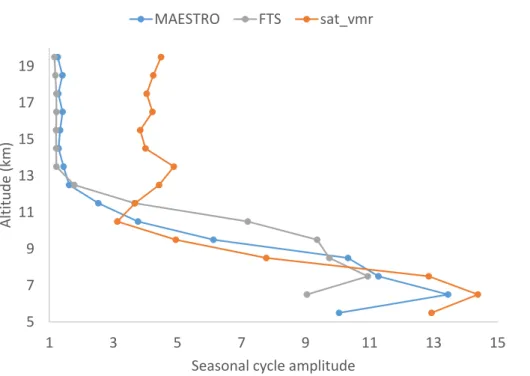
The stronger seasonal cycle at northern high-latitudes (e.g. at 5.5 km) is partly due to the non-uniform latitudinal sampling diﬀerences in the months of maximum and

mini-25

(14)

ACPD

15, 22291–22329, 2015

C. E. Sioris et al.

Title Page

Tables Figures

◭ ◮

Back Close

Full Screen / Esc

Discussion

P

a

per

|

Discussion

P

a

per

|

Discussion

P

a

per

|

Discussion

P

a

per

|

the seasonal cycle amplitude of the saturated VMR due to the isolation of this overly-ing atmospheric region from large sources of water vapour. Sioris et al. (2010) studied the seasonal cycle in the 60–70◦N band using an earlier version of the MAESTRO dataset. They incorrectly concluded that saturation vapour pressure changes could not explain the seasonal cycle assuming the seasonal cycle amplitude in temperature at

5

8.5 km was only 8 K (based on climatological subarctic winter and summer tempera-ture profiles). According to GEM temperatempera-ture analyses, the seasonal cycle amplitude is 18 K with a sharp peak in mid-summer (e.g. July) and generally suﬃcient to explain the seasonal variation and its vertical dependence in the upper troposphere (Fig. 6).

In spite of the large tropospheric seasonality at high latitudes, it is possible to

de-10

seasonalize the water vapour records from the ACE instruments and investigate the remaining sources of temporal variability, as shown next.

3.2 Antarctic oscillation

At 8.5 km, where the largest anti-correlations exist between MAESTRO water vapour at 8.5 km and the AAO index, it is observed that the anti-correlation is stronger on a

sea-15

sonal timescale (R=−0.53) rather than a monthly timescale. Stronger anti-correlation (R=−0.68) at the seasonal timescale is also found for ACE-FTS water vapour at

7.5±0.5 km, the altitude of its strongest anti-correlation with the AAO index. Thus,

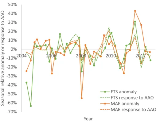
in Fig. 7, the MAESTRO and ACE-FTS seasonal median relative anomaly for 8.5±0.5 and 7.5±0.5 km, respectively, are presented. The use of medians is preferable for

de-20

tecting the AAO response in the troposphere where the water vapour mixing ratios are not normally distributed. The monthly medians are also less susceptible to outliers in the individual retrieved profiles. The large positive anomaly in 2011 is due to the most explosive eruption of a volcano in the last 24 years, namely Puyehue, and will be discussed in the forthcoming companion paper.

25

At 8.5 km, where the response of water vapour to AAO has the smallest relative un-certainty for both ACE-FTS and MAESTRO, the response ranges between +23 and

(15)

ACPD

15, 22291–22329, 2015

C. E. Sioris et al.

Title Page

Tables Figures

◭ ◮

Back Close

Full Screen / Esc

Discussion

P

a

per

|

Discussion

P

a

per

|

Discussion

P

a

per

|

Discussion

P

a

per

|

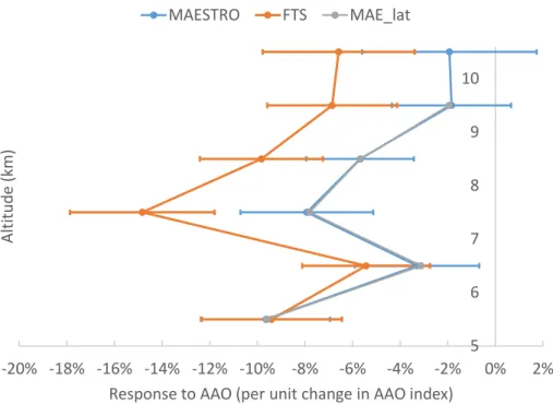
(2004–2012). The anomalies in the upper troposphere are highly correlated with each other (e.g.R=0.79 for MAESTRO absolute anomalies at 8.5 vs. 9.5 km on a monthly timescale). In the stratosphere (altitude ≥10 km), the response of MAESTRO water vapour to AAO is weak (not significant). Figure 8 illustrates the vertical profile of the AAO response. There is a strong vertical correlation between the water vapour

re-5

sponses to the AAO observed by the two instruments and the responses are statisti-cally significant (up to the 4σ _{level for ACE-FTS at 7.5 km) in the 5.5–8.5 km for both}

instruments indicating that the AAO affects water vapour throughout the upper tropo-sphere at southern high latitudes. The MAESTRO and ACE-FTS AAO fitting coeffi -cients are not different from 0 at the 1σ _{level at 10.5 and 11.5 km, respectively. Slight}

10

diﬀerences between the ACE instruments may relate to diﬀerences in their respec-tive fields of view (FOV). MAESTRO’s FOV is 1 km in the vertical direction, whereas ACE-FTS, because of its 3.7 km circular field of view at a tangent point 10 km above the ground, will see some contribution from the troposphere even when the FOV is centered 1.5 km above the tropopause. Given that the ACE-FTS field of view is

circu-15

lar, the full-width at half-maximum of the FOV is 3.2 km. Due to vertical oversampling of the FOV, the vertical resolution of the water vapour products from each ACE instrument is finer than the height of the FOV (see also Sioris et al., 2010). Nevertheless, diﬀ er-ences in vertical resolution between the ACE instruments will lead to a slight diﬀerence in terms of the peak altitude of the anti-correlation between the water vapour anomaly

20

and AAO. The impact of non-uniform latitudinal sampling is discussed in Sect. 3.3. As stated in Sect. 1, the AO is most active in the winter when the surface is coldest. Therefore less infrared (IR) radiation is emitted and trapped by AO-related increases in atmospheric water vapour. Over Antarctica, the AAO instead shows strength in late spring (Thompson and Wallace, 2000) at a time when there is increased IR radiation

25

(16)

ACPD

15, 22291–22329, 2015

C. E. Sioris et al.

Title Page

Tables Figures

◭ ◮

Back Close

Full Screen / Esc

Discussion

P

a

per

|

Discussion

P

a

per

|

Discussion

P

a

per

|

Discussion

P

a

per

|

of the atmosphere is assessed for November 2009 and November 2010, two months when the AAO was of opposite phase (see Appendix for details of the method). The cooling rate diﬀerences at the surface between these negative and positive phases of the AAO are trivial (<_{0.07 K) in late spring (November). The outgoing longwave flux is}

reduced by 0.7 W m−2in November 2009 relative to November 2010 due solely to

AAO-5

related upper tropospheric changes in water vapour. Scaling this change to the typical AAO fluctuation in all seasons (1979–2014), variations of 0.2 W m−2 in the outgoing longwave flux at the TOA are found, which are equal to the magnitude Li et al. (2014) found for the AO-related IR flux changes at TOA due to water vapour for the Arctic cold season. Note that Li et al. (2014) found the AO-related water vapour changes to be

10

much smaller than AO-related cloud changes.

3.3 Arctic oscillation

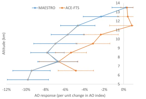
Figure 9 shows the altitude dependence of observed water vapour response to the Arctic oscillation using all eight months that sample the northern high-latitude region. There is a coherent and statistically significant response (up to the 4σ level for

MAE-15

STRO) to the AO observed by both instruments, with a general decrease through the upper troposphere and a vanishing response in the vicinity of the tropopause. Above 12 km, the response to the AO is insignificant at the 1σlevel. The magnitude of the re-sponse to the AO is also similar to the magnitude of the rere-sponse of UTWV at southern high latitudes to the Antarctic oscillation.

20

The spatiotemporal sampling of ACE (Bernath et al., 2005) is quite non-uniform on monthly time scales whereas on seasonal timescales the spatial coverage of the entire high-latitude region becomes more complete. This likely partly explains why a larger anti-correlation between southern high-latitude UTWV and the AAO index is found when a seasonal timestep is used. When the latitudinal sampling anomaly is used

25

(17)

rein-ACPD

15, 22291–22329, 2015

C. E. Sioris et al.

Title Page

Tables Figures

◭ ◮

Back Close

Full Screen / Esc

Discussion

P

a

per

|

Discussion

P

a

per

|

Discussion

P

a

per

|

Discussion

P

a

per

|

forcing the same finding for the response to the AAO (Fig. 8). Clearly, water vapour at high-latitudes is responding with high fidelity to the local annular mode.

Using the MAESTRO water vapour anomalies, a seasonal timestep and all seasons, 45 % of the variability is explained at 6.5±0.5 km, similar to the fraction obtained for

southern high latitudes.

5

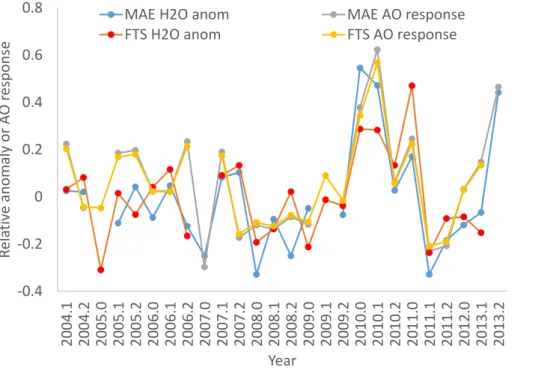
It is well known that the “active season” for the AO is winter (Thompson and Wal-lace, 2000). Figure 10 shows a water vapour anomaly time series for an altitude of 6.5 km, composed only of January, February and March (2004–2013). The winter-time anti-correlation between the ACE-FTS water vapour anomaly and the AO index peaks at 6.5 km withR=−0.57. MAESTRO shows a much stronger anti-correlation of

10

R=−0.80 at 6.5 and 5.5 km. A large negative AO event in March 2013 produced the

largest relative water vapour anomaly at 5.5 km (+70 %) over the MAESTRO record. March 2013 was not available below 8 km for ACE-FTS but at 8.5 and 9.5 km, ACE-FTS and MAESTRO both show the largest positive anomalies for any March in either north-ern high-latitude data record (+32 and+35 % at 8.5 km and+16 and+27 % at 9.5 km

15

for MAESTRO and ACE-FTS, respectively) and a vanishing enhancement at 10.5 km (above the monthly mean tropopause). A similarly large event in winter 2010, which was the largest negative AO event in the record (1950–2015), led to >50 and 30 % increases in northern high-latitude water vapour observed at 7.5 km in January and February 2010, respectively, with agreement between MAESTRO and ACE-FTS.

Jan-20

uary 2010 has the largest anomaly at 7.5 km in any month (considering all seasons) of the northern high-latitude data records of MAESTRO and ACE-FTS. Steinbrecht et al. (2011) used a multiple linear regression analysis to demonstrate a significant in-crease in total column ozone (+8 Dobson units) in the winter of 2010 that was attributed to the same historically strong negative phase of the Arctic oscillation.

(18)

ACPD

15, 22291–22329, 2015

C. E. Sioris et al.

Title Page

Tables Figures

◭ ◮

Back Close

Full Screen / Esc

Discussion

P

a

per

|

Discussion

P

a

per

|

Discussion

P

a

per

|

Discussion

P

a

per

|

4 Discussion and conclusions

Polar regions have a strong seasonal cycle in UTWV, driven by the seasonality of the local temperature. In the Arctic upper troposphere, condensation and precipitation play a minor role in governing the water vapour abundance on monthly timescales. Near the Arctic tropopause (250–350 mb), cloud fractions are<35 % (Treﬀeisen et al., 2007)

5

and MAESTRO monthly median relative humidity at 9.5 km is<_{70 % in all 63 months}

in which this instrument has observed the northern high-latitude region. However, dy-namical variability via the annular modes has been shown here to strongly aﬀect UTWV at high latitudes. Apart from the seasonal cycle, the Antarctic oscillation is a dominant mode of variability in upper tropospheric (∼8 km) water vapour at southern high

lati-10

tudes on a seasonal timescale and the Arctic oscillation explains most of the variability at wintertime UTWV in northern high latitudes.

4.1 Impact of fitting annular mode indices on decadal trends

In the most recent IPCC report, Hartmann et al. (2013) review the literature on trends in upper tropospheric water vapour observed from satellite instruments. Only one such

15

publication is cited, namely Shi and Bates (2011). This work uses HIRS data between 85◦N and 85◦S, but only trends at low latitudes (30◦N–30◦S) are discussed. While long-term trends in polar UTWV require continued measurements and investigation, including the AO index in the trend analysis improves trend uncertainties below 12 km over the MAESTRO record (e.g. by 16 % at 6.5 km) and reduces a statistically

insignif-20

icant (1σ) but consistent, positive bias in the decadal trend (2004–2013) that is found when the AO is excluded from the regression model. This bias stems from the two large negative events in the winters of 2010 and 2013 which lie near the end of the data record. The trend uncertainty reduction is 22 % upon inclusion of the Antarctic Oscillation Index into regression modelling of the linear trend in water vapour at 8.5 km

25

(19)

ACPD

15, 22291–22329, 2015

C. E. Sioris et al.

Title Page

Tables Figures

◭ ◮

Back Close

Full Screen / Esc

Discussion

P

a

per

|

Discussion

P

a

per

|

Discussion

P

a

per

|

Discussion

P

a

per

|

4.2 Proposed mechanisms

The amplitude of the response by water vapour to annular mode oscillations does not change significantly (1σ_{) whether upper tropospheric water vapour is binned vs.}

alti-tude or geopotential altialti-tude in either hemisphere at high latialti-tudes, indicating the insen-sitivity to the choice of vertical coordinate. This is important to note as the correlation

5

of other variables with the annular modes is explored in this section.

There is some observational evidence for two mechanisms that could explain how UTWV at high latitudes responds to the annular modes. The first is through annular-mode-related air temperature fluctuations, which impact UTWV by changing the satura-tion mixing ratio. For changes in saturasatura-tion mixing ratio to have an impact, there needs

10

to be an available supply of upper tropospheric water vapour. The second mechanism is through changes to the meridional flux itself (e.g. Devasthale et al., 2012; Thomp-son and Wallace, 2000), given the latitude gradient in water vapour between high and mid-latitudes at all upper tropospheric heights.

The anti-correlation of the AAO with anomalies in southern high-latitude

tempera-15

ture (from analyses of the GEM assimilation system) is also studied (Fig. 11). This anti-correlation is not strong (R=−0.34 at 5.5 km, and monotonically less correlated

with increasing height through the troposphere up to 10.5 km), indicating that southern high-latitude UTWV cannot be solely attributed to AAO-related temperature fluctuations but also requires an influx of high water vapour mixing ratios from mid-latitudes via the

20

second proposed mechanism. This argument is supported by the larger positive corre-lations of the AAO with ACE-FTS ozone anomalies (R=_{0.47 at 10.5 km, Fig. 11) which}

indicate that the AAO generally aﬀects the composition of the southern high-latitude up-per troposphere. For tropospheric ozone, the increasing correlation with height is likely due to the fact that latitudinal gradients in the mid-troposphere are weaker than for

25

(20)

ACPD

15, 22291–22329, 2015

C. E. Sioris et al.

Title Page

Tables Figures

◭ ◮

Back Close

Full Screen / Esc

Discussion

P

a

per

|

Discussion

P

a

per

|

Discussion

P

a

per

|

Discussion

P

a

per

|

At northern high latitudes, the strongest correlation of the AO with temperature in the 5.5 to 19.5 km is onlyR=−0.38 (at 6.5 km) and the correlation profile is very similar

in shape and magnitude to southern high latitudes (Fig. 11). Again, the anti-correlation vs. temperature is significantly weaker than between the AO and (MAESTRO) water vapour anomalies, which reach−0.56 at 6.5 km. However, the significant correlations

5

between AAO and ozone in the tropopause region seen in Fig. 11 for southern high-latitudes are not found in the north (Fig. 12). Thus, in the north, a combination of both mechanisms is required but the temperature-related mechanism appears to be more explanatory. This is explored further by studying the anti-correlation between relative humidity (RH) anomalies and the annular modes. At northern high-latitudes, a large

10

diﬀerence in anti-correlation with the AO exists between relative humidity and specific humidity (i.e. water vapour VMR) (Fig. 12). This implies that the temperature-related mechanism is largely responsible for the AO-related fluctuations in water vapour, with relative humidity maintained during these monthly fluctuations. However, at southern high-latitudes, the RH anomalies anti-correlate with the AAO almost as strongly as do

15

the water vapour anomalies, particularly near the tropopause (Fig. 11). This small diﬀ er-ence in correlation implies that the temperature-related mechanism is less explanatory at southern high latitudes and meridional flux of relative humidity can largely explain the water vapour anti-correlation with the AAO.

Thus, it appears that the major mechanism involved in the high anti-correlations of

20

the annular mode and water vapour anomalies could diﬀer between the two annular modes (i.e. between hemispheres). The dynamical mechanism may be more important at southern high latitudes in the upper troposphere where latitudinal gradients in water vapour and ozone (e.g. Liu et al., 2005, 2013) are likely larger than at northern high latitudes due to the isolated nature of the former region.

25

(21)

ACPD

15, 22291–22329, 2015

C. E. Sioris et al.

Title Page

Tables Figures

◭ ◮

Back Close

Full Screen / Esc

Discussion

P

a

per

|

Discussion

P

a

per

|

Discussion

P

a

per

|

Discussion

P

a

per

|

to the northern extratropical upper troposphere allows AO-related temperature fluc-tuations to eﬀectively increase UTWV. In the southern extratropics, the water vapour supply tends to be insuﬃcient above 8 km as is evident for from Fig. 5 which indicates that UTWV at southern high latitudes cannot match the local seasonal cycle ampli-tude of saturation VMR whereas Fig. 6 shows that in the northern high-latiampli-tude region,

5

UTWV tracks saturation VMR up to 10.5 km. Similarly, Fig. 12 shows that relative hu-midity anomalies below 7 km are much less correlated than UTWV anomalies with the AAO, implying that the temperature-related mechanism is generally limited to the altitude range with suﬃcient supply of humidity. This altitude range is quite diﬀerent between hemispheres, extending closer to the tropopause in the northern high-latitude

10

region. Furthermore, the lack of response in the stratosphere, e.g. at 13.5 km (Fig. 9), clearly above the maximum monthly tropopause height of 11.5 km, is due to the ineﬀ ec-tiveness of both mechanisms in spite of the large responses of both temperature and the meridional flux to the annular mode (Thompson and Wallace, 2000), peaking near 100 mb (∼16 km) for temperature, and between 200–300 mb (∼10 km) for the

merid-15

ional flux in both hemispheres. The temperature-related mechanism is ineﬀective in the stratosphere because temperature increases do not entail increases in water vapour in this dry region. The meridional flux mechanism becomes ineﬀective at 13.5 km be-cause the latitudinal water vapour gradients in the stratosphere are much weaker than in the troposphere.

20

We see no evidence in either high-latitude region of a third mechanism whereby the UTWV anomalies are simply explained by annular-mode-driven tropopause variations: the correlation between tropopause height or tropopause pressure anomalies and the relevant annular mode is not significant in either high-latitude region (−0.1< R <0.1). This is not surprising given that the magnitude of correlations of temperature and water

25

vapour with the annular modes diminish with increasing height toward the tropopause (e.g. Fig. 12).

(22)

ACPD

15, 22291–22329, 2015

C. E. Sioris et al.

Title Page

Tables Figures

◭ ◮

Back Close

Full Screen / Esc

Discussion

P

a

per

|

Discussion

P

a

per

|

Discussion

P

a

per

|

Discussion

P

a

per

|

Appendix: Cooling rate differences

Cooling rate vertical profiles are calculated using MODTRAN5.2 (e.g. Bernstein et al., 1996) assuming an Antarctic surface altitude of 2.5 km, subarctic summer temperature profile, free tropospheric aerosol extinction (visibility of 50 km) and two water vapour cases:

5

1. using MAESTRO climatological median water vapour between 6.5 and 9.5 km increased by the vertically-resolved water vapour response to AAO determined by multiple linear regression (with AAO and constant as the only predictors) for November 2009, when the AAO was in its negative phase (index of−1.92).

2. same as (1), except for November 2010, when AAO index was +1.52 (positive

10

phase).

Acknowledgements. The availability of the NOAA AAO index is appreciated. The ACE mission is supported primarily by the Canadian Space Agency. POAM III data were obtained from the NASA Langley Research Center Atmospheric Science Data Center. CES acknowledges Kaley Walker (University of Toronto) for her role in including MAESTRO in the Water Vapour

15

Assessment (WAVAS) 2, organized by SPARC (Stratosphere–Troposphere Processes and their Role in Climate). CES also acknowledges Frédéric Laliberté (Environment Canada) for his suggestion to analyze correlations of relative humidity anomalies with the annular modes and for guidance on the interpretation of those results.

References

20

Bates, J. J. and Jackson, D. L.: Trends in upper-tropospheric humidity, Geophys. Res. Lett., 28, 1695–1698, 2001.

Bernath, P. F., McElroy, C. T., Abrams, M. C., Boone, C. D., Butler, M., Camy-Peyret, C., Car-leer, M., Clerbaux, C., Coheur, P.-F., Colin, R., DeCola, P., DeMazière, M., Drummond, J. R., Dufour, D., Evans, W. F. J., Fast, H., Fussen, D., Gilbert, K., Jennings, D. E., Llewellyn, E. J.,

25

(23)

ACPD

15, 22291–22329, 2015

C. E. Sioris et al.

Title Page

Tables Figures

◭ ◮

Back Close

Full Screen / Esc

Discussion

P

a

per

|

Discussion

P

a

per

|

Discussion

P

a

per

|

Discussion

P

a

per

|

Semeniuk, K., Simon, P., Skelton, R., Sloan, J. J., Soucy, M.-A., Strong, K., Tremblay, P., Turnbull, D., Walker, K. A., Walkty, I., Wardle, D. A., Wehrle, V., Zander, R., and Zou, J.: At-mospheric Chemistry Experiment (ACE): mission overview, Geophys. Res. Lett., 32, L15S01, doi:10.1029/2005GL022386, 2005.

Bernstein, L. S., Berk, A., Acharya, P. K., Robertson, D. C., Anderson, G. P., Chetwynd, J. H.,

5

and Kimball, L. M.: Very narrow band model calculations of atmospheric fluxes and cooling rates, J. Atmos. Sci., 53, 2887–2904, 1996.

Boone, C. D., Walker, K. A., and Bernath, P. F.: Version 3 retrievals for the Atmospheric Chem-istry Experiment Fourier Transform Spectrometer (ACE-FTS). The Atmospheric ChemChem-istry Experiment ACE at 10: A Solar Occultation Anthology, edited by: Bernath, P. F., A. Deepak

10

Publishing, Hampton, Virginia, 2013.

Brewer, A. W.: Evidence for a world circulation provided by the measurements of helium and water vapour distribution in the stratosphere, Q. J. Roy. Meteor. Soc., 75, 351–363, 1949. Brown, L. R., Toth, R. A., and Dulick, M.: Empirical line parameters of H16₂ O near 0.94 µm:

positions, intensities and air-broadening coeﬃcients, J. Mol. Spectrosc., 212, 57–82, 2002.

15

Carleer, M. R., Boone, C. D., Walker, K. A., Bernath, P. F., Strong, K., Sica, R. J., Randall, C. E., Vömel, H., Kar, J., Höpfner, M., Milz, M., von Clarmann, T., Kivi, R., Valverde-Canossa, J., Sioris, C. E., Izawa, M. R. M., Dupuy, E., McElroy, C. T., Drummond, J. R., Nowlan, C. R., Zou, J., Nichitiu, F., Lossow, S., Urban, J., Murtagh, D., and Dufour, D. G.: Validation of water vapour profiles from the Atmospheric Chemistry Experiment (ACE), Atmos. Chem.

20

Phys. Discuss., 8, 4499–4559, doi:10.5194/acpd-8-4499-2008, 2008.

Dessler, A. E. and Sherwood, S. C.: A matter of humidity, Science, 323, 1020–1021, doi:10.1126/science.1171264, 2009.

Dessler, A. E., Schoeberl, M. R., Wang, T., Davis, S. M., and Rosenlof, K. H.: Stratospheric water vapor feedback, P. Natl. Acad. Sci. USA, 110, 8087–18091, 2013.

25

Devasthale, A., Tjernström, M., Caian, M., Thomas, M. A., Kahn, B. H., and Fetzer, E. J.: Influence of the Arctic Oscillation on the vertical distribution of clouds as observed by the A-Train constellation of satellites, Atmos. Chem. Phys., 12, 10535–10544, doi:10.5194/acp-12-10535-2012, 2012.

Gettelman, A., Weinstock, E. M., Fetzer, E. J., Irion, F. W., Eldering, A., Richard, E. C.,

30

(24)

ACPD

15, 22291–22329, 2015

C. E. Sioris et al.

Title Page

Tables Figures

◭ ◮

Back Close

Full Screen / Esc

Discussion

P

a

per

|

Discussion

P

a

per

|

Discussion

P

a

per

|

Discussion

P

a

per

|

Groves, D. G. and Francis, J. A.: Variability of the Arctic atmospheric moisture budget from TOVS satellite data, J. Geophys. Res., 107, 4785, doi:10.1029/2002JD002285, 2002. Hartmann, D. L., Klein Tank, A. M. G., Rusticucci, M., Alexander, L. V., Brönnimann, S.,

Charabi, Y., Dentener, F. J., Dlugokencky, E. J., Easterling, D. R., Kaplan, A., Soden, B. J., Thorne, P. W., Wild, M., and Zhai, P. M.: Observations: atmosphere and surface. in:

Cli-5

mate Change 2013: The Physical Science Basis. Contribution of Working Group I to the Fifth Assessment Report of the Intergovernmental Panel on Climate Change, edited by: Stocker, T. F., Qin, D., Plattner, G.-K., Tignor, M., Allen, S. K., Boschung, J., Nauels, A., Xia, Y., Bex, V., and Midgley, P. M., Cambridge University Press, Cambridge, UK and New York, NY, USA, 2013.

10

Hegglin, M. I., Tegtmeier, S., Anderson, J., Froidevaux, L., Fuller, R., Funke, B., Jones, A., Lin-genfelser, G., Lumpe, J., Pendlebury, D., Remsberg, E., Rozanov, A., Toohey, M., Urban, J., von Clarmann, T., Walker, K. A., Wang, R., and Weigel, K.: SPARC Data Initiative: com-parison of water vapor climatologies from international satellite limb sounders, J. Geophys. Res.-Atmos., 118, 11824–11846, doi:10.1002/jgrd.50752, 2013.

15

Herbin, H., Hurtmans, D., Clerbaux, C., Clarisse, L., and Coheur, P.-F.: H16₂ O and HDO mea-surements with IASI/MetOp, Atmos. Chem. Phys., 9, 9433–9447, doi:10.5194/acp-9-9433-2009, 2009.

Lacis, A. A., Schmidt, G. A., Rind, D., and Ruedy, R. A.: Atmospheric CO₂: principal control knob governing Earth’s temperature, Science, 330, 356–359, 2010.

20

Lambert, A., Read, W. G., Livesey, N. J., Santee, M. L., Manney, G. L., Froidevaux, L., Wu, D. L., Schwartz, M. J., Pumphrey, H. C., Jimenez, C., Nedoluha, G. E., Cofield, R. E., Cuddy, D. T., Daﬀ_{er, W. H., Drouin, B. J., Fuller, R. A., Jarnot, R. F., Knosp, B. W., Pickett, H. M.,}

Pe-run, V. S., Snyder, W. V., Stek, P. C., Thurstans, R. P., Wagner, P. A., Waters, J. W., Jucks, K. W., Toon, G. C., Stachnik, R. A., Bernath, P. F., Boone, C. D., Walker, K. A.,

Ur-25

ban, J., Murtagh, D., Elkins, J. W., and Atlas, E.: Validation of the Aura Microwave Limb Sounder middle atmosphere water vapor and nitrous oxide measurements, J. Geophys. Res., 112, D24S36, doi:10.1029/2007JD008724, 2007.

Laroche, S., Gauthier, P., St-James, J., and Morneau, J.: Implementation of a 3D variational data assimilation system at the Canadian Meteorological Centre. Part II: The regional

anal-30

(25)

ACPD

15, 22291–22329, 2015

C. E. Sioris et al.

Title Page

Tables Figures

◭ ◮

Back Close

Full Screen / Esc

Discussion

P

a

per

|

Discussion

P

a

per

|

Discussion

P

a

per

|

Discussion

P

a

per

|

Larson, J., Zhou, Y., and Higgins, R. W.: Characteristics of landfalling tropical cyclones in the United States and Mexico: climatology and interannual variability, J. Climate, 18, 1247–1262, 2005.

Li, Y., Thompson, D. W. J., Huang, Y., and Zhang, M.: Observed linkages between the northern annular mode/North Atlantic Oscillation, cloud incidence, and cloud radiative forcing,

Geo-5

phys. Res. Lett., 41, 1681–1688, doi:10.1002/2013GL059113, 2014.

Liu, G., Liu, J., Tarasick, D. W., Fioletov, V. E., Jin, J. J., Moeini, O., Liu, X., Sioris, C. E., and Os-man, M.: A global tropospheric ozone climatology from trajectory-mapped ozone soundings, Atmos. Chem. Phys., 13, 10659–10675, doi:10.5194/acp-13-10659-2013, 2013.

Liu, X., Chance, K., Sioris, C. E., Spurr, R. J. D., Kurosu, T. P., Martin, R. V., and

10

Newchurch, M. J.: Ozone profile and tropospheric ozone retrievals from the Global Ozone Monitoring Experiment: algorithm description and validation, J. Geophys. Res., 110, D20307, doi:10.1029/2005JD006240, 2005.

Lumpe, J., Bevilacqua, R., Randall, C., Nedoluha, G., Hoppel, K., Russell, J., Harvey, V. L., Schiller, C., Sen, B., Taha, G., Toon, G., and Vömel, H.: Validation of Polar Ozone and

15

Aerosol Measurement (POAM) III version 4 stratospheric water vapor, J. Geophys. Res., 111, D11301, doi:10.1029/2005JD006763, 2006.

McElroy, C. T., Nowlan, C. R., Drummond, J. R., Bernath, P. F., Barton, D. V., Dufour, D. G., Midwinter, C., Hall, R. B., Ogyu, A., Ullberg, A., Wardle, D. I., Kar, J., Zou, J., Nichitiu, F., Boone, C. D., Walker, K. A., and Rowlands, N.: The ACE-MAESTRO instrument on SCISAT:

20

description, performance, and preliminary results, Appl. Optics, 46, 4341–4356, 2007. Mo, K. C.: Relationships between low-frequency variability in the Southern Hemisphere and

sea surface temperature anomalies, J. Climate, 13, 3599–3610, 2000.

Moss, A., Sica, R. J., McCullough, E., Strawbridge, K., Walker, K., and Drummond, J.: Cal-ibration and validation of water vapour lidar measurements from Eureka, Nunavut, using

25

radiosondes and the Atmospheric Chemistry Experiment Fourier Transform Spectrometer, Atmos. Meas. Tech., 6, 741–749, doi:10.5194/amt-6-741-2013, 2013.

Murray, F. W.: On the computation of saturation vapor pressure, J. Appl. Meteorol., 6, 203–204, 1967.

Nedoluha, G. E., Bevilacqua, R. M., Hoppel, K. W., Lumpe, J. D., and Smit, H.: Polar Ozone and

30

(26)

ACPD

15, 22291–22329, 2015

C. E. Sioris et al.

Title Page

Tables Figures

◭ ◮

Back Close

Full Screen / Esc

Discussion

P

a

per

|

Discussion

P

a

per

|

Discussion

P

a

per

|

Discussion

P

a

per

|

Oman, L., Waugh, D. W., Pawson, S., Stolarski, R. S., and Nielsen, J. E.: Understanding the changes of stratospheric water vapor in coupled chemistry–climate model simulations, J. Atmos. Sci., 65, 3278–3291, 2008.

Randel, W. J., Moyer, E., Park, M., Jensen, E., Bernath, P., Walker, K., and Boone, C.: Global variations of HDO and HDO/H2O ratios in the upper troposphere and lower

strato-5

sphere derived from ACE-FTS satellite measurements, J. Geophys. Res., 117, D06303, doi:10.1029/2011JD016632, 2012.

Rothman, L. S., Gordon, I. E., Barbe, A., Benner, D. C., Bernath, P. F., Birk, M., Boudon, V., Brown, L. R., Campargue, A., Champion, J.-P., Chance, K., Coudert, L. H., Dana, V., Devi, V. M., Fally, S., Flaud, J.-M., Gamache, R. R., Goldman, A., Jacquemart, D., Kleiner, I.,

10

Lacome, N., Laﬀ_{erty, W. J., Mandin, J.-Y., Massie, S. T., Mikhailenko, S. N., Miller, C. E.,}

Moazzen-Ahmadi, N., Naumenko, O. V., Nikitin, A. V., Orphal, J., Perevalov, V. I., Perrin, A., Predoi-Cross, A., Rinsland, C. P., Rotger, M., Š_imeč_{ková, M., Smith, M. A. H., Sung, K.,}

Tashkun, S. A., Tennyson, J., Toth, R. A., Vandaele, A. C., Vander Auwera, J.: The HITRAN 2008 molecular spectroscopic database, J. Quant. Spectrosc. Ra., 110, 533–572, 2009.

15

Rydberg, B., Eriksson, P., Buehler, S. A., and Murtagh, D. P.: Non-Gaussian Bayesian retrieval of tropical upper tropospheric cloud ice and water vapour from Odin-SMR measurements, Atmos. Meas. Tech., 2, 621–637, doi:10.5194/amt-2-621-2009, 2009.

Shi, L. and Bates, J. J.: Three decades of intersatellite-calibrated High-Resolution Infrared Radiation Sounder upper tropospheric water vapor, J. Geophys. Res., 116, D04108,

20

doi:10.1029/2010JD014847, 2011.

Sioris, C. E., Zou, J., McElroy, C. T., McLinden, C. A, and Vömel, H.: High vertical resolution water vapour profiles in the upper troposphere and lower stratosphere retrieved from MAE-STRO solar occultation spectra, Adv. Space Res., 46, 642–650, 2010.

Soden, B. J. and Held, I. M.: An assessment of climate feedbacks in coupled ocean–

25

atmosphere models, J. Climate, 19, 3354–3360, doi:10.1175/JCLI3799.1, 2006.

Soden, B. J., Jackson, D. L., Ramaswamy, V., Schwarzkopf, M. D., and Huang, X.: The radiative signature of upper tropospheric moistening, Science, 310, 841–844, 2005.

Steinbrecht, W., Köhler, U., Claude, H., Weber, M., Burrows, J. P., and van der A, R. J.: Very high ozone columns at northern mid-latitudes in 2010, Geophys. Res. Lett., 38, L06803,

30

(27)

ACPD

15, 22291–22329, 2015

C. E. Sioris et al.

Title Page

Tables Figures

◭ ◮

Back Close

Full Screen / Esc

Discussion

P

a

per

|

Discussion

P

a

per

|

Discussion

P

a

per

|

Discussion

P

a

per

|

Su, H., Read, W. G., Jiang, J. H., Waters, J. W., Wu, D. L., and Fetzer, E. J.: Enhanced positive water vapor feedback associated with tropical deep convection: new evidence from Aura MLS, Geophys. Res. Lett., 33, L05709, doi:10.1029/2005GL025505, 2006.

Suen, J. Y., Fang, M. T., and Lubin, P. M.: Global distribution of water vapor and cloud cover sites for high-performance THz applications, IEEE Trans. Terahertz Sci. Technol., 4, 86–100,

5

2014.

Thompson, D. W. J. and Wallace, J. M.: Annular modes in the extratropical circulation. Part I: Month-to-month variability, J. Climate, 13, 1000–1016, 2000.

Toohey, M., Hegglin, M. I., Tegtmeier, S., Anderson, J., Añel, J. A., Bourassa, A., Brohede, S., Degenstein, D., Froidevaux, L., Fuller, R., Funke, B., Gille, J., Jones, A., Kasai, Y., Krüger, K.,

10

Kyrölä, E., Neu, J. L., Rozanov, A., Smith, L., Urban, J., von Clarmann, T., Walker, K. A., and Wang, R. H. J.: Characterizing sampling biases in the trace gas climatologies of the SPARC Data Initiative, J. Geophys. Res.-Atmos., 118, 11847–11862, doi:10.1002/jgrd.50874, 2013. Treﬀ_{eisen, R., Krejci, R., Ström, J., Engvall, A. C., Herber, A., and Thomason, L.: Humidity}

observations in the Arctic troposphere over Ny-Ålesund, Svalbard based on 15 years of

15

radiosonde data, Atmos. Chem. Phys., 7, 2721–2732, doi:10.5194/acp-7-2721-2007, 2007. Waymark, C., Walker, K. A., Boone, C. D., and Bernath, P. F.: ACE-FTS version 3.0 data set:

validation and data processing update, Ann. Geophys., 56, ag-6339, doi:10.4401/ag-6339, 2013.

Wiegele, A., Schneider, M., Hase, F., Barthlott, S., García, O. E., Sepúlveda, E., González, Y.,

20

Blumenstock, T., Raﬀalski, U., Gisi, M., and Kohlhepp, R.: The MUSICA MetOp/IASI H2O

andδ_{D products: characterisation and long-term comparison to NDACC/FTIR data, Atmos.}

Meas. Tech., 7, 2719–2732, doi:10.5194/amt-7-2719-2014, 2014.

Worden, J., Kulawik, S. S., Shephard, M. W., Clough, S. A., Worden, H., Bowman, K., and Gold-man, A.: Predicted errors of tropospheric emission spectrometer nadir retrievals from

spec-25

(28)

ACPD

15, 22291–22329, 2015

C. E. Sioris et al.

Title Page

Tables Figures

◭ ◮

Back Close

Full Screen / Esc

Discussion

P

a

per

|

Discussion

P

a

per

|

Discussion

P

a

per

|

Discussion

P

a

per

|

5 7 9 11 13 15 17

-0.5 -0.3 -0.1 0.1 0.3 0.5

Al

ti

tu

d

e

(km

)

Bias (ACE-FTS - MAESTRO)

60-90°S 60-90°N

(29)

ACPD

15, 22291–22329, 2015

C. E. Sioris et al.

Title Page

Tables Figures

◭ ◮

Back Close

Full Screen / Esc

Discussion

P

a

per

|

Discussion

P

a

per

|

Discussion

P

a

per

|

Discussion

P

a

per

|

Year

A

lt

it

u

d

e

(

k

m

)

2005 2,006 2007 2008 2009 2010 2011 2012 6

8 10 12 14 16 18 20 22

2 3 4 5 6 7 8 9 10

Figure 2. Time series of the MAESTRO monthly mean water vapour volume mixing ratio (VMR) vs. altitude (5.5–22.5 km) at southern high latitudes (60–90◦