Fluxes and concentrations of volatile organic compounds from a South-East Asian tropical rainforest

(1)

www.atmos-chem-phys.net/10/8391/2010/ doi:10.5194/acp-10-8391-2010

Chemistry

and Physics

Fluxes and concentrations of volatile organic compounds from a

South-East Asian tropical rainforest

B. Langford1, P. K. Misztal2,3, E. Nemitz2, B. Davison1, C. Helfter2, T. A. M. Pugh1, A. R. MacKenzie1, S. F. Lim*,**, and C. N. Hewitt1

1_{Lancaster Environment Centre, Lancaster University, LA1 4YQ, UK} 2_{Centre for Ecology & Hydrology, Bush Estate, Penicuik, EH26 0QB, UK} 3_{School of Chemistry, Edinburgh University, Edinburgh, EH9 3JJ, UK}

*_{formerly at: Malaysian Meteorological Department, Jalan Sultan, Petaling Jaya, Selangor Darul Ehsan, Malaysia} **_retired

Received: 20 April 2010 – Published in Atmos. Chem. Phys. Discuss.: 6 May 2010 Revised: 6 August 2010 – Accepted: 1 September 2010 – Published: 7 September 2010

Abstract. As part of the OP3 field study of rainforest atmospheric chemistry, above-canopy fluxes of isoprene, monoterpenes and oxygenated volatile organic compounds were made by virtual disjunct eddy covariance from a South-East Asian tropical rainforest in Malaysia. Approximately 500 hours of flux data were collected over 48 days in April– May and June–July 2008. Isoprene was the dominant non-methane hydrocarbon emitted from the forest, accounting for 80% (as carbon) of the measured emission of reactive carbon fluxes. Total monoterpene emissions accounted for 18% of the measured reactive carbon flux. There was no ev-idence for nocturnal monoterpene emissions and during the day their flux rate was dependent on both light and tempera-ture. The oxygenated compounds, including methanol, ace-tone and acetaldehyde, contributed less than 2% of the total measured reactive carbon flux. The sum of the VOC fluxes measured represents a 0.4% loss of daytime assimilated car-bon by the canopy, but atmospheric chemistry box modelling suggests that most (90%) of this reactive carbon is returned back to the canopy by wet and dry deposition following chemical transformation. The emission rates of isoprene and monoterpenes, normalised to 30◦C and 1000 µmol m−2s−1 PAR, were 1.6 mg m−2h−1 and 0.46 mg m−2h−1 respec-tively, which was 4 and 1.8 times lower respectively than the default value for tropical forests in the widely-used MEGAN

Correspondence to:B. Langford (b.langford1@lancaster.ac.uk)

model of biogenic VOC emissions. This highlights the need for more direct canopy-scale flux measurements of VOCs from the world’s tropical forests.

1 Introduction

(2)

8392 B. Langford et al.: Fluxes of VOCs above a SE Asian tropical rainforest studies have shown the aerosol yield from isoprene to be

small or negligible (Kroll et al., 2005, 2006; Kleindienst et al., 2006; Ng et al., 2008), yet the globally high emission rates of isoprene (500–750 Tg yr−1; Guenther et al., 2006) indicate that its contribution to organic aerosol may be sig-nificant (Zhang et al., 2007; Robinson et al., 2010), perhaps through the formation of water soluble compounds such as hydroxyhydroperoxides and epoxides (Paulot et al., 2009). However, Kiendler-Scharr et al. (2009) have demonstrated how isoprene emissions may actually suppress BSOA for-mation in a plant chamber study and thus its role remains unclear. Finally, in the presence of oxides of nitrogen, VOCs mediate in the formation of photochemical pollutants such as tropospheric ozone and peroxyacetyl nitrate (PAN) (e.g., Sillman, 1999; Hewitt et al., 2009). At high concentrations, ozone can be directly toxic with detrimental impacts on hu-man health, crops and forests (Fowler, 2008).

Despite the important roles played by VOCs in mediat-ing atmospheric composition and climate, relatively little is known about their emission rates from tropical forests. Cur-rent estimates suggest that these regions may account for up to half of all global BVOC emissions (Guenther et al., 2006), yet this estimate is based on a limited number of field studies. To date, the majority of these field observations have focused on tropical forests in Amazonia (Zimmerman et al., 1998; Helmig et al., 1998; Stefani et al., 2000; Rinne et al., 2002; Kuhn et al., 2007; Karl et al., 2007; Muller et al., 2008; Karl et al., 2009) and, to a lesser extent, regions of Africa (Klinger et al., 1998; Greenberg et al., 1999; Serca et al., 2001).

In current global biogenic VOC emission models such as the Model of Emissions of Gases and Aerosols from Nature (MEGAN G06) (Guenther et al., 2006), emissions of iso-prene from the world’s tropical forests are, in part, based on standardised emission rates calculated using measurements conducted in Amazonia. This assumes a degree of unifor-mity across all tropical forests, which has yet to be con-firmed by independent observations and which would be sur-prising, considering the variety of tree species in rainforests (Pitman et al., 1999), and the very substantial interspecies differences in BVOC emission rates amongst those species that have been measured (Guenther, 1997). The influence of seasonality, which has been shown to be significant in Ama-zonia (Kuhn et al., 2002; Muller et al., 2008; Barkley et al., 2009), but other important tropical forest regions have little or no seasonality in their climate (e.g. Borneo), again requir-ing model emission algorithms to be more region-specific. As well as providing improved estimates of natural BVOC emissions, region-specific measurements also benchmark the BVOC chemical climatology from which land-use change is causing deviations (Misztal et al., 2010a), with poten-tially serious implications for regional air quality (Hewitt et al., 2009). There is, therefore, an obvious need for more landscape-scale flux measurements, especially in SE Asia where to date no direct micrometeorological flux observa-tions have been made.

Here we present both direct canopy-scale concentration and flux measurements of a range of BVOCs (but not methane) above a tropical rainforest in SE Asia and com-pare the results to observations made in Amazonia and Africa (Sect. 3.2.1). Our findings are discussed in relation to the me-teorology and then used to optimise the light and temperature algorithms of the MEGAN model for the tropical forests of SE Asia (Sect. 3.2.2). Finally, the measured VOC fluxes are related to co-located measurements of CO2 exchange and a

canopy carbon budget is calculated.

2 Methods

2.1 Site description and setup

Measurements were made as part of the OP3 (Oxidant and Particle Photochemical Processes above a South-East Asian Rainforest) project (Hewitt et al., 2010a) at the Bukit Atur global atmosphere watch (GAW) station in the Danum Valley region of Sabah, Malaysia (4◦58′49.33′′N, 117◦50′39.05′′E, 426 m above mean sea level). The aims and objectives of the OP3 project are summarised by Hewitt et al. (2010a), who also give a detailed site description and overview of the mea-surements located at the GAW station. The flux footprint of the tower encompassed areas of both primary and selectively logged forest, with regions of both clear-felled-forest and oil palm plantations found some distance beyond, well outside the flux footprint. The selectively logged forest in the flux footprint was logged in 1988 and has since been rehabilitated by enrichment planting. Measurements were carried out over two separate four week periods with phase 1 (OP3-I) taking place during the months of April and May 2008 and phase 2 (OP3-III) occurring between June and July 2008. OP3-II consisted of measurements at a nearby oil palm plantation (Misztal et al., 2010a).

(3)

inspection and good agreement between CO2and H2O fluxes

measured with open and closed path sensors (sharing the same line) (Siong et al., 2010) confirmed that no condensa-tion occurred in the main inlet. Data from each sensor were logged onto a single laptop computer in combination with meteorological observations using a program written in Lab-VIEW 8.5 (National Instruments, Austin, Texas, USA).

Throughout the measurement period the PTR-MS operat-ing conditions were held constant to maintain anE/Nratio of approximately 140 Td, which represented the best compro-mise between the optimal detection limit for VOCs and the minimisation of the impact of high relative humidity (Hay-ward et al., 2002; Hewitt et al., 2003; Tani et al., 2004). Drift-tube pressure, temperature and voltage were typically main-tained at 0.165 kPa, 45◦C and 500 V respectively, which gave a primary ion count in the range 6 to 8×106ion counts per second (cps). The sensitivity (Snorm) of the PTR-MS for

each atomic mass unit (amu,m/z) was calculated at regular intervals using a gas standard (Apel-Riemer Environmental Inc.), which contained methanol, acetonitrile, acetaldehyde, acetone and isoprene at a nominal concentration of 1.0 ppmv each as well as limonene at 0.18 ppmv. Volume mixing ra-tios were calculated adopting the approach of Taipale et al. (2008), where the operating conditions of the PTR-MS are first standardised by normalizing the primary ion count to 1×106cps and accounting for the first water cluster: VMR=

_{I (}

RH+)norm

Snorm

(1) In this equation I(RH+)norm is the normalised count rate

(ncps) of an individualm/zwhich is calculated using Eq. (2):

I (RH+)norm=106

RHi

M21+M37−

RHzero

M21zero+M37zero

(2) Here RHi represents the ion count signal at mass Mi (cps), RHzerois the signal of the mass measured from the zero air

source,M21andM37are the counts of the primary (H18₃ O+) and reagent cluster ions H16₃ O+ H16₂ O+, respectively, while M21zeroand M37zeroare the primary and reagent cluster ions

when measuring from the zero air source.

Monoterpenes fragment in the drift tube to m/z 81 and 137 in a humidity dependent process, hence their sensitiv-ities were calculated as the sum of the two masses. For those compounds not contained in the gas mixture, empir-ical sensitivities were calculated based on the instrument-specific transmission characteristics. The transmission curve was calculated empirically in two stages, using two separate approaches. For the compounds in the lowerm/zrange, trans-mission coefficients were calculated using the approach of Taipale et al. (2008) , utilising the compounds contained in our on-site gas standard. For the higherm/zrange, where no suitable compound was present in our standard, the classi-cal transmission approach of Steinbacher et al. (2004) was adopted using a range of liquid standards. These standards

included the higher m/z compounds xylene (m/z 107) and camphor (m/z153) and the resulting transmission response was compared with the former approach to yield empirical sensitivities for the higherm/z’s. Calculating transmission coefficients empirically undoubtedly increases the level of uncertainty of the volume mixing ratios (vmrs), but this level varies depending upon the approach adopted. The approach of Taipale et al. (2008) is thought to lead to vmrs with an as-sociated uncertainty of±30% (e.g. Misztal et al. (2010b)), whereas vmrs calculated using the Steinbacher et al. (2004) approach can vary by as much as±100%. With this in mind, empirically derived vmrs for the lowerm/zrange, e.g. acetic acid and MVK+MACR, have a lower level of uncertainty than those in the higherm/zrange e.g.m/z83 (hexanals) and m/z85 (EVK). The remaining compounds presented in this study were all contained within our gas mixture and there-fore sensitivities were calculated directly and the uncertainty much lower.

During OP3-I the multi-component gas standard was not available. Consequently only isoprene could be calibrated di-rectly, using a low mixing ratio gas standard (4.52 ppbv±5%) (see Lee et al., 2006, for details). Subsequent analysis of the two isoprene standards by GC-FID showed less than 2% difference. Calibration for all other compounds measured during the first campaign was based on the empirically de-rived instrument specific transmission curve (Steinbacher et al., 2004), relative to isoprene.

2.2 PTR-MS operation and flux calculations

(4)

8394 B. Langford et al.: Fluxes of VOCs above a SE Asian tropical rainforest VOCs is not possible with the PTR-MS instrument and

con-tributions from mass fragments or other compounds with the same integer amu cannot be ruled out. In Table 1 we therefore summarise both the measured masses and the com-pounds most likely to contribute at each mass, as well as formulae, dwell times, instrument sensitivities and detection limits.

In order to account for the sampling delay induced by the distance between inlet and instrument, and so synchro-nise the PTR-MS data with that collected by the ultrasonic anemometer, a cross-correlation function of vertical wind ve-locity (w′) and scalar concentration (χ′) was used with the peak value chosen automatically over a 25 s time window. This procedure was applied to each individualm/zmeasured by the PTR-MS. Following this synchronisation, each 25-min flux file was then subject to a quality assessment, as described by Langford et al. (2010). Briefly, a two dimen-sional coordinate rotation was applied. Data were rejected during periods of non-stationarity and when the friction ve-locity (u∗) fell below 0.15 m s−1. The latter criterion resulted

in the rejection of approximately 27% of the collected data, while those that passed these criteria were ranked as either high- or low-quality, based on the exact outcome of the sta-tionarity test. The precision of each individual flux measure-ment was calculated at the 99.7% confidence interval follow-ing the procedure outlined by Spirig et al. (2005). This value was then used as a proxy for the limit of detection of the flux system and data that fell below this value were discarded. Rejecting data below this threshold ensured that all flux data presented in this manuscript were significantly different from zero.

2.3 Validity of flux measurements and potential losses In order to assess the validity of measurements made, sev-eral analyses were undertaken. Firstly, the integral turbu-lent statistics of the vertical wind velocity were evaluated by comparison of the measured ratio of the standard deviation of vertical wind component to friction velocity (σw/u∗) with

values obtained using the model of Foken et al. (2004), which predictsσw/u∗for a set of ideal conditions.

Following the assessment criteria used in the FLUXNET program (Foken et al., 2004), over 90% of the collected data were rated category 6 or better (i.e., suitable for general use) and less than 1% of the data qualified for rejection with a rank of class 9. This suggests that the turbulence encountered at this site, although light, was sufficiently well developed for the precise and accurate determination of fluxes and that flux measurements at this high measurement height were not ad-versely influenced by the effects of wake turbulence gener-ated by the tower or surrounding topography (Helfter et al., 2010).

The vDEC flux system was evaluated to establish flux losses due to bandwidth limitation. High frequency flux losses encountered due to the response time of the PTR-MS,

which cannot resolve fluctuations in the sub∼0.5 s range, were estimated from Horst (1997) and found to be negli-gible, and typically <2%. In contrast, the low frequency flux losses, arising from insufficient averaging periods, were more significant, as shown by Fig. 1. Theyaxes in this fig-ure show sensible heat fluxes calculated using averaging pe-riods of increasing length from panels A (1 h) to D (2.5 h) during the OP3 campaign. Thexaxes show the same data but the averaging periods are compiled of individual 30 min data files matched together. A high pass filter was applied to each 30 min file which ensured fluctuations from eddies with a time period greater than 30 min could not contribute to the flux measurement (Moncrieff et al., 2004). The slope of the regression between the two sets of fluxes provides an estimate of the flux missed due to the use of a 30 min averag-ing period. The results show that eddies with a time period of between 30 and 90 min increase the flux of sensible heat (H) by∼15%, while eddies with a period of 150 min carried a further 6% of the flux. Assuming similarity and identical frequency behaviour between sensible heat and VOC fluxes, it is probable that VOC fluxes measured at the GAW site us-ing 25 min averagus-ing periods will underestimate the true sur-face exchange by 15–20%. This relatively large contribution from low frequency eddies probably reflects our high mea-surement location and the values we report here are of a sim-ilar magnitude to those reported by Langford et al. (2010) for an analysis of data obtained from the comparibly high Tele-com Tower in central London. In contrast to this analysis, an investigation into the daytime energy budget closure at this site suggests closure to within 5% based on 30 min flux val-ues (Helfter et al., 2010). However, since the footprint of the net radiation measurements was not ideal, this closure may be slightly fortuitous.

(5)

Table 1. List of compounds measured during the OP3 campaigns, including their formula, dwell time, average sensitivity and detec-tion limit. Detection limits were calculated based on the signal to noise ratio of measured ion counts following Karl et al. (2003) (LOD=2×_σ_background_{/sensitivity).}

m/z Contributing compound(s) Formula Dwell time Average sensitivity Limit of Detection

[amu] [s] [ncps ppbv−1] [ppbv]

21 water isotope H18₂ O 0.1 s − − 33 methanol CH4O 0.5 s 11.6 1.2 37 water cluster (H₂O)2 0.1 s − − 42 acetonitrile C2H3N 0.5 s 19.6 − 45 acetaldehyde C2H4O 0.5 s 22.8 0.1 59 acetone C3H6O 0.5 s 25.2 0.1

propanal

61 acetic acid C2H4O2 0.5 s 26.5 0.09 69 isoprene C5H8 0.5 s 1.6 0.2

furan

methyl butenol fragment

71 methyl vinyl ketone C₄H₆O 0.5 s 27.1 0.07 methacrolein

81 monoterpene fragment − 0.5 s 4.0 0.04 83 hexanal fragment − _{0.5 s} _30.3 _0.04

cis−3−hexenol fragment

85 ethyl vinyl ketone C₅H₈O 0.5 s 30.3 0.06 137 monoterpenes C10H16 0.5 s 3.7 0.04 149 estragole C₁₀H₁₂O 0.5 s − − 205 sesquiterpenes C15H24 0.5 s − −

Figure 2 showsλEmeasured by PTR-MS and open-path IRGA over an 11-day period. Measured fluxes agree rea-sonably well (R2=0.56, p=<0.0001), but on average PTR-MS fluxes are lower, suggesting a typical flux loss of around

<17%. This flux loss is much larger than direct compar-isons between open and closed path IRGAλEfluxes, which showed just a 1% underestimation, again resulting from the long sample line (R2=0.93,p=<0.0001,y=0.9916x–0.9632). It should be noted that the PTR-MSλEfluxes are in fact sam-pled disjunctly, which, when cousam-pled with the indirect cali-bration against the closed-path IRGA may account for the larger disparity between the measurement systems.

The high measurement location of 75 m atop a hill also in-troduces the potential for flux divergence for the more reac-tive compounds such as isoprene, caused by changes in both convective mixing and isoprene chemistry across the day. We therefore estimated the effect of both isoprene chemistry and transport on the measurements made at our site.

In order to approximate the time taken between isoprene emission and detection by our measurement system, we esti-mated the mixing time to our measurement location using the convective velocity timescale (τmix), calculated as a function

of time of day.

τmix=

z w∗

(3)

wherezis the measurement height which was between 100 and 150 m above the average canopy top, here we use an ar-bitrary value of 125 m andw∗is equal to:

w∗= _gz

Tv

FH

1₃

(4) where,gis acceleration due to gravity (9.81 m s−2),Tvis po-tential temperature, andFH is the kinematic heat flux. The isoprene lifetime (τchem) was calculated using the isoprene

+ OH rate coefficient as a function of the ambient temper-ature (measured at 30 m) and the OH concentration which was directly measured at a height of 5 m at the base of the GAW tower (Whalley et al., 2010). Figure 3 shows τchem

(blue line) andτmix(red line) which follow a similar pattern,

with shorter mixing times and isoprene lifetimes occurring in the late morning and increasing steadily throughout the afternoon. The net effect of these two processes on our mea-surements of isoprene was calculated using the Damkohler¨ number (black line),

Da= τmix

τchem

(6)

8396 B. Langford et al.: Fluxes of VOCs above a SE Asian tropical rainforest

Fig. 1.An analysis of low frequency flux losses for sensible heat flux data(H) collected at the GAW site during the OP3 campaign. Solid line shows the best linear fit and dashed line represents the 1:1 line.

Fig. 2. (A)Latent heat fluxes measured at the GAW site during the period of 4–14 July by open path IRGA (LICOR – 7500) and PTR-MS. PTR-MS water vapour measurements recorded asm/z37 were calibrated against a closed path IRGA (LICOR – 7000) which sampled from the same 70 m sample line as the PTR-MS.(B)indicates the amount of flux lost due to attenuation along the long sample inlet and can be used to estimate a worst case scenario of VOC flux losses.

of isoprene. It should be noted that this calculation only con-siders the chemical loss after the compounds exit the canopy top and further chemical processing is likely to occur before emissions escape the canopy.

These analyses suggest that VOC fluxes measured at this site are underestimated due to a combination of insufficient

(7)

Fig. 3. The average boundary layer convective mixing velocity timescale (τmix) and isoprene lifetime (τchem) for the period 2– 21 July 2008 above a tropical rainforest. The Damkohler number¨ (black line) indicates the amount of isoprene that would be lost to chemical reaction before detection by our measurement system, which was located at 100–150 m above the forest canopy top. Be-cause the GAW tower is located on a hill it is not possible to give a more precise measurement height.

3 Results and discussion

3.1 Ambient BVOC mixing ratios

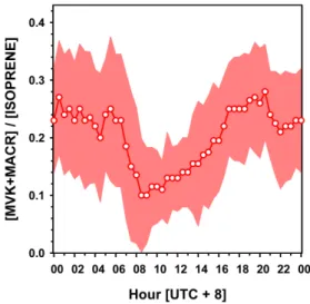
Figure 4 shows the average diurnal mixing ratios of the nine VOCs measured during the OP3 campaign and the results are summarised in Table 2a. During the daytime, mixing ratios for each compound were always above the calculated limit of detection, with the exception of methanol and m/z’s 83 and 85, which we tentatively ascribe to hexanal and/or cis-3-hexenol, and ethyl vinyl ketone (EVK), respectively. For methanol, instrument background counts were generally high but of a fairly constant amplitude. Consequently the detec-tion limit for methanol was relatively high despite the high sensitivity for this compound obtained in calibrations. Al-though our concentration measurements of methanol were always close to or below the detection limit, they are of a similar magnitude to measurements made by GC-FID during the campaign (Jones et al., 2010), hence their inclusion here. Although estragole (Misztal et al., 2010b) and sesquiterpenes were both targeted during the two campaigns, neither com-pound was detected by our system.

Isoprene was the second most abundant compound ob-served after methanol, accounting for approximately 30% (as compound) of the total measured species. Mixing ra-tios ranged between 0.17 and 3.4 ppbv with an average of 1.3 ppbv. Methacrolein (MACR) and methyl vinyl ketone (MVK), which are measured at the same atomic mass unit (amu) by the PTR-MS and consequently presented as the sum of the two (MACR+MVK), ranged between 0.05 and

0.67 ppbv, with an average value of 0.25 ppbv. Isoprene oxi-dation is the only known source of MACR and MVK; hence, the ratio of (MACR+MVK) to isoprene can provide an in-dication of the extent of isoprene oxidation. Average ra-tios of 0.16 and 0.22 were observed for the first and second campaigns, respectively. These findings are similar to ob-servations by Kesselmeier et al. (2002) who reported above-canopy ratios in Amazonia of 0.23 and 0.3 during the wet and dry seasons respectively. Similarly, Kuhn et al. (2007) reported a ratio of 0.3 for dry season measurements above Amazonia. Following the method of Karl et al. (2004), the average time taken between isoprene emission and detection by our system was estimated at between 16–22 min (based on the average midday [MVK+MACR]/[isoprene] ratio and an assumed atmospheric lifetime for isoprene of 100 min). Accordingly, isoprene mixing ratios were estimated to have originated from within a maximum footprint length of 2.8– 3.9 km (based on an average wind speed of 3 m s−1). This is slightly larger than the approximate footprint calculations reported by Helfter et al. (2010) for OP3 under unstable daytime conditions. This difference probably reflects the fact that isoprene emissions may take some time to exit the canopy and therefore undergo some chemical processing be-fore exiting the canopy.

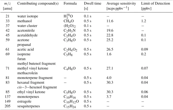
Figure 5 shows the [MVK+MACR]-to-[isoprene] ratio over the course of a typical day. The ratio has a distinct pat-tern, with a sharp decline observable at dawn as the nocturnal ratio decreased from 0.26 to 0.1 in the early morning. This relates to the response of the canopy to the increasing light and temperature which drives the isoprene emissions and a decrease in the transport time between canopy and the mea-surement height. As the isoprene emissions are transported away from the canopy they react to form more MVK+MACR which gradually accumulates in the boundary layer and thus the ratio increases steadily throughout the day before reach-ing a stable nocturnal maximum, when the isoprene emission and photochemistry shut off.

(8)

Fig. 4. Average diurnal profiles of VOC mixing ratios measured during the two intensive OP3 field campaigns which took place between 20 April–7 May (OP3-I) and 20 June and 20 July (OP3-III), 2008. Grey error bands show±1 standard deviation of averaged hourly values and dotted lines show the limit of detection (LOD=2×σbackground/sensitivity).

Fig. 5.Average diurnal profile of the MVK+MACR:isoprene ratio during OP3-III.

(9)

Table 2a.Summary of VOC mixing ratios (ppbv) measured during the two intensive OP3 campaigns.

Isoprene 6Monoterpene Methanol Acetaldehyde Acetone MVK+MACR Acetic acid Hexanal EVK

OP3 I (Wet)

Mean 1.1 0.24 1.2 0.36 0.91 0.23 0.40 0.05 0.05

Median 0.95 0.22 1.2 0.34 0.90 0.18 0.38 0.05 0.05

Percentiles

−95th 2.8 0.55 1.9 0.64 1.3 0.67 0.58 0.09 0.07

−5th 0.28 0.06 0.42 0.16 0.50 0.04 0.28 0.02 0.04

σ 0.80 0.15 0.46 0.14 0.22 0.20 0.09 0.02 0.01

n 746 744 746 751 704 745 755 703 751

OP3 III (Early Dry)

Mean 1.4 0.14 1.5 0.54 0.70 0.26 0.31 0.06 0.06

Median 1.1 0.10 1.4 0.52 0.68 0.19 0.30 0.06 0.06

Percentiles

−95th 3.6 0.44 2.7 0.84 0.99 0.67 0.43 0.09 0.10

−5th 0.12 0.05 0.48 0.31 0.45 0.05 0.20 0.03 0.03

σ 1.2 0.15 0.67 0.16 0.16 0.20 0.07 0.02 0.02

n 1269 1290 1252 1369 1364 1374 1372 1382 1378

OP3 All data

Mean 1.3 0.18 1.4 0.48 0.77 0.25 0.34 0.06 0.06

Median 1.0 0.15 1.3 0.47 0.75 0.19 0.33 0.06 0.05

Percentiles

−95th 3.4 0.48 2.5 0.78 1.1 0.67 0.50 0.09 0.09

−5th 0.17 0.02 0.46 0.22 0.46 0.05 0.22 0.03 0.03

σ 1.1 0.16 0.62 0.18 0.21 0.20 0.09 0.02 0.02

n 2015 2034 1999 2120 2068 2119 2127 2085 2129

Table 2b.Summary of VOC fluxes (mg m−2h−1) measured during the two intensive OP3 campaigns.

Isoprene 6Monoterpene Methanol Acetaldehyde Acetone MVK+MACR Acetic acid Hexanal EVK

OP3 I (Wet)

Mean 0.54 0.15 −0.02 0.01 0.007 −0.002 −0.005 0.004 0.004

Median 0.22 0.11 −0.05 0.02 0.009 −0.005 −0.006 0.006 0.005

Percentiles

−95th 2.2 0.62 0.30 0.11 0.12 0.08 0.05 0.05 0.05

−5th −0.12 −0.10 −0.34 −0.08 −0.09 −0.098 −0.061 −0.45 −0.035

σ 0.82 0.22 0.21 0.06 0.065 0.055 0.036 0.032 0.025

n 373 329 421 416 417 461 421 406 406

OP3 III (Early Dry)

Mean 1.2 0.29 −0.04 0.004 0.002 −0.002 −0.003 0.003 0.002

Median 0.76 0.21 −0.08 0.006 0.02 0.003 −0.01 0.005 0.004

Percentiles

−95th 4.0 0.92 0.51 0.13 0.12 0.091 0.058 0.034 0.032

−5th −0.38 −0.10 −0.60 −0.12 −0.081 −0.12 −0.059 −0.027 −0.03

σ 1.4 0.37 0.35 0.084 0.065 0.072 0.004 0.021 0.021

n 578 550 622 667 702 739 672 644 647

OP3 All data

Mean 0.93 0.24 −0.033 0.007 0.012 −0.002 −0.038 0.003 0.003

Median 0.46 0.16 −0.063 0.014 0.014 −0.002 −0.008 0.005 0.004

Percentiles

−95th 3.7 0.84 0.46 0.12 0.12 0.083 0.058 0.042 0.04

−5th −0.28 −0.11 −0.54 −0.11 −0.084 −0.11 −0.06 −0.035 −0.033

σ 1.3 0.33 0.3 0.073 0.065 0.066 0.037 0.026 0.023

(10)

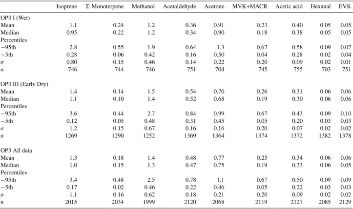
Fig. 6a. Summary of the meteorology and main VOC fluxes during the first intensive OP3 field campaign (OP3 – I) which took place during April and May, 2008. Wind speed and wind direction measurements were recorded by a senor (WXT-510 Weather Transmitter, Vaisala) situated at 75 m on the GAW tower. Temperature was recorded at 30 m by an aspirated thermocouple and sonic anemometer, PAR was measured from the roof of the GAW laboratory and sensible heat, friction velocity and VOC fluxes were all measured from the 75 m platform of the GAW tower. VOC flux data recorded during periods of low turbulence (u∗<0.15 m s−1) were rejected from the final analysis, but are shown here as grey circles.

3.2 Surface-layer VOC fluxes

3.2.1 Isoprene and monoterpene surface-layer fluxes

Figures 6a and 6b show measured isoprene and total monoterpene fluxes relative to the meteorological drivers light, temperature, wind speed/direction, frictional velocity and sensible heat flux, for both measurement phases and their statistics are summarised in Table 2b. During these periods, midday (10:00–14:00) temperature (at 30 m above ground) ranged between 23–28◦C, and photosynthetically active ra-diation (PAR) between 336–2027 µmol m−2s−1, whereas at night, temperatures fell to 22–24◦C. Sensible heat fluxes were positive during the day, ranging between 200 and 400 W m−2, with occasional troughs associated with con-vective cloud cover and rain events, as clearly seen on both 30 June and 5 July. Wind speed and friction velocities varied between 0.6–4.7 m s−1 and 0.06–0.52 m s−1 (5th–95th per-centiles), with particularly low values of both recorded at

night. Accordingly, VOC fluxes were generally only ob-served between 09:00 and 17:00 and not at night.

(11)

Fig. 6b. Summary of the meteorology and main VOC fluxes during the second intensive OP3 field campaign (OP3 – III) which took place during June and July, 2008. Measurement instrumentation as above. VOC flux data recorded during periods of low turbulence (u∗<0.15 m s−1) were rejected from the final analysis, but are shown here as grey circles.

profiles (1 m–32 m) of VOC mixing ratios within the for-est canopy. The targeted compounds included isoprene and monoterpenes and their source/sink distributions were de-rived using inverse Lagrangian modelling. These data did not show build up of either isoprene or monoterpenes inside the canopy during the night and indicate that dark emissions were negligible (Ryder et al., 2010). In contrast, early morn-ing emissions of both isoprene and monoterpenes which were driven by the rising sun and accumulated in the still shal-low nocturnal boundary layer, were occasionally observed as large spikes at around 08:00–09:00 during the break up of this stable air. The LIDAR measurements confirm that after sunrise the boundary layer quickly expanded. Therefore lit-tle of the daytime fluxes were lost due to de-coupling from the canopy.

Emissions of isoprene were the largest of all the mea-sured VOCs, with an average midday flux (10:00–14:00 LT) of 1.9 mg m−2h−1 for the entire 48-day period. This value represented approximately 80% (as carbon) of all mea-sured non-methane BVOC emissions from the forest canopy, with the remaining 20% accounted for by emissions of

(12)

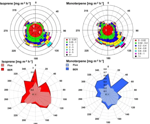
Fig. 7.Wind roses of isoprene and monoterpene fluxes (top) measured during the two OP3 campaigns. The bottom plots show the same raw flux data (light shading) and the base emission rate (solid shading) which is the raw flux normalised to standard conditions (30◦C (Canopy temperature), 1000 µmol m−2s−1) using the light and temperature algorithms from the MEGAN model (Guenther et al., 2006).

preparation for the coming dry season, resulting in an annual shutdown of isoprene emissions (Barkley et al., 2009). Simi-larly, M_{uller et al. (2008) have shown that isoprene emissions}¨ can be between 2–5 times lower during the wet season. Sea-sonality in Borneo is much less marked than in Amazonia; and our measurements showed no evidence of a similar pro-cess occurring at this site.

The average daytime ratio of monoterpene to isoprene fluxes was 0.23±_{0.3 (standard deviation) and remained} rela-tively constant throughout the day, including the period when early morning emissions were vented from the still shallow nocturnal boundary layer. This relative constancy suggests that nocturnal, light-independent emissions of monoterpenes are negligible at this site, which is consistent with Owen et al. (2002) and with the in-canopy profile measurements made by Ryder et al. (2010) who did not detect monoter-pene emissions from the darker understorey during the day or night-time build-ups inside the canopy. Guenther et al. (2008) summarise the monoterpene:isoprene emission ratios observed in other tropical forests, with values typically found to be∼0.15.

Polar plots of isoprene and monoterpene fluxes shown in Fig. 7 (top two panels), indicate that canopy emissions were spatially very heterogeneous, with observed fluxes strongly skewed towards the south-east. Analysis of po-lar plots for temperature and PAR shows a simipo-lar

south-east skew. This direction-dependent temperature effect was accounted for by normalising measured fluxes to give the base emission rate (BER; 30◦C (canopy temperature) and 1000 µmol m−2_s−1_{PAR). The resulting polar plots of BER}

(Fig. 7, bottom two panels) were less pronounced in the south east, but still showed considerable variability in emis-sion rates between wind sectors, with values ranging between 0.8 and 2.9 mg m−2h−1 for isoprene and between 0.2 and 0.7 mg m−2h−1for monoterpenes. Average BERs during the OP3 campaigns were 1.6 and 0.46 mg m−2h−1for isoprene and monoterpenes, respectively.

During the period between OP3-I and OP3-III Owen et al. (2010) made leaf-level measurements of isoprene and monoterpene emissions from the 25 most dominant over- and understorey tree species located within the flux footprint of the GAW tower. These species were sampled in situ and in triplicate using 3 controlled environment leaf cuvettes, which were set to 30◦C and a PAR value of either 500 or 1000 µmol m−2s−1, depending on whether the leaves were shaded or sunlit. The inflowing air was scrubbed to remove pre-existing VOCs whereas the CO2and humidity were

(13)

Table 3.Isoprene and monoterpene flux measurements from the world’s tropical forests and their typical ratios (monoterpene/isoprene). All values are in units of mg C m−2h−1. Where available, errors show±1 standard deviation.

Location Season Method Isoprene 6Monoterpene Ratio Reference

Borneo, SE Asia L Wet vDEC 0.48±0.72 0.13±0.19 0.27 Langford et al., this study Borneo, SE Asia E Dry vDEC 1.04±1.3 0.25±0.33 0.24 Langford et al., this study Malaysia, SE Asia Dry LL 1.1 − − Saito et al. (2008) Amazon, Brazil E Dry MB 2.7 0.24 0.23 Zimmerman et al. (1998) Amazon, Peru E Dry MLG 7.2 0.45 0.06 Helmig et al. (1998) Amazon, Brazil L Wet EC, REA 2.1 0.23 0.11 Rinne et al. (2002) Amazon, Brazil L Dry vDEC 7.3±2.7 1.5±1.1 0.21 Karl et al. (2007) Amazon, Brazil L Dry MLG 10.2±_3.5 _2.2±_0.7 _0.22 _{Karl et al. (2007)} Amazon, Brazil L Dry MLV 11.0±0.9 3.9±1.1 0.35 Karl et al. (2007) Amazon, Brazil E Dry REA 2.1±1.6 0.39±0.43 0.19 Kuhn et al. (2007) Amazon, Brazil E Dry SLG 3.4±3.6 0.38±0.58 0.11 Kuhn et al. (2007) Amazon, Brazil − REA 1.1 0.2 0.18 Stefani et al. (2000) Amazon, Brazil − BM 1.9 0.16 0.08 Greenberg et al. (2004) Amazon, Brazil − BM 4.7 0.20 0.04 Greenberg et al. (2004) Amazon, Brazil − _BM _8.6 _0.54 _0.06 _{Greenberg et al. (2004)} Amazon, Brazil Dry EC 0.4 – 1.5 − − Muller et al. (2008)¨ Amazon, Brazil Wet EC 0.1 – 0.3 − − Muller et al. (2008)¨ French Guyana, Dry CBL 6.1 − − Eerdekens et al. (2009) Suriname

Costa Rica Wet REA 2.2 − − Geron et al. (2002) Costa Rica Dry DEC 2.2 0.29 0.13 Karl et al. (2004) Congo, Africa − A−REA 0.9 − − Greenberg et al. (1999) Congo, Africa − LL 0.8−1 − − Klinger et al. (1998) Congo, Africa − _REA _0.46−_1.4 − − _{Serca et al. (2001)}

EC = Eddy covariance; vDEC = Virtual disjunct eddy covariance; DEC = Disjunct eddy covariance; (A)-REA = (Airborne) Relaxed eddy accumulation; SLG = Surface layer gradient; MB = Mass Budget; MLG = Mixed layer gradient; MLV = Mixed layer variance; LL = leaf level extrapolation; BM box = modelling; CBL = Convective boundary layer budgeting.

between 2000 and 2008, based on field-work in and around the Danum Valley area in 2000 and 2004, and from Dipte-rocarp rainforest species growing in the Yunnan Province, China, in 2003 and 2005. The database emission factors were used with vegetation survey data for different sample plots in the forest around the GAW tower for biomass weighted emis-sion extrapolations for the plots. Thus best bottom-up esti-mates of canopy emissions were obtained for different sam-ple plots with values ranging from 0.9 to 2.3 mg m−2h−1for isoprene and from 0.2 to 1.0 mg m−2h−1for total monoter-penes (Owen et al., 2010), which were in agreement with our direct canopy-scale flux measurements.

Although the extrapolated leaf-level measurements are on average larger than the measured fluxes, they are still well within the range of emission rates observed between wind sectors. The close agreement between canopy-scale fluxes and leaf-level measurements suggests that, although the tree species composition of the flux footprint is spatially hetero-geneous, up-scaling of leaf level measurements can still yield representative results for this area.

Table 3 summarises the isoprene and monoterpene fluxes measured during the OP3 campaigns relative to previous findings from Amazonia, Africa and South East Asia. Our measurements of isoprene compared very closely to leaf-level estimates made from a dipterocarp forest on mainland Malaysia (Saito et al., 2008) and to observations above re-gions of the Congo, but were at the extreme lower end of observations from Amazonia. In contrast, our measurements of total monoterpene fluxes are somewhat larger than those previously reported for other tropical forests.

3.2.2 Comparison of isoprene and monoterpene fluxes with modelled fluxes

(14)

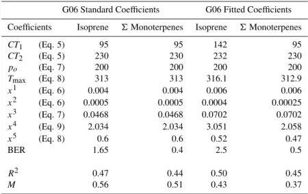
Table 4. Summary of the coefficients used to drive the MEGAN model. Standard coefficients are based upon studies of temperate plant species, whereas fitted coefficients relate to the measured flux data obtained during OP3-III over a tropical rainforest.

G06 Standard Coefficients G06 Fitted Coefficients

Coefficients Isoprene 6Monoterpenes Isoprene 6Monoterpenes

CT1 (Eq. 5) 95 95 142 95

CT₂ (Eq. 5) 230 230 232 230

po (Eq. 7) 200 200 200 200

Tmax (Eq. 8) 313 313 316.1 312.9

x1 (Eq. 6) 0.004 0.004 0.006 0.006 x2 (Eq. 6) 0.0005 0.0005 0.0004 0.00025 x3 (Eq. 7) 0.0468 0.0468 0.0702 0.0702 x4 (Eq. 9) 2.034 2.034 3.051 2.058 x5 (Eq. 8) 0.6 0.6 0.52 0.47

BER 1.65 0.4 2.5 0.5

R2 0.47 0.44 0.50 0.45

M 0.56 0.51 0.43 0.37

in the G06 algorithm were optimised for the emissions data reported in this paper by minimising the normalised mean square error (M) between observed and modelled data using a quasi-Newton Raphson iterative method (Microsoft Excel 2003, Microsoft Corporation, Redmond, WA, USA):

M= E0−Ep 2

E0·Ep

(6)

HereEois the observed emission,Epis the predicted

emis-sion and over bars denote mean values. The performance of the model is rated by the M score, which is a function of bias magnitude, bias variance and intensity of association (Guenther et al., 1993) and decreases with increasing model performance. In order to constrain the optimisation to envi-ronmentally realistic conditions, each coefficient was given a tolerance of±50%, with the exception of the temperature maximum (Tmax) which was restricted to±1% to avoid

unre-alistically high or low temperatures. Table 4 lists the standard coefficients presented by Guenther et al. (2006) and the new optimised coefficients based on the results of this study.

Model variables such as PAR and temperature (past and present) were supplied from the in situ measurements made at the GAW station. Before use, the ambient air tempera-ture measurements were first converted to give the canopy leaf temperatures required by the model using the resistance analogy described by Nemitz et al. (2009). Leaf tempera-tures during the afternoon were up to 2◦C higher than air temperature. Base emission rates describing isoprene and monoterpene emissions under constant (standard) conditions of temperature and PAR were inferred from the measured fluxes as described above. Our analysis assumes, as do all previous such analyses, that the BER is constant through-out the day. However, there are indications that BER varies

throughout the day and this finding is explored more fully elsewhere (Hewitt et al., 2010b). We therefore used the peak in the average diurnal cycle of BER measured at this site, which occured at around midday. Figure 8 shows the sim-ulated fluxes of isoprene (panel a) and monoterpenes (panel b) relative to the observed emissions over a 10-day period (2–12 July 2008).

(15)

Fig. 8.Isoprene and monoterpene fluxes (grey line) measured by the virtual disjunct eddy covariance technique during the OP3-III field campaign. The blue line shows the model output when configured using the standard G06 coefficients and the red line shows the same output generated with empirically fitted parameters. Both sets of parameters, including basal emission rates normalised to 30◦C and 1000 µmol m−2s−1are listed in Table 3.

Optimisation of the standard G06 coefficients resulted in new, site specific, light and temperature curves, which are shown in Fig. 9. For isoprene, the temperature response (γT),

shown in panel A, doubles the normalised emission rates at peak values compared with the standard G06 response. The shape, higher Tmax and increased emission rate of the

fit-ted response is consistent with laboratory measurements of tropical plant species (Ficus virgataandFicus microcarpa) made by Oku et al. (2008). In contrast, optimisation of the temperature response based on monoterpene fluxes showed no deviation from the standard G06 response. Panel B shows the light response (γP) of the fitted coefficients alongside the

standard G06 light response. The fitted response of isoprene and monoterpenes are very similar, with emission rates fol-lowing a steeper gradient at lower PAR values and saturating from 500 µmol m−2s−1of PAR onwards. This light response curve is very similar to those derived from laboratory mea-surements of oil palm (Wilkinson, 2006), a biofuel crop very common to the region, but not present within the GAW tower flux footprint, but differs significantly from sub-tropical tree species. For example, controlled environment measurements of isoprene emissions by Lerdau and Keller (1997) showed

Fig. 9. The temperature(A)and light(B)response of the G06 al-gorithm. Dashed lines show the G06 response using standard co-efficients which are based on temperate species only (in (A), the dashed line is directly below the blue line). Solid lines show the G06 response for isoprene (red) and monoterpenes (blue) using new coefficients which were obtained by fitting the algorithm response to measured fluxes above a tropical rainforest in Malaysian Bor-neo. In each response, past light and temperature values were set to: T24=297, T240=297, PAR24=360, PAR 240=375.

emission rates from sub-tropical tree species to increase with light intensity up to 2500 µmol m−2s−1 PAR. It should be noted that the optimised light and temperature curves pre-sented here are for canopy-scale emissions and therefore they should only be applied to canopies with a similar structure.

(16)

8406 B. Langford et al.: Fluxes of VOCs above a SE Asian tropical rainforest (2010a), Sect. 2.4), a parameter based on measurements

made over the Amazonian rainforest, to regions of Borneo would result in a>4 times overestimation of the emission rate. Similarly, applying the default total monoterpene emis-sion rate (0.8 mg m−2h−1) would result in an overestimation of>70%.

In addition to the activities described above, which utilise the leaf-level light and temperature algorithms of MEGAN, isoprene and monoterpene fluxes were also simulated us-ing the parameterised canopy environment emission algo-rithm (PCEEA), which is a simplified single-layer canopy-scale representation of the multi-layer model. This version of MEGAN uses a modified set of algorithms to describe the canopy-scale isoprene emission response to light and tem-perature. These algorithms are based on simulations from the detailed MEGAN canopy environment (CE) model for warm, broad leafed forests and account for factors such as light and temperature attenuation through the canopy. The PCEEA model is intended to reduce the computational ex-pense of running MEGAN in conjunction with a detailed CE model. When applied at the global-scale it can calculate iso-prene emissions to within 5% of the full MEGAN model, but may exceed 25% when applied at specific locations and times (Guenther et al., 2006).

Our application of the PCEEA model gave a poorer fit with the observations for both standard (R2=0.42, M=0.62) and fitted coefficients (R2=0.43, M=0.52) when com-pared to using the standard leaf-level G06 algorithms. Im-portantly, the PCEEA model does not utilise information on the previous light and temperature conditions (24–240 h). Therefore, it appears that at this site, it is more important to include details of the previous environmental conditions than to include information on the structure of the canopy and its attenuation of light and temperature, at least if this is done in this simplified way. However, it should be noted that using a detailed canopy environment model may well result in an improved fit, yet the implementation and validation of such a model would go well beyond the scope of the current paper.

Our findings highlight the need for more direct canopy-scale flux measurements of VOCs above the world’s tropical forests to allow for further evaluation and constraint of mod-els such as MEGAN.

3.2.3 Fluxes of other BVOCs

Fluxes of seven other BVOCs including methanol, acetone, acetaldehyde and acetic acid were measured during the two phases of the OP3 campaign; their average diurnal profiles are plotted alongside those of isoprene and monoterpenes in Fig. 10 with the results summarised in Table 2b. In addi-tion to the canopy emissions of isoprene and monoterpenes discussed above, positive fluxes of acetaldehyde, acetone, hexanal and/or cis-3-hexenol, and EVK, were also observed. Average emission fluxes of acetaldehyde and acetone were of a similar magnitude and range, but emissions of

ace-tone were larger during June and July relative to April and May, whereas acetaldehyde fluxes were slightly larger dur-ing April and May. Fluxes of hexanal and EVK were ap-proximately half that of acetone and acetaldehyde, averaging 20 µg m−2h−1, but mixing ratios of these two compounds were either very close to or below the limit of detection and therefore the fluxes of these compounds are not discussed further.

Previous studies over tropical forests have shown the bidi-rectional exchange of organic acids between canopy and at-mosphere (Kuhn et al., 2002; Karl et al., 2004). Our mea-surements are consistent with these findings, with deposition fluxes observed for acetic acid during morning and early af-ternoon as well as small emission fluxes at certain times. De-position velocities were in the range of 1–3 mm s−1, which is similar to those reported over the Amazonian rainforest by Kuhn et al. (2002) during the wet season. Correlations between instantaneous measurements of fluxes and ambient mixing ratios did not clearly show a compensation point as has been previously reported in leaf-level studies. However, it is likely that other sinks exist in the canopy (such as ad-sorption to leaf surfaces), which would affect the relationship between fluxes and concentrations. These findings should be treated with some caution as measurements of acetic acid by PTR-MS can be affected by memory effects in the inlet sys-tem and drift tube (de Gouw and Warneke, 2007).

Canopy profile measurements of methanol mixing ratios made by Ryder et al. (2010) showed elevated values close to the forest floor and their modelling of source/sink dis-tributions indicates the forest floor to act as a source for methanol at certain times. Previous studies have shown methanol to be emitted during the decomposition of leaf ma-terial (Fall, 2003). However, our canopy scale flux measure-ments showed periods of both emission and deposition, with small net deposition. Previous studies in Amazonia have also shown both positive and negative fluxes of methanol, but the net exchange has always been reported as posi-tive (Karl et al., 2004). The net deposition of methanol at this site, combined with its small deposition velocity, sug-gests that photo-oxidation is its primary source and results from the CiTTyCAT chemistry box model model indicate a methanol formation rate above the forest canopy of 1.7×105 molecules cm−3s−1, equivalent to about 0.6 ppbv day−1.

(17)

Fig. 10.Average diurnal profiles of VOC fluxes measured during the two intensive OP3 field campaigns which took place between 20 April– 7 May (OP3-I) and 20 June and 20 July (OP3-III), 2008. Greyed bands show±_{1 standard deviation of averaged hourly values.}

3.3 Net ecosystem exchange of carbon

Tropical forests assimilate carbon during the daytime and studies have shown that they currently act as a net carbon sink (Grace and Rayment, 2000). However, the carbon assimi-lated during the daytime is offset somewhat by the emission of VOCs from both the forest canopy and forest floor. We estimated this daytime offset by analysing total VOC emis-sions (all VOC measured during OP3; see Table 2b for list) with respect to concurrently measured CO2fluxes obtained

during the OP3-III campaign (20 June–20 July 2008). Fig-ure 11 shows the average diurnal profile of CO2fluxes and

total VOC exchange occurring above the forest canopy. In-tegrated CO2 fluxes yield a daytime (08:00–18:00) net

car-bon sink strength of 3120 mg C m−2d−1. Total VOC emis-sions, which had an integrated flux of 13.2 mg C m−2d−1 represented 0.4% of this (as carbon). The carbon offset from VOC fluxes above this SE Asian rainforest is lower than val-ues reported above an Amazonian forest (1.2−3.7 %; Kuhn et al., 2007; Karl et al., 2004), but this may be attributable to the limitations of the measurement system, which was de-coupled from the canopy at night (see above) and unable to resolve nocturnal CO2emissions due to respiration.

Conse-quently our estimates of net ecosystem exchange (NEE) are for daytime only and guaranteed to be an overestimate. For a more detailed discussion of CO2fluxes recorded during this

campaign see Siong et al. (2010).

(18)

Fig. 11. Averaged diurnal profiles of CO2and total VOC (sum of isoprene, monoterpenes, methanol, acetaldehyde, acetone, acetic acid, MVK+MACR, hexanal and EVK fluxes) fluxes measured above a SE Asian tropical rainforest during the period of 20 June– 20 July 2008. During the night time the measurements were de-coupled from the forest canopy and therefore data shown during that period are not representative of the exchange occuring at the canopy top. Error bars and green bands show±1 standard devia-tion of mean averaged values.

Isoprene was emitted following the diurnal cycle defined by the MEGAN algorithm (Guenther et al., 2006). The 24 h average emission rate was 6.88×1010molecules cm−2s−1 (0.28 mg m−2h−1). The only other emitted species was NO, at a constant rate of 6.53×109molecules cm−2s−1 (5.5 µg m−2h−1). A deposition velocity of 1.5 cm s−1 for MACR and MVK was adopted, following the findings of Pugh et al. (2010). Wet deposition (after Real et al., 2008, S-WET2 scheme) was also employed. The model does not include the formation of secondary organic aerosol, however the yields for isoprene are only a few percent (Hallquist et al., 2009). A carbon budget was calculated over the final four days of an eight-day model run, tracing the ultimate destina-tion of the carbon emitted as isoprene. The model run indi-cated that the bulk of the reactive carbon emitted from the canopy is rapidly returned to the canopy in the near vicin-ity of the point of emission through both wet (60%) and dry (27%) deposition processes. A small fraction (<4%) of the aldehydes, acids, nitrates and peroxides formed through pho-tochemical reactions persist to be either further oxidised or deposited on a longer timescale, but only 9% (0.04% of day-time NEE) of the emitted reactive carbon escapes the land-scape in the form of CO2. This fraction is somewhat lower

than the global average, which is thought to range between 23–55% (Goldstein and Galbally, 2007) and can be explained by the higher rates of wet and dry deposition found in the tropics.

4 Summary and conclusions

Direct canopy-scale measurements of VOC fluxes above a SE Asian tropical rainforest showed that isoprene was the dominant compound emitted, accounting for 80% (as car-bon) of the total measured reactive carbon fluxes. Typi-cal daytime fluxes ranged between 0.2 and 4.4 mg m−2h−1 (10:00–14:00; 5th and 95th percentiles), which, when nor-malised to standard conditions (30◦C; 1000 µmol m−2s−1 PAR), gave an average base emission rate of 1.6 mg m−2h−1. This value was found to be 4.1 times smaller than the default standard emission rate used in the MEGAN model for trop-ical forests. With the exception of BER, optimisation of the empirical coefficients describing the temperature and PAR response used within MEGAN did not significantly improve the fit between measured and modelled data, lending confi-dence to the global application of these coefficients.

Total monoterpenes accounted for 18% of the reactive carbon fluxes, ranging between −0.1 and 1.0 mg m−2h−1 (10:00–14:00; 5th and 95th percentiles) with an average base emission rate of 0.46 mg m−2h−1. This value was 70% lower than the standard emission rate for monoterpenes used in the MEGAN model for tropical forests. Combined with the evi-dence from in-canopy measurements, these data demonstrate that monoterpenes were not emitted at night and during the day they were found to be dependent on both light and tem-perature.

The fluxes of other VOCs including the OVOCs, methanol, acetaldehyde and acetone, accounted for <2% of the total reactive carbon flux. In total, the sum of the measured re-active carbon fluxes offset the daytime daytime assimilated carbon of the forest canopy by 0.4%, but atmospheric box modelling suggests that most (90%) of this reactive carbon is returned back to the canopy by wet and dry deposition fol-lowing chemical transformation.

Acknowledgements. BL sincerely thanks Liew Boon Seng and all those who cared for him at the Sabah Medical Centre. The OP3 project was funded by the UK Natural Environment Research Council (NE/D002117/1). We thank the Malaysian and Sabah Gov-ernments for their permission to conduct research in Malaysia; the Malaysian Meteorological Department for access to the Bukit Atur Global Atmosphere Watch station; Waidi Sinun of Yayasan Sabah and Glen Reynolds of the Royal Society’s South East Asian Rain Forest Research Programme for logistical support at the Danum Valley Research Station and the Royal Society research assistants Alexander Karolus, Johnny Larenus and Hadam Taman for logisti-cal support; Malcolm Possell, Annette Ryan, Kirsti Ashworth and Sue Owen for helpful discussion and the entire OP3 team for their individual and combined efforts. In particular, we acknowledge Gavin Phillips, Chiara Di Marco and Mhairi Coyle for help with the instrument setup on the GAW tower. This is paper 506 of the Royal Society’s South-East Asian Rainforest Research Programme.

(19)

References

Ammann, C., Brunner, A., Spirig, C., and Neftel, A.: Technical note: Water vapour concentration and flux measurements with PTR-MS, Atmos. Chem. Phys., 6, 4643–4651, doi:10.5194/acp-6-4643-2006, 2006.

Barkley, M. P., Palmer, P. I., De Smedt, I., Karl, T., Guenther, A., and Van Roozendael, M.: Regulated large-scale annual shut-down of Amazonian isoprene emissions?, Geophys. Res. Lett., 36, L04803, doi:10.1029/2008GL036843, 2009.

Claeys, M., Graham, B., Vas, G., Wang, W., Vermeylen, R., Pashyn-ska, V., Cafmeyer, J., Guyon, P., Andreae, M. O., Artaxo, P., and Maenhaut, W.: Formation of secondary organic aerosols through photooxidation of isoprene, Science, 303, 1173–1176, 2004. Davison, B., Taipale, R., Langford, B., Misztal, P., Fares, S.,

Mat-teucci, G., Loreto, F., Cape, J. N., Rinne, J., and Hewitt, C. N.: Concentrations and fluxes of biogenic volatile organic com-pounds above a Mediterranean macchia ecosystem in western Italy, Biogeosciences, 6, 1655–1670, doi:10.5194/bg-6-1655-2009, 2009.

de Gouw, J. and Warneke, C.: Measurements of volatile or-ganic compounds in the earths atmosphere using proton-transfer-reaction mass spectrometry, Mass Spectrom. Rev., 26, 223–257, 2007.

Donovan, R. G., Hope, E. S., Owen, S. M., Mackenzie, A. R., and Hewitt, C. N.: Development and Application of an Urban Tree Air Quality Score for Photochemical Pollution Episodes Using the Birmingham, United Kingdom, Area as a Case Study, Envi-ron. Sci. Technol., 39, 6730–6738, 2005.

Eerdekens, G., Ganzeveld, L., Vil`a-Guerau de Arellano, J., Kl¨upfel, T., Sinha, V., Yassaa, N., Williams, J., Harder, H., Kubistin, D., Martinez, M., and Lelieveld, J.: Flux estimates of isoprene, methanol and acetone from airborne PTR-MS measurements over the tropical rainforest during the GABRIEL 2005 campaign, Atmos. Chem. Phys., 9, 4207–4227, doi:10.5194/acp-9-4207-2009, 2009.

Evans, M. J., Shallcross, D. E., Law, K. S., Wild, J. O. F., Sim-monds, P. G., Spain, T. G., Berrisford, P., Methven, J., Lewis, A. C., McQuaid, J. B., Pilling, M. J., Bandy, B. J., Penkett, S. A., and Pyle, J. A.: Evaluation of a Langrangian box model us-ing field measurements from EASE (Eastern Atlantic Summer Experiment) 1996, Atmos. Environ., 34, 3843–3863, 2000. Fall, R.: Abundent oxygenates in the atmosphere: A biochemical

perspective, Chem. Rev., 103(12), 4941–4952, 2003.

Foken, T., Gckede, M., Mauder, M., Mahrt, L., Amiro, B., and Munger. W.: Post-field data quality control, in: Handbook of Micrometeorology: A guide for surface flux measurement and analysis, edited by: Lee, W. M. X. and Law, B., Dordrecht, Kluer Academic Publishers, 29, 181–203, 2004.

Fowler, D.: Ground-level ozone in the 21st century: future trends, impacts and policy implications, Royal Society, London, UK, 2008.

Geron, C., Guenther, A., Sharkey, T., and Arnts, R. R.: Temporal variability in basal isoprene emission factor, Tree Physiology, 20, 799–805, 2000.

Geron, C., Guenther, A., Greenberg, J., Loescher, H. W., Clark, D., and Baker, B.: Biogenic volatile organic compound emissions from a lowland tropical wet forest in costa rica, Atmos. Environ., 36, 3793–3802, 2002.

Goldstein, A. H. and Galbally, I. E.: Known and unexplored organic

constituents in the earth’s atmosphere, Environ. Sci. Technol., 41, 1514–1521, 2007.

Grace, J. and Rayment, M.: Respiration in the balance, Nature, 404, 819–820, doi:10.1038/35009170, 2000.

Granier, C., Petron, G., Muller, J. F., and Brasseur, G.: The impact of natural and anthropogenic hydrocarbons on the tropospheric budget of carbon monoxide, Atmos. Environ., 34, 5255–5270, 2000.

Greenberg, J. P., Guenther, A. B., Madronich, S., Baugh, W., Gi-noux, P., Druilhet, A., Delmas, R., and Delon, C.: Biogenic volatile organic compound emissions in central Africa during the experiment for the regional sources and sinks of oxidants (EX-PRESSO) biomass burning season, J. Geophys. Res.-Atmos., 104, 30659–30671, 1999.

Greenberg, J. P., Guenther, A. B., Petron, G., Wiedinmyer, C., Vega, O., Gatti, L. V., Tota, J., and Fisch, G.: Biogenic voc emissions from forested amazonian landscapes, Global Change Biol., 10, 651–662, 2004.

Guenther, A.: Seasonal and spatial variations in natural volatile or-ganic compound emissions, Ecol. Appl., 7, 34–45, 1997. Guenther, A., Karl, T., Harley, P., Wiedinmyer, C., Palmer, P. I.,

and Geron, C.: Estimates of global terrestrial isoprene emissions using MEGAN (Model of Emissions of Gases and Aerosols from Nature), Atmos. Chem. Phys., 6, 3181–3210, doi:10.5194/acp-6-3181-2006, 2006.

Guenther, A. B., Zimmerman, P. R., Harley, P. C., Monson, R. K., and Fall, R.: Isoprene and monoterpene emission rate variability – model evaluations and sensitivity analyses, J. Geophys. Res.-Atmos., 98, 12609–12617, 1993.

Guenther, A., Hewitt, C. N., Karl, T., Harley, P., and Reeves, C.: Biogenic VOC emissions from African, American and Asian tropical rainforests, Eos Trans. AGU, 89(53), Fall Meet. Suppl., Abstract A14C-04, 2008.

Hallquist, M., Wenger, J. C., Baltensperger, U., Rudich, Y., Simp-son, D., Claeys, M., Dommen, J., Donahue, N. M., George, C., Goldstein, A. H., Hamilton, J. F., Herrmann, H., Hoff-mann, T., Iinuma, Y., Jang, M., Jenkin, M. E., Jimenez, J. L., Kiendler-Scharr, A., Maenhaut, W., McFiggans, G., Mentel, Th. F., Monod, A., Pr´evˆot, A. S. H., Seinfeld, J. H., Surratt, J. D., Szmigielski, R., and Wildt, J.: The formation, properties and impact of secondary organic aerosol: current and emerging is-sues, Atmos. Chem. Phys., 9, 5155–5236, doi:10.5194/acp-9-5155-2009, 2009.

Hanson, D. T. and Sharkey, T. D.: Rate of acclimation of the capac-ity for isoprene emission in response to light and temperature, Plant Cell Environ., 24, 937–946, 2001.

Hayward, S., Hewitt, C. N., Sartin, J. H., and Owen, S. M.: Per-formance characteristics and applications of a proton transfer reaction-mass spectrometer for measuring volatile organic com-pounds in ambient air, Environ. Sci. Technol., 36, 1554–1560, 2002.

Helfter, C., Phillips, G. J., Coyle, M., Di Marco, C. F., Langford, B., Whitehead, J., Dorsey, J. R., Gallagher, M. W., Sei, E. Y., Fowler, D., and Nemitz, E.: Momentum and heat exchange above South East Asian rainforest in complex terrain, Atmos. Chem. Phys. Discuss., in preparation, 2010.

(20)

bio-8410 B. Langford et al.: Fluxes of VOCs above a SE Asian tropical rainforest genic nonmethane hydrocarbons within the planetary boundary

layer in the Peruvian Amazon, J. Geophys. Res.-Atmos., 103, 25519–25532, 1998.

Hewitt, C. N., Hayward, S., and Tani, A.: The application of proton transfer reaction-mass spectrometry (ptr-ms) to the monitoring and analysis of volatile organic compounds in the atmosphere, J. Environ. Monitoring, 5, 1–7, 2003.

Hewitt, C. N., MacKenzie, A. R., Di Carlo, P., Di Marco, C. F., Dorsey, J. R., Evans, M., Fowler, D., Gallagher, M. W., Hopkins, J. R., Jones, C. E., Langford, B., Lee, J. D., Lewis, A. C., Lim, S. F., McQuaid, J., Misztal, P., Moller, S. J., Monks, P. S., Ne-mitz, E., Oram, D. E., Owen, S. M., Phillips, G. J., Pugh, T. A. M., Pyle, J. A., Reeves, C. E., Ryder, J., Siong, J., Skiba, U., and Stewart, D. J.: Nitrogen management is essential to prevent trop-ical oil palm plantations from causing ground-level ozone pollu-tion, P. Natl. Acad. Sci. USA, 106, 18447–18451, 2009. Hewitt, C. N., Lee, J. D., MacKenzie, A. R., Barkley, M. P.,

Carslaw, N., Carver, G. D., Chappell, N. A., Coe, H., Col-lier, C., Commane, R., Davies, F., Davison, B., DiCarlo, P., Di Marco, C. F., Dorsey, J. R., Edwards, P. M., Evans, M. J., Fowler, D., Furneaux, K. L., Gallagher, M., Guenther, A., Heard, D. E., Helfter, C., Hopkins, J., Ingham, T., Irwin, M., Jones, C., Karunaharan, A., Langford, B., Lewis, A. C., Lim, S. F., MacDonald, S. M., Mahajan, A. S., Malpass, S., McFiggans, G., Mills, G., Misztal, P., Moller, S., Monks, P. S., Nemitz, E., Nicolas-Perea, V., Oetjen, H., Oram, D. E., Palmer, P. I., Phillips, G. J., Pike, R., Plane, J. M. C., Pugh, T., Pyle, J. A., Reeves, C. E., Robinson, N. H., Stewart, D., Stone, D., Whalley, L. K., and Yin, X.: Overview: oxidant and particle photochem-ical processes above a south-east Asian tropphotochem-ical rainforest (the OP3 project): introduction, rationale, location characteristics and tools, Atmos. Chem. Phys., 10, 169–199, doi:10.5194/acp-10-169-2010, 2010a.

Hewitt, C. N., Ashworth, K., Langford, B., MacKenzie, A. R., Mis-ztal, P. K., Nemitz, E., Owen, S. M., Possell, M., Pugh, T. A. M., Ryan, A. C., and Wild, O.: Circadian control reduces iso-prene emissions from forests and moderates ground-level ozone, in preparation, 2010b.

Horst, T. W.: A simple formula for attenuation of eddy fluxes mea-sured with first-order-response scalar sensors, Bound.-Lay. Me-teor., 82, 219–233, 1997.

Jenkin, M. E.: Chemical Mechanisms forming condensable ma-terial. AEA Technology Report, AEA/RAMP/20010010/002, 1996.

Jones, C. E., Hopkins, J. R., Langford, B., and Lewis, A. C.: Measurements of isoprene and speciated monoterpenes by GC-FID within a south-east Asian tropical rainforest, Atmos. Chem. Phys. Discuss., in preparation, 2010.

Karl, T. G., Spirig, C., Rinne, J., Stroud, C., Prevost, P., Green-berg, J., Fall, R., and Guenther, A.: Virtual disjunct eddy covari-ance measurements of organic compound fluxes from a subalpine forest using proton transfer reaction mass spectrometry, Atmos. Chem. Phys., 2, 279–291, doi:10.5194/acp-2-279-2002, 2002. Karl, T., Hansel, A., Mark, T., Lindinger, W., and Hoffmann, D.:

Trace gas monitoring at the Mauna Loa baseline observatory us-ing proton transfer reaction mass spectrometry, Int. J. Mass Spec-trom., 223–224, 527–538, 2003.

Karl, T., Potosnak, M., Guenther, A., Clark, D., Walker, J., Her-rick, J. D., and Geron, C.: Exchange processes of volatile organic

compounds above a tropical rain forest: Implications for model-ing tropospheric chemistry above dense vegetation, J. Geophys. Res.-Atmos., 109, D18306, doi:10.1029/2004JD004738, 2004. Karl, T., Guenther, A., Yokelson, R. J., Greenberg, J.,

Poto-snak, M., Blake, D. R., and Artaxo, P.: The tropical forest and fire emissions experiment: Emission, chemistry, and trans-port of biogenic volatile organic compounds in the lower atmo-sphere over Amazonia, J. Geophys. Res.-Atmos., 112, D18302, doi:10.1029/2007JD008539, 2007.

Karl, T., Guenther, A., Turnipseed, A., Tyndall, G., Artaxo, P., and Martin, S.: Rapid formation of isoprene photo-oxidation prod-ucts observed in Amazonia, Atmos. Chem. Phys., 9, 7753–7767, doi:10.5194/acp-9-7753-2009, 2009.

Kesselmeier, J., Kuhn, U., Rottenberger, S., Biesenthal, T., Wolf, A., Schebeske, G., Andreae, M. O., Ciccioli, P., Bran-caleoni, E., Frattoni, M., Oliva, S. T., Botelho, M. L., Silva, C. M. A., and Tavares, T. M.: Concentrations and species composition of atmospheric volatile organic compounds (VOCs) as observed during the wet and dry season in Ron-donia (Amazonia), J. Geophys. Res.-Atmos., 107(D20), 8053, doi:10.1029/2000JD000267, 2002.

Khare, P., Kumar, N., Kumari, K. M., and Srivastava, S. S.: At-mospheric formic and acetic acids: An overview, Rev. Geophys., 37(2), 227–248, 1999.

Kiendler-Scharr, A., Wildt, J., Dal Maso, M., Hohaus, T., Kleist, E., Mentel, T. F., Tillmann, R., Uerlings, R., Schurr, U., and Wah-ner, A.: New particle formation in forests inhibited by isoprene emissions, Nature, 461, 381–384, 2009.

Kleindienst, T. E., Edney, E. O., Lewandowski, M., Offenberg, J. H., and Jaoui, M.: Secondary organic carbon and aerosol yields from the irradiations of isoprene and alpha-pinene in the presence of NOxand SO2, Environ. Sci. Technol., 40, 3807–3812, 2006. Klinger, L. F., Greenberg, J., Guenther, A., Tyndall, G.,

Zimmer-man, P., M’Bangui, M., and Moutsambote, J. M.: Patterns in volatile organic compound emissions along a savanna-rainforest gradient in central Africa, J. Geophys. Res.-Atmos., 103, 1443– 1454, 1998.

Kroll, J. H., Ng, N. L., Murphy, S. M., Flagan, R. C., and Seinfeld, J. H.: Secondary organic aerosol formation from isoprene pho-tooxidation under high-NOx conditions, Geophys. Res. Lett., 32, L18808, doi:10.1029/2005GL023637, 2005.

Kroll, J. H., Ng, N. L., Murphy, S. M., Flagan, R. C., and Sein-feld, J. H.: Secondary organic aerosol formation from isoprene photooxidation, Environ. Sci. Technol., 40, 1869–1877, 2006. Kuhn, U., Rottenberger, S., Biesenthal, T., Ammann, C., Wolf, A.,

Schebeske, G., Oliva, S. T., Tavares, T. M., and Kesselmeier, J.: Exchange of short-chain monocarboxylic acids by vegetation at a remote tropical forest site in Amazonia, J. Geophys. Res.-Atmos., 107, 8069, doi:10.1029/2002JD000303, 2002.