ACPD
10, 18197–18234, 2010Influence of variations in isoprene
concentration
T. A. M. Pugh et al.
Title Page
Abstract Introduction
Conclusions References
Tables Figures
◭ ◮
◭ ◮
Back Close
Full Screen / Esc
Printer-friendly Version Interactive Discussion
Discussion
P
a
per
|
Dis
cussion
P
a
per
|
Discussion
P
a
per
|
Discussio
n
P
a
per
|
Atmos. Chem. Phys. Discuss., 10, 18197–18234, 2010 www.atmos-chem-phys-discuss.net/10/18197/2010/ doi:10.5194/acpd-10-18197-2010
© Author(s) 2010. CC Attribution 3.0 License.
Atmospheric Chemistry and Physics Discussions
This discussion paper is/has been under review for the journal Atmospheric Chemistry and Physics (ACP). Please refer to the corresponding final paper in ACP if available.
The influence of small-scale variations in
isoprene concentrations on atmospheric
chemistry over a tropical rainforest
T. A. M. Pugh1, A. R. MacKenzie1, B. Langford1, E. Nemitz2, P. K. Misztal2,3, and C. N. Hewitt1
1
Lancaster Environment Centre, Lancaster University, Lancaster, UK
2
Centre for Ecology and Hydrology, Edinburgh, UK
3
School of Chemistry, University of Edinburgh, Edinburgh, UK
Received: 16 April 2010 – Accepted: 21 April 2010 – Published: 30 July 2010
Correspondence to: T. A. M. Pugh (t.pugh@lancs.ac.uk)
ACPD
10, 18197–18234, 2010Influence of variations in isoprene
concentration
T. A. M. Pugh et al.
Title Page
Abstract Introduction
Conclusions References
Tables Figures
◭ ◮
◭ ◮
Back Close
Full Screen / Esc
Printer-friendly Version Interactive Discussion
Discussion
P
a
per
|
Dis
cussion
P
a
per
|
Discussion
P
a
per
|
Discussio
n
P
a
per
|
Abstract
Biogenic volatile organic compounds (BVOCs) such as isoprene constitute a large proportion of the global atmospheric oxidant sink. Their reactions in the atmosphere contribute to processes such as ozone production and secondary organic aerosol for-mation. However, over the tropical rainforest, where 50% of the global emissions of
5
BVOCs are believed to occur, atmospheric chemistry models have been unable to si-multaneously simulate the measured daytime concentration of isoprene and that of its principal oxidant, hydroxyl (OH). One reason for this model-measurement discrepancy may be incomplete mixing of isoprene within the convective boundary layer, leading to patchiness or segregation in isoprene and OH mixing ratios and average
concentra-10
tions that appear to be incompatible with each other. One way of capturing this effect in
models of atmospheric chemistry is to use a reduced effective rate constant for their
re-action. Recent studies comparing atmospheric chemistry global/box models with field
measurements have suggested that this effective rate reduction may be as large as
50%; which is at the upper limit of that calculated using large eddy simulation models.
15
To date there has only been one field campaign worldwide that has reported co-located measurements of isoprene and OH at the necessary temporal resolution to calculate
the segregation of these compounds. However many campaigns have recorded suffi
-ciently high resolution isoprene measurements to capture the small-scale fluctuations in its concentration. We use a box model of atmospheric chemistry, constrained by
20
the spectrum of isoprene concentrations measured, to estimate segregation intensity of isoprene and OH from high-frequency isoprene time series. The method
success-fully reproduces the only directly observed segregation. The effective rate constant
reduction for the reaction of isoprene and OH over a South-East Asian rainforest is
calculated to be typically <15%. This estimate is not sensitive to heterogeneities in
25
ACPD
10, 18197–18234, 2010Influence of variations in isoprene
concentration
T. A. M. Pugh et al.
Title Page
Abstract Introduction
Conclusions References
Tables Figures
◭ ◮
◭ ◮
Back Close
Full Screen / Esc
Printer-friendly Version Interactive Discussion
Discussion
P
a
per
|
Dis
cussion
P
a
per
|
Discussion
P
a
per
|
Discussio
n
P
a
per
|
model-measurement discrepancies for isoprene and OH above a rainforest.
1 Introduction
The volatile organic compound (VOC) isoprene (C5H8) is believed to account for 44%
of global biogenic emissions of VOCs (Guenther et al., 1995). The very high reac-tivity of isoprene with respect to common tropospheric oxidants makes its impact on
5
tropospheric chemistry, particularly in the planetary boundary layer (BL), very signifi-cant. Modelling studies have suggested that areas in which high emissions of isoprene occur, for instance the tropical rainforest or mid-latitude deciduous forests, should see suppression of hydroxyl radical (OH) concentrations in the boundary layer (Wang et al., 1998; Lawrence et al., 1999; Granier et al., 2000; Poisson et al., 2000; Lelieveld et al.,
10
2002; von Kuhlmann et al., 2004; J ¨ockel et al., 2006). This is of great consequence, as the OH radical is the primary sink for a large range of chemicals emitted into the atmosphere, including the greenhouse gas methane.
Over the past decade several measurement studies have noted much higher con-centrations of OH in areas of high isoprene concentration than has been predicted by
15
models of atmospheric chemistry (Tan et al., 2001; Carslaw et al., 2001; Ren et al., 2008; Lelieveld et al., 2008; Martinez et al., 2010; Hofzumahaus et al., 2009; Pugh et al., 2010). It has been proposed that the sources of OH in these high isoprene en-vironments may be underestimated and several suggestions for additional methods of OH formation have been put forward (Lelieveld et al., 2008; Hofzumahaus et al., 2009;
20
Peeters et al., 2009; Whalley et al., 2010). Whilst these methods are successful in
increasing modelled [OH]1in these regions to within the bounds of the measurements,
these increases in [OH] lead to faster oxidation, and hence lower concentrations, of isoprene. Butler et al. (2008) and Pugh et al. (2010) have shown that the increases in
1
ACPD
10, 18197–18234, 2010Influence of variations in isoprene
concentration
T. A. M. Pugh et al.
Title Page
Abstract Introduction
Conclusions References
Tables Figures
◭ ◮
◭ ◮
Back Close
Full Screen / Esc
Printer-friendly Version Interactive Discussion
Discussion
P
a
per
|
Dis
cussion
P
a
per
|
Discussion
P
a
per
|
Discussio
n
P
a
per
|
isoprene emission required to rectify this isoprene underestimation exceed the avail-able isoprene flux in these regions and furthermore lead to a re-suppression of [OH].
Butler et al. (2008) hypothesised that the reason for the discrepancy between mod-elled and measured isoprene and OH may lie with the rate of reaction between isoprene and OH used in chemical models. The rate of change of isoprene concentration with
5
respect to its reaction with OH can be represented by
∂hC5H8i
∂t =−kC5H8,OH(hOHihC5H8i+hOH
′
C5H8′i), (1)
where the angle brackets represent volume averages, and the primes represent devia-tions from the mean concentration. In a typical atmospheric chemistry model, concen-trations are assumed to be uniform within a box and the term containing the primes is
10
neglected. However studies with large eddy simulation (LES) models have shown that the contribution of the prime term can be substantial for atmospheric reactions where the timescale of the chemical reaction is of the same order as the mixing timescale (e.g. Schumann, 1989; Sykes et al., 1994; Krol et al., 2000; Patton et al., 2001;
Vin-uesa and Vil `a Guerau de Arellano, 2003). Using an intensity of segregation metric, S
15
(e.g. Krol et al., 2000), where
SC5H8,OH=
hOH′C5H8
′ i hOHihC5H8i
, (2)
this effect can be represented by a modified reaction rate constant,keff,
keff=kC5H8,OH(1+SC5H8,OH). (3)
A negative value of S implies that the two reactants are spatially anti-correlated,
20
whereas a positive value implies a positive correlation, and S=0 indicates a
homo-geneous distribution. In their idealised LES modelling study, Krol et al. (2000) found
that, under conditions of heterogeneous emissions, SVOC,OH=−0.294 was simulated
ACPD
10, 18197–18234, 2010Influence of variations in isoprene
concentration
T. A. M. Pugh et al.
Title Page
Abstract Introduction
Conclusions References
Tables Figures
◭ ◮
◭ ◮
Back Close
Full Screen / Esc
Printer-friendly Version Interactive Discussion
Discussion
P
a
per
|
Dis
cussion
P
a
per
|
Discussion
P
a
per
|
Discussio
n
P
a
per
|
and OH was 25% of that of the C5H8+OH reaction rate at 298 K (IUPAC, 2009).
Sim-ilarly, in the development of a parameterisation for segregation intensity, Vinuesa and
Vil `a Guerau de Arellano (2005) suggestSVOC,OH=−0.405, where the reactants react at
a rate similar to that of the C5H8+OH reaction rate at 298 K. Such segregation can
oc-cur for C5H8and OH because, due to the extremely rapid reaction rate between the two
5
compounds, [OH] rapidly approaches a steady state between its loss due to isoprene and its various production processes on a timescale of the order of one second (Ap-pendix A). Therefore if isoprene is not uniformly distributed throughout the model box, OH concentrations will also vary, with the lowest OH concentrations co-located with the highest isoprene concentrations, assuming other OH sinks are uniform. Isoprene
10
itself has a chemical lifetime in the boundary layer which is similar to typical turbulent mixing timescales (e.g. Butler et al., 2008; Pugh et al., 2010), while its flux into the BL is subject to heterogeneities likely influenced by the coupling of the canopy to the tur-bulent BL (e.g. Patton et al., 2001), the local dispersion of isoprene emitting plants, and variations in light and temperature. Therefore it is highly probable that heterogeneities
15
of isoprene concentration within the boundary layer will occur.
Based upon comparisons between measurements over the Amazonian rainfor-est and simulations using a global chemistry model, Butler et al. (2008) found
SC5H8,OH=−0.6 2
was required to reconcile measured and modelled concentrations if
the standard IUPAC rate constant for C5H8+OH is used. In a similar experiment, but
20
using a box model and measurements over a south-east Asian rainforest as part of the Oxidant Particle and Photochemical Processes (OP3) campaign, Pugh et al. (2010)
requiredSC5H8,OH=−0.5 to attain a good agreement between measurements and their
model. Considering that there is also a 20% uncertainty in the IUPAC rate constant, such values do not appear unreasonable in the context of the LES studies above.
25
Direct atmospheric measurements of segregation require co-located measurements
2
ACPD
10, 18197–18234, 2010Influence of variations in isoprene
concentration
T. A. M. Pugh et al.
Title Page
Abstract Introduction
Conclusions References
Tables Figures
◭ ◮
◭ ◮
Back Close
Full Screen / Esc
Printer-friendly Version Interactive Discussion
Discussion
P
a
per
|
Dis
cussion
P
a
per
|
Discussion
P
a
per
|
Discussio
n
P
a
per
|
of both species at a temporal resolution fast enough to resolve the smallest relevant
spatial scales. Butler et al. (2008) calculated a SC5H8,OH=−0.13 using aircraft
surements over the Guyanas; however at the speed of the aircraft the temporal mea-surement resolution resulted in a meamea-surement scale of the order of several hundred metres. Hence smaller scale segregation would have been missed. To date only one
5
study has measuredSC5H8,OHat a ground-based station, with Dlugi et al. (2010) finding
values ofSC5H8,OHas negative as−0.15 over a deciduous forest in Germany, although
their study is limited to a single day of measurements.
During OP3, high-temporal resolution measurements of [OH] co-located with those of isoprene were not available. Here we use high temporal resolution isoprene
concen-10
tration measurements (Langford et al., 2010) made over a south-east Asian rainforest as part of the OP3 campaign (Hewitt et al., 2010), in conjunction with a box model of atmospheric chemistry, to calculate [OH] and hence estimate the intensity of seg-regation of isoprene and OH in this region. First the measurements are described, followed by a description of the modelling approach used. Results are then presented
15
and discussed.
2 Measurements
Measurements of isoprene concentration were made using a proton-transfer reaction mass spectrometer (PTR-MS) during April/May 2008 at the Bukit Atur Global
Atmo-sphere Watch station (4◦58′59′′N, 117◦50′39′′E ). The station is located at an altitude
20
of 437 m a.m.s.l., on a small hill approximately 260 m above the valley floor and the surrounded by primary and secondary rainforest (Hewitt et al., 2010). On top of the hill stands a 100 m tall, open-pylon type tower which was instrumented with a sonic anemometer at 75 m and a low pressure (60 kPa) PTFE gas inlet tube (length: 85 m;
OD 12′′). For the purpose of turbulence calculations, these measurements are
consid-25
ered to be∼125 m above the forest canopy, taking into account that the measurement
ACPD
10, 18197–18234, 2010Influence of variations in isoprene
concentration
T. A. M. Pugh et al.
Title Page
Abstract Introduction
Conclusions References
Tables Figures
◭ ◮
◭ ◮
Back Close
Full Screen / Esc
Printer-friendly Version Interactive Discussion
Discussion
P
a
per
|
Dis
cussion
P
a
per
|
Discussion
P
a
per
|
Discussio
n
P
a
per
|
The PTR-MS was housed in an air-conditioned laboratory at the base of the tower
and sub-sampled from the inlet at a rate of 0.3 l min−1, via a short length of PTFE
tubing (18′′OD). The flow in the main inlet line was turbulent, minimising the dampening
of the VOC signal (Spirig et al., 2005). Individual compounds were sampled, iteratively,
proivding for each compound a disjunct time-series with a value every ∼7 s, that is
5
measured with an integration time of 0.5 s and an overall instrument response time of 1 s. These data are available for a continuous 25 min period out of every 30 min. The remaining 5 min were devoted to calibration techniques and scans of the mass spectrum. A complete description of these measurements and set-up can be found in Langford et al. (2010).
10
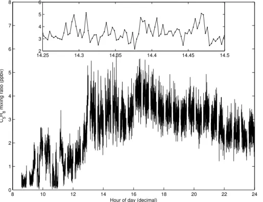
Figure 1 shows an example of isoprene concentration measurements for a single day (26 April 2008). Although the diurnal cycle in the measurements is clear, sub-stantial variation is seen around the mean. The inset indicates that these variations in isoprene concentration often have a magnitude similar to the mean isoprene con-centration. These fluctuations occur on a timescale of less than one minute. If they
15
are characteristic of the real atmosphere they indicate large inhomogeneities in the
isoprene distribution on length scales of<180 m, considering a wind speed<3 m s−1.
To test whether these concentration fluctuations are a real feature of the atmo-sphere, or are due to instrument noise, a statistical analysis was carried out. Hay-ward et al. (2002) showed that the instrument noise signal for the PTR-MS can be
20
well-approximated by a Gaussian distribution. They show that the standard deviation of noise varies with the signal strength can be reliably predicted by the noise statistic (NS):
NS=pc
c×δ
, (4)
wherecis the mean signal recorded by the PTR-MS in units of ion counts per second,
25
ACPD
10, 18197–18234, 2010Influence of variations in isoprene
concentration
T. A. M. Pugh et al.
Title Page
Abstract Introduction
Conclusions References
Tables Figures
◭ ◮
◭ ◮
Back Close
Full Screen / Esc
Printer-friendly Version Interactive Discussion
Discussion
P
a
per
|
Dis
cussion
P
a
per
|
Discussion
P
a
per
|
Discussio
n
P
a
per
|
The dwell time,δ, is the time spent scanning for each compound. For more information
on these terms the reader is referred to Hayward et al. (2002). As NS is analogous to standard deviation, if the rapid fluctuations in the measured isoprene concentration
are purely due to instrument noise, 4.4% of recorded values should fall outside±2NS
(Hayward et al., 2002).
5
Calculating NS for the isoprene concentration data collected between 10:00–
18:00 LT on 26 April 2008, using a 10 min running mean to calculatec, reveals that
10.5% of these data lie outside±2NS (3000 datapoints). This indicates that instrument
noise is highly unlikely to be responsible for all of the variation measured and shows that variations in isoprene concentration of this magnitude were present in the
atmo-10
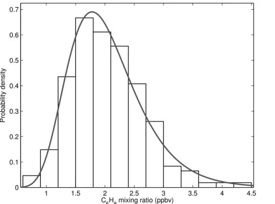
sphere during OP3. In addition, the distribution is close to log-normal (Fig. 2), which is representative of the statistical distribution of atmospheric concentrations, rather than random ion noise, which follows a Poisson distribution. Although it is not possible to
differentiate between the smaller variations and instrument noise, it is the large
fluctu-ations that will be of most importance in the analysis that follows.
15
3 Modelling
3.1 Approach
If a snapshot of the boundary layer is taken in time, a range of isoprene concentrations will be revealed in the spatial domain. Because isoprene is the dominant OH sink in the tropical forest environment, the variability in isoprene concentration induces
vari-20
ability in OH concentration. If isoprene is well mixed within the boundary layer, the variations in isoprene (and thus OH) concentrations will be small, and average
concen-trations are sufficient for calculations of chemistry. However, a boundary layer in which
isoprene is not well mixed will display a large standard deviation of concentrations for isoprene, which will induce a large variation in OH concentrations, resulting in a strong
25
ACPD
10, 18197–18234, 2010Influence of variations in isoprene
concentration
T. A. M. Pugh et al.
Title Page
Abstract Introduction
Conclusions References
Tables Figures
◭ ◮
◭ ◮
Back Close
Full Screen / Esc
Printer-friendly Version Interactive Discussion
Discussion
P
a
per
|
Dis
cussion
P
a
per
|
Discussion
P
a
per
|
Discussio
n
P
a
per
|
to describe the evolution of mixing air parcels of various concentrations in space. How-ever, here we argue that the variability in the OH concentration can be estimated on the basis of the variability of isoprene, if (a) the chemistry of OH in this tropical forest is
controlled mainly by isoprene, (b) isoprene is measured sufficiently fast to resolve the
fastest fluctuations that contribute to the co-variance with OH, and (c) the air advecting
5
past the measurement point is assumed to contain a range of isoprene concentrations representative of the boundary layer as a whole.
The ratio of turbulent timescale to chemical timescale is known as the Damk ¨ohler
ratio (Da). Turbulence and chemistry interact when Da is of the order of 1.
For Da≪1 turbulence controls the variability and for Da≫1 chemistry dominates
10
(Vil `a Guerau de Arellano et al., 1995). Under near-neutral conditions, the turbulent
dif-fusive time scale (τt) can be estimated as:
τt=κ(z−d)
σw2 , (5)
whered is the displacement height (defined as the effective height above the ground
surface; 20 m in this case),z is the measurement height (125 m),κ is the von Karmen
15
constant (0.38), andσw2 is the variance of the vertical wind component. Thus the typical
turbulence timescale,τt, is 200 s (corresponding to a length scale of≥800 m) between
10:00–16:00 LT, whilst the chemical timescale for the reaction between isoprene and
OH is fast, of the order one second (see Appendix A). ThusDa is of the order of 200
and turbulence is insufficiently fast to interact with the OH-isoprene chemistry, fulfilling
20
requirement (a).
The isoprene time-series represents 1 s average values approximately every 10 s. Assuming that Taylor’s frozen turbulence hypothesis (Powell and Elderkin, 1974) holds for reactive compounds, a measured isoprene concentration time-series with a tem-poral resolution of 1 s is transformed into a length scale, or spatial resolution, of 4 m
25
or less, when measured wind speeds are 4 m s−1 or less. Little is known about the
ACPD
10, 18197–18234, 2010Influence of variations in isoprene
concentration
T. A. M. Pugh et al.
Title Page
Abstract Introduction
Conclusions References
Tables Figures
◭ ◮
◭ ◮
Back Close
Full Screen / Esc
Printer-friendly Version Interactive Discussion
Discussion
P
a
per
|
Dis
cussion
P
a
per
|
Discussion
P
a
per
|
Discussio
n
P
a
per
|
isoprene and other chemical systems. In a study utilising a LES model, Vinuesa and Porte-Agel (2008) found that the sub-grid scale mixing term could be neglected when a
horizontal resolution of∼50 m or less was used. In this study, at the high measurement
height of 75 m,>90% of the variance and flux were estimated to be carried in eddies
slower than 1 Hz (Helfter et al., 2010; Langford et al., 2010) and it is likely that the
5
high-frequency contribution to the OH-isoprene co-variance is even smaller because of the damping induced by the fast chemistry. In addition, the close agreement found between the average of the 75-m isoprene measurements and aircraft measurements made in the boundary layer (Hewitt et al., 2009) gives confidence that the PTR-MS isoprene measurements at 75 m are representative of the boundary layer as a whole.
10
Thus, the isoprene measurement is though to be both representative and taken at a
sufficiently high temporal resolution for requirements (b) and (c) to be fufilled. Because
the isoprene measurement is non-continuous, it only provides a good statistical repre-sentation of the distribution of 1 s data points. However some of the information on the temporally organised structure in the variability gets lost. In the present model study
15
we assume that for each 1 s data point a stationary state between isoprene and OH
is obtained which is unaffected by the concentration history, since OH concentrations
re-equilibrate to a change in isoprene concentration on a timescale of the order of this
time (Appendix A).Therefore, given a sufficient time window,ts, a representative
sam-ple of the population of isoprene concentrations advected past the detector should be
20
obtained, and a histogram can be constructed showing the probability distribution of the measured isoprene concentration (Fig. 2).
By calculating the average sampled isoprene concentration and modelled OH
con-centration overts, estimates can be gained forhC5H8iandhOHi. Hence Eq. (2) eff
ec-tively becomes,
25
SC5H8,OH=
OH′C5H8′
OHC5H8
, (6)
ACPD
10, 18197–18234, 2010Influence of variations in isoprene
concentration
T. A. M. Pugh et al.
Title Page
Abstract Introduction
Conclusions References
Tables Figures
◭ ◮
◭ ◮
Back Close
Full Screen / Esc
Printer-friendly Version Interactive Discussion
Discussion
P
a
per
|
Dis
cussion
P
a
per
|
Discussion
P
a
per
|
Discussio
n
P
a
per
|
a time series measurement into a spatial scale of eddy size (evoking Taylor’s frozen turbulence hypothesis). Rather a set of discreet samples recorded in the time domain are used to represent the spatial variation of a population of those samples throughout
the boundary layer. An appropriate length fortsis discussed in Sect. 3.2.
We have already stated that the measured [C5H8] time-series is assumed to give a
5
representative sample of boundary layer [C5H8]. Therefore a corresponding
represen-tative sample of boundary layer [OH] can be calculated using
[OH]= POH−OLOH
kC5H8,OH[C5H8]
. (7)
WhereOLOHis the sum of all OH sinks other than C5H8, andPOHis the OH production
rate. As POH and OLOH are complex terms, they are most easily calculated using a
10
numerical chemistry model. By constraining a chemistry box model to the measured
[C5H8] time-series intervals, [OH] can be calculated. Note that this method does not
produce a continuous [OH] time-series, but rather a set of [OH] samples, which
corre-spond to the measured samples of [C5H8] at a given time. If the re-equilibration of OH
concentrations occurred over a longer time period than the isoprene sampling interval
15
then the model would not find the new steady-state [OH] before the next change in
[C5H8], and the model generated [OH] time-series would not be valid, given that no
in-formation exist on the isoprene concentration of 9 s after each 1 s sample. Appropriate
values for [OH] and [C5H8] are provided by taking running means over the time
win-dow,ts. So effectively a running sample of the population is being taken. This avoids
20
unnecessary and arbitary discretisation of the segregation signal and is similar to run-ning mean filtering in the calculation of surface exchange fluxes, i.e. co-variances of
concentration with wind components (McMillen, 1988). OH′and C5H8′ are then easily
calculated from the time series, and henceSC5H8,OHcan be calculated using Eq. (6).
An important consideration are the secondary oxidation products of isoprene, which
25
may be preferentially co-located with high isoprene concentrations, depending on the
life-ACPD
10, 18197–18234, 2010Influence of variations in isoprene
concentration
T. A. M. Pugh et al.
Title Page
Abstract Introduction
Conclusions References
Tables Figures
◭ ◮
◭ ◮
Back Close
Full Screen / Esc
Printer-friendly Version Interactive Discussion
Discussion
P
a
per
|
Dis
cussion
P
a
per
|
Discussion
P
a
per
|
Discussio
n
P
a
per
|
times of all secondary oxidation product of isoprene which may impact the OH sink
are much greater than the∼200 s turbulence timescale (Da≪1). Hence it is assumed
that the concentrations of secondary oxidation products of isoprene are not co-variant
with those of isoprene, and effectively consistute random noise in theSC5H8,OH signal.
Therefore it is better to assume a homogeneous mixture, averaging out the effects of
5
secondary species and limiting our conclusions to the segregation of isoprene and OH only. The use of the constrained box model in the manner described above implicitly mixes all species homogeneously across the modelled boundary layer if they have a lifetime longer than the sampling period.
Running a model constrained to measured concentrations is a typical approach for
10
studying chemical processes in the atmosphere and testing model chemical mech-anisms using both ground-based (e.g. Carslaw et al., 2001; Emmerson et al., 2005, 2007; Hofzumahaus et al., 2009; Kanaya et al., 2007, 2009) and aircraft-based (e.g. Ren et al., 2008; Kubistin et al., 2008) measurements. These studies typically use
measurements of VOCs, NOx, O3, CO and other intermediate/long-lived species, as
15
boundary conditions to attempt to calculate radical concentrations. However they all utilise measurements with a temporal resolution of greater than 1 min for the aircraft based measurements and in the region 5–15 min for the ground based measurements. All these studies are likely to miss much of the fine-scale segregation of species inves-tigated in this work.
20
3.2 Model setup
The CiTTyCAT box model of atmospheric chemistry (Wild et al., 1996; Evans et al., 2000; Emmerson et al., 2004; Donovan et al., 2005; Real et al., 2007, 2008; Hewitt et al., 2009; Pugh et al., 2010) is used to apply this approach to the OP3 measure-ments. The model is run for the 12 h of daylight between 06:00 and 18:00 LT, and
25
ACPD
10, 18197–18234, 2010Influence of variations in isoprene
concentration
T. A. M. Pugh et al.
Title Page
Abstract Introduction
Conclusions References
Tables Figures
◭ ◮
◭ ◮
Back Close
Full Screen / Esc
Printer-friendly Version Interactive Discussion
Discussion
P
a
per
|
Dis
cussion
P
a
per
|
Discussion
P
a
per
|
Discussio
n
P
a
per
|
gap. This is deemed acceptable as the characteristic spectrum of isoprene timescales is what is of interest in this analysis. If the 12 h data period contains gaps greater than 30 min, data for that day are discarded. In total eleven days of suitable data are available for analysis for the first OP3 campaign (OP3-1) (April–May 2008).
The model is integrated on a time step of 1 s, although the chemical solver itself
5
uses intermediate time steps of a variable size (Brown et al., 1989). As the model has previously been optimised for the OP3 scenario by Pugh et al. (2010), the set-up described in that paper is largely retained, with the model being fed campaign average
values of cloud cover (calculated using j(O1D) as a proxy) and temperature. Boundary
layer height is set to 800 m throughout the run. However it must be cautioned that
10
LIDAR measurements of boundary layer height (Pearson et al., 2010) indicate that the BL is well-mixed throughout this 800 m range only between the hours of 10:00– 18:00 LT. Therefore results before 10:00 LT will not be representative of the BL as a whole. Indeed the first hour must be discarded as spin-up time.
Finally, the length of the time window,ts, is of importance. When selectingtsit must
15
be considered what elements should be classified as segregation and at what time-scale variations start to reflect changing conditions (non-stationarities). For instance,
ifts=1 h, then variations in cloud cover and solar zenith angle may make a significant
contribution to the variation. However, cloud cover and solar zenith angle changes are typically uniform across the boundary layer and therefore do not contribute to the
20
spatial variation which is the subject of this work. In order to ensure that only
fac-tors such as canopy emission and BL turbulence dominate the variation, a shorterts
is required. To determine how short, the fast Fourier transform of measured j(O1D)
(which implicitly incorporates both cloud cover and solar zenith angle changes) is com-puted (not shown); this indicates little variation on timescales shorter than 10 minutes,
25
suggestingts=10 min would be sufficiently small to eliminate the effect of these lower
frequency variations. Conveniently the BL turnover timescale, as calculated by Pugh et al. (2010), is also close to 10 min, hence a time window of this length should be
ACPD
10, 18197–18234, 2010Influence of variations in isoprene
concentration
T. A. M. Pugh et al.
Title Page
Abstract Introduction
Conclusions References
Tables Figures
◭ ◮
◭ ◮
Back Close
Full Screen / Esc
Printer-friendly Version Interactive Discussion
Discussion
P
a
per
|
Dis
cussion
P
a
per
|
Discussion
P
a
per
|
Discussio
n
P
a
per
|
et al. (2010) findts=10 min to be appropriate for their measurements of segregation
intensity over a forest in Germany by examining the covariances of OH and j(O1D). As
usingts=10 min also ignores the effects of slower frequency eddies, test calculations
forts=10, 30, 60 and 120 min have been computed to give an indication of how the
re-sult is affected. Calculations were carried out using isoprene measurements collecting
5
during the OP3 campaign on 30 April 2008. Figure 3 shows that the greatest deviations
occur at the ends of the day, when changes inj(O1D) are most rapid. Even when using
ts=120 min, which clearly incorporates significant non-stationarities, results during the
middle period of the day were generally within a factor of two of those generated using
ts=10 min.
10
4 Results and discussion
4.1 Case study of OH-isoprene interactions above a German mixed forest (Dlugi
et al., 2010)
Dlugi et al. (2010) appear to have provided the only clear observations ofSC5H8,OH to
date. Therefore, to test the approach described above before making calculations for
15
the OP3 campaign, the model was run for 4 h between 10:00 and 14:00 LT using an isoprene concentration time series produced by generating random numbers according to the distribution statistics specified in Dlugi et al. (2010). As only limited information about the physical and chemical characteristics of the Dlugi et al. (2010) measurement site were available, the model setup used for OP3 was retained with the following
ex-20
ceptions: The box was positioned at 50◦54′N, 6◦24′E, with NO emissions from the
Yienger and Levy (1995) inventory for that location being used. The j(O1D)
measure-ments reported in Dlugi et al. (2010) were approximated by modifying the model cloud cover and the reported temperature measurements were also used. Initial
concentra-tions for O3, NO, HCHO, MACR, MVK and HONO were set as reported in Dlugi et al.
25
ACPD
10, 18197–18234, 2010Influence of variations in isoprene
concentration
T. A. M. Pugh et al.
Title Page
Abstract Introduction
Conclusions References
Tables Figures
◭ ◮
◭ ◮
Back Close
Full Screen / Esc
Printer-friendly Version Interactive Discussion
Discussion
P
a
per
|
Dis
cussion
P
a
per
|
Discussion
P
a
per
|
Discussio
n
P
a
per
|
but they were made a month earlier. As CiTTyCAT is currently unable to replicate the magnitude of daytime HONO formation that was observed at this site, the model is constrained to a constant HONO mixing ratio of 150 pptv, following the measurements
of Kleffmann et al. (2005).
The result of this test is shown in Fig. 4. A reasonable agreement is achieved in
5
terms of the timing and magnitude of the main peaks. The model does not capture all the variability in the observed data and tends to overestimate the depth of the troughs. However, as will be discussed in Sect. 4.3, the concentration of OH sinks other than
isoprene has a damping effect on the magnitude of SC5H8,OH. At a site such as this
in Western Europe, the concentrations of background species contributing to the OH
10
sink may be quite high. Hence it is likely that our model will somewhat overestimate
the magnitude ofSC5H8,OHin this case, without detailed information for the background
species. When the distributions of SC5H8,OH from Dlugi et al. (2010) and our model
are normalised to a mean of zero, a Kolomogorov-Smirnov test indicates that they are both from the same distribution at the 99% confidence level. This suggests that
15
the variability ofSC5H8,OH is well represented by this modelling approach. Overall the
agreement achieved is encouraging, suggesting that the model can effectively estimate
SC5H8,OHfrom the supplied isoprene data.
4.2 Application to a tropical forest (OP3)
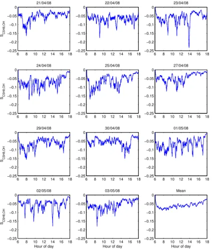
Figure 5 shows the intensity of segregation calculated by the model for each day of
20
available data for the OP3 campaign. SC5H8,OHis much less negative than suggested
in the studies of Butler et al. (2008) and Pugh et al. (2010) with a 10:00–18:00 LT mean
ofSC5H8,OH=−0.054 forts=10 min, resulting inkeffbeing 5.4% smaller thankC5H8,OH.
Figure 6 shows that the distribution ofSC5H8,OHduring OP3-1 is strongly skewed with
a tail towards the more negative values, with the median slightly less negative than
25
the mean atSC5H8,OH=−0.049. The 5th and 95th percentiles are SC5H8,OH=−0.104
andSC5H8,OH=−0.018 respectively. A large variation inSC5H8,OH is modelled over the
ACPD
10, 18197–18234, 2010Influence of variations in isoprene
concentration
T. A. M. Pugh et al.
Title Page
Abstract Introduction
Conclusions References
Tables Figures
◭ ◮
◭ ◮
Back Close
Full Screen / Esc
Printer-friendly Version Interactive Discussion
Discussion
P
a
per
|
Dis
cussion
P
a
per
|
Discussion
P
a
per
|
Discussio
n
P
a
per
|
Figure 7 shows thatSC5H8,OH is not strongly correlated with either the standard
de-viation (σ) or the mean (µ) of the isoprene concentration. However the combination of
these two statistics,σC5H8/µC5H8, i.e. the relative standard deviation, correlates strongly
with the intensity of segregation. This is likely due to the rate of increase of the overall
reaction rate of isoprene and OH,d RC5H8,OH/hC5H8i, decreasing with increasing
iso-5
prene concentration. Therefore a givenσC5H8will produce a greater range ofRC5H8,OH
overts, whenµC5H8is low. This indicator becomes less accurate asSC5H8,OHbecomes
more negative; we can find no simple explanation for this increase in scatter. It could be due to a combination of the skewness and kurtosis of the isoprene distribution, combined with the OH production rate and the size of the non-isoprene OH sink. One
10
feature of the plots in Fig. 7 is that, rather than a quasi-random scatter of data, the data points tend to arrange themselves in trajectories. This is most obvious with some of the outliers. This behaviour is a result of using running means over the input data, meaning that each point is influenced to some extent by the last, and should not be interpreted mechanistically.
15
The calculation ofSC5H8,OHpresented in this section is specific to the OP3
measure-ment site, as the relative deviation of the isoprene concentration will depend strongly upon the strength of the isoprene emission flux and upon the behaviour of the factors that make this flux heterogeneous in time and space, e.g. species distribution, canopy
venting, small-scale turbulence. This could lead to a large variation inSC5H8,OHat diff
er-20
ent sites. However two factors are worth noting here. The first is that the measurements
of Dlugi et al. (2010) for a forest in Germany and the modelled values ofSC5H8,OH
pre-sented here are very similar in magnitude despite their differing locations. The second
is that OP3 observed relatively small isoprene emissions compared to studies over the Amazon rainforest (Langford et al., 2010). At higher isoprene emissions the relative
25
deviation will be smaller for a similar amplitude of variation; from Fig. 7 this implies a
ACPD
10, 18197–18234, 2010Influence of variations in isoprene
concentration
T. A. M. Pugh et al.
Title Page
Abstract Introduction
Conclusions References
Tables Figures
◭ ◮
◭ ◮
Back Close
Full Screen / Esc
Printer-friendly Version Interactive Discussion
Discussion
P
a
per
|
Dis
cussion
P
a
per
|
Discussion
P
a
per
|
Discussio
n
P
a
per
|
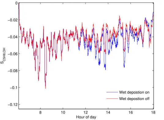
4.3 Sensitivity
Figure 7 demonstrates that the most important variables forSC5H8,OH identified by this
study are the magnitude and standard deviation of the isoprene concentration. To test how much the underlying photochemical characteristics of the atmosphere contribute
toSC5H8,OH the model was run using a normally-distributed, pseudo-randomly
gener-5
ated sequence of isoprene mixing ratios with a mean of 2 ppbv and a range of 0–4 ppbv, for a day of meteorological parameters. The result, shown by the blue line in Fig. 8,
reveals a relative minimum in the absolute magnitude ofSC5H8,OHat∼11:00 LT,
coinci-dent with the onset of precipitation, and hence a reduction in the non-isoprene OH sink due to the removal of highly soluble species such as peroxides. This clearly
demon-10
strates that the magnitude of the non-isoprene OH sink can have an impact on the
magnitude ofSC5H8,OH. In effect the additional sink dampens the size of OH′ caused
by a given C5H8′. In these simulations the effect onSC5H8,OHis small relative to those
induced by changes in the isoprene distribution (Fig. 5), as isoprene and its oxidation products dominated the OH sink during OP3. However, in a more polluted
environ-15
ment, correctly accounting for other OH sinks would become very important, although
of course, in such an environment, the importance ofSC5H8,OHwould be proportionally
smaller.
Plotting [OH] againstSC5H8,OH for the OP3 scenario suggests a correlation between
the two variables (not shown). However, this is not real; when the random isoprene time
20
series is used, no correlation is seen with [OH]. Therefore the apparent correlation in the OP3 scenario must be a result of the shape of the diurnal [OH] signal being similar to that of isoprene, since both are ultimately controlled by solar radiation. Furthermore, running the model using a constant photolysis rate, and hence constant photolytic
OH production, leads to deviation in SC5H8,OH only at the extreme ends of the day
25
compared to a run with normal photolysis. Hence [OH] cannot be determined to have
any significant predictive power forSC5H8,OH.
ACPD
10, 18197–18234, 2010Influence of variations in isoprene
concentration
T. A. M. Pugh et al.
Title Page
Abstract Introduction
Conclusions References
Tables Figures
◭ ◮
◭ ◮
Back Close
Full Screen / Esc
Printer-friendly Version Interactive Discussion
Discussion
P
a
per
|
Dis
cussion
P
a
per
|
Discussion
P
a
per
|
Discussio
n
P
a
per
|
might include a hitherto unconsidered OH formation mechanism, especially under
con-ditions of low NOxconcentrations (Lelieveld et al., 2008; Peeters et al., 2009). For the
purposes of this work, the most important factor in such an OH production mecha-nism is the time between initial isoprene oxidation and OH formation. If the extra OH
was formed very rapidly then it could decrease SC5H8,OH, as the OH loss caused by
5
isoprene oxidation would immediately be balanced to some extent by an OH source.
Running the model with the reaction of C5H8+OH modified to directly produce one
molecule of OH for each molecule of isoprene oxidised, as in Pugh et al. (2010),
re-sults inSC5H8,OH=0. However there is no known chemical scheme that could describe
such a production mechanism.
10
If additional OH is produced further down the isoprene oxidation chain, then the ad-ditional OH source is unlikely to be co-located with isoprene, instead being spread much more homogeneously across the boundary layer. To date, only Peeters et al. (2009) have proposed a detailed mechanism for how extra OH of the quantity appar-ently required by models might be formed. They point out a number of places in the
15
oxidation scheme where possible extra OH yields may occur. By far the most important route is by the photolysis of hydroperoxy-aldehyde compounds formed as a secondary oxidation product of isoprene. Peeters et al. (2009) estimate the photolysis frequency
for these compounds to be J=3×10⁻⁴s−1, with a quantum yield of 100%, giving a
lifetime of approximately 1 h. This suggests that OH formation via this route will not be
20
preferentially co-located with isoprene, as air parcels are highly unlikely to remain undi-luted over this time period. In this case, as it has already been demonstrated that the
OH concentration cannot be shown to have any direct effect onSC5H8,OH, OH recycling
on the timescale of an hour in the isoprene oxidation scheme is not expected to make
any difference to SC5H8,OH. To test this, the model was run for data from 30 April 2008
25
with an additional OH source one step further down the isoprene oxidation chain. The
result yields virtually no change inSC5H8,OH(not shown).
heteroge-ACPD
10, 18197–18234, 2010Influence of variations in isoprene
concentration
T. A. M. Pugh et al.
Title Page
Abstract Introduction
Conclusions References
Tables Figures
◭ ◮
◭ ◮
Back Close
Full Screen / Esc
Printer-friendly Version Interactive Discussion
Discussion
P
a
per
|
Dis
cussion
P
a
per
|
Discussion
P
a
per
|
Discussio
n
P
a
per
|
neous emission of NO, in addition to that of isoprene, led to a decreased magnitude
ofSVOC,OH, as an OH gradient formed as a result of the NO fluctuations counteracting
the effect of the VOC and OH segregation. NO is likely to be heterogeneously
dis-tributed as its principal source at the OP3 measurement site is biogenic below-canopy emissions. Therefore a spatial and temporal variation in both its original source, and
5
its release from the canopy is likely. No high temporal resolution measurement of NO
concentration were made during OP3, but 1 Hz measurements of NO2 concentration
made at 75 m on the measurement tower, show variations in NO2 concentration with
an amplitude of the same magnitude as the mean concentration, on a timescale of less
than 1 minute. As NO and NO2 are quickly inter-converted in the daytime boundary
10
layer, this suggests a heterogeneous distribution of NO within the boundary layer.
To test the effect of heterogeneous NO concentrations, three further runs were
car-ried out constrained to a randomly-generated normally distributed isoprene time-series. The first of these runs, N1, was constrained to a NO mixing ratio of 50 (10) pptv if isoprene mixing ratios were greater (less) than 2.5 (1.5) ppbv, and 30 pptv if isoprene
15
mixing ratios were between 1.5 and 2.5 ppbv. This produced an effect where high NO
concentrations were more typically co-located with high isoprene concentrations; an
effect that may well occur if coupling of the canopy to the BL is the primary reason for
heterogeneous concentration distributions. The second of these runs, N2, was iden-tical except a NO mixing ratio of 10 (50) pptv was used if isoprene mixing ratios were
20
greater (less) than 2.5 (1.5) ppbv, resulting in a scenario where high NO concentra-tions were typically anti-correlated with high isoprene concentraconcentra-tions. Finally N3 was constrained to a randomly-generated NO time-series that was entirely independent of isoprene.
Figure 9 shows the results for runs N1, N2 and N3, compared to the standard run
25
for that day. Run N1 shows a substantial decrease in segregation, with much less
negativeSC5H8,OH, as found by Krol et al. (2000). Indeed, at the ends of the day, when
OH production via photolysis is relatively small compared to production via the reaction
ACPD
10, 18197–18234, 2010Influence of variations in isoprene
concentration
T. A. M. Pugh et al.
Title Page
Abstract Introduction
Conclusions References
Tables Figures
◭ ◮
◭ ◮
Back Close
Full Screen / Esc
Printer-friendly Version Interactive Discussion
Discussion
P
a
per
|
Dis
cussion
P
a
per
|
Discussion
P
a
per
|
Discussio
n
P
a
per
|
caused by increased [NO] dominates over the effect caused by decreased isoprene.
Run N2 has the opposite effect, showing that NO concentrations anti-located with
isoprene concentrations could yield significantly more negative values ofSC5H8,OH. This
latter scenario appears unlikely in reality as, unless canopy-coupling proves to be the primary driver of heterogeneities in the BL leading to an N1-type scenario, it is likely
5
that the distributions of NO and isoprene in the BL will simply be different, showing
no kind of correlation. Run N3 demonstrates that if any heterogeneities in the NO concentration are independent of those in the isoprene concentration, then the typical
value ofSC5H8,OH should not be affected.
5 Conclusions
10
An approach has been described to model the intensity of segregation of isoprene and OH using high temporal resolution isoprene concentration data. The approach shows good agreement when compared with the only observations of isoprene and OH seg-regation available in the literature. When the method is applied to measurements made over the south-east Asian tropical rainforest during the OP3 campaign, an intensity of
15
segregation typically less negative than−0.15 is calculated. This is much less negative
than the−0.5 required by global and box models of atmospheric chemistry to reconcile
their OH and isoprene concentrations with measurements.
The model-calculated intensity of segregation for the OP3 rainforest scenario de-scribed in this paper appears robust, both to inhomogeneous concentrations of NO
20
and to potential OH recycling, unless NO anomalies are strongly correlated with those of isoprene or OH recycling happens virtually instantaneously following initial isoprene oxidation. Given that rapid isoprene concentration measurements have been made during several other field campaigns, it is suggested that the approach described here might be applied to estimate the intensity of segregation in those regions.
25
ACPD
10, 18197–18234, 2010Influence of variations in isoprene
concentration
T. A. M. Pugh et al.
Title Page
Abstract Introduction
Conclusions References
Tables Figures
◭ ◮
◭ ◮
Back Close
Full Screen / Esc
Printer-friendly Version Interactive Discussion
Discussion
P
a
per
|
Dis
cussion
P
a
per
|
Discussion
P
a
per
|
Discussio
n
P
a
per
|
concentrations at the expense of the fit to measured isoprene concentrations/fluxes. In order to attain an acceptable fit to both OH and isoprene concentrations a reduction in
kC5H8,OH was required. However this work shows that, at least for the rainforest
con-ditions observed during the OP3 campaigns in Malaysia, segregation of isoprene and OH can only be responsible for a minor fraction of the rate constant reduction required
5
to resolve the measurement-model discrepancy; hence either another justification for
thiskC5H8,OHreduction must be made or an alternative solution found.
In the light of the results presented here, it is suggested that the highest temporal resolution measurements for isoprene available are utilised in constrained modelling studies of atmospheric chemistry in areas where isoprene dominates the OH sink. If
10
high temporal resolution measurements of other species are co-located with the
iso-prene measurement (i.e. sufficiently close that they are very likely measuring within the
same air parcel) then it may prove advantageous to use these also.
Appendix A
The timescale for the OH concentration to reach a new steady state following a
pertur-15
bation in the isoprene mixing ratio from 2 ppbv to 3 ppbv (assuming no other OH sinks), is found by integrating the volume average conservation equation:
∂hOHi
∂t =POH−kC5H8,OHhOHihC5H8i (A1)
where,
POH=kO1D,H2OhO1DihH2Oi+kNO,HO2hNOihHO2i (A2)
20
to yield
t= "
−1
kC5H8,OHhC5H8i
ln|POH−kC5H8,OHhOHihC5H8i|
#hOHit
hOHi0
ACPD
10, 18197–18234, 2010Influence of variations in isoprene
concentration
T. A. M. Pugh et al.
Title Page
Abstract Introduction
Conclusions References
Tables Figures
◭ ◮
◭ ◮
Back Close
Full Screen / Esc
Printer-friendly Version Interactive Discussion
Discussion
P
a
per
|
Dis
cussion
P
a
per
|
Discussion
P
a
per
|
Discussio
n
P
a
per
|
wherehOHi0is the OH concentration att=0 andhOHitis the OH concentration at time
t, when the system is in steady state. At steady state∂hOHi/∂t=0, therefore,
POH=kC5H8,OHhOHihC5H8i (A4)
Hence thehOHit limit of Eq. (A3) is zero. When a POH=3.0×10
6
molecules cm−3s−1
is used,t=3 s. This value of POH is based upon midday typical midday values of the
5
components of Eq. (A2) during the OP3 campaign Hewitt et al. (2010). As the approach to steady state is exponential in nature, the majority of this change in [OH] due to
a perturbation in [C5H8] will occur within 1 second. This is demonstrated in Fig. A1
which shows an extract of the model time-series for C5H8(blue) and OH (green). Each
mark represents a model timestep of one second. It is clear that the OH response to a
10
change in C5H8 concentration occurs nearly entirely within the first timestep following
the change.
Acknowledgements. The authors wish to thank A. Jarvis for stimulating the discussion that led to this work and for helpful comments, P. Di Carlo for sharing his NO2data, and K. Ashworth for assistance with the analysis. We thank the Malaysian and Sabah Governments for their
per-15
mission to conduct research in Malaysia; the Malaysian Meteorological Department for access to the Bukit Atur Global Atmosphere Watch station; Waidi Sinun of Yayasan Sabah and his staff, Glen Reynolds of the Royal Society’s South East Asian Rainforest Research Programme and his staff, and Nick Chappell and Brian Davison of Lancaster University for logistical support at the Danum Valley Field Centre. The work was funded by the Natural Environment Research
20
Council Grants NE/D002117/1 and NE/E011179/1. This is paper number 508 of the Royal Society’s South East Asian Rainforest Research Programme.
References
Brown, P., Byrne, G., and Hindmarsh, A.: VODE – A Variable-coefficient ODE solver, Siam Journal on Scientific and Statistical Computing, 10, 1038–1051, 1989. 18209
25
ACPD
10, 18197–18234, 2010Influence of variations in isoprene
concentration
T. A. M. Pugh et al.
Title Page
Abstract Introduction
Conclusions References
Tables Figures
◭ ◮
◭ ◮
Back Close
Full Screen / Esc
Printer-friendly Version Interactive Discussion
Discussion
P
a
per
|
Dis
cussion
P
a
per
|
Discussion
P
a
per
|
Discussio
n
P
a
per
|
with the ECHAM5/MESSy chemistry-climate model: lessons from the GABRIEL airborne field campaign, Atmos. Chem. Phys., 8, 4529–4546, doi:10.5194/acp-8-4529-2008, 2008. 18199, 18200, 18201, 18202, 18211, 18216
Carslaw, N., Creasey, D., Harrison, D., Heard, D., Hunter, M., Jacobs, P., Jenkin, M., Lee, J., Lewis, A., Pilling, M., Saunders, S., and Seakins, P.: OH and HO2 radical chemistry in a
5
forested region of north-western Greece, Atmos. Environ., 35, 4725–4737, 2001. 18199, 18208
Dlugi, R., Berger, M., Zelger, M., Hofzumahaus, A., Siese, M., Holland, F., Wisthaler, A., Grab-mer, W., Hansel, A., Koppmann, R., Kramm, G., Mllmann-Coers, M., and Knaps, A.: Tur-bulent exchange and segregation of HOx radicals and volatile organic compounds above
10
a deciduous forest, Atmos. Chem. Phys., 10, 6215–6235, doi:10.5194/acp-10-6215-2010, 2010. 18202, 18209, 18210, 18211, 18212, 18228
Donovan, R., Hope, E., Owen, S., Mackenzie, A., and Hewitt, C.: Development and Application of an Urban Tree Air Quality Score for Photochemical Pollution Episodes Using the Birming-ham, United Kingdom, Area as a Case Study, Environ. Sci. Technol., 39, 6730–6738, 2005.
15
18208
Emmerson, K. M., MacKenzie, A. R., Owen, S. M., Evans, M. J., and Shallcross, D. E.: A Lagrangian model with simple primary and secondary aerosol scheme 1: comparison with UK PM10 data, Atmos. Chem. Phys., 4, 2161–2170, doi:10.5194/acp-4-2161-2004, 2004. 18208
20
Emmerson, K., Carslaw, N., Carpenter, L., Heard, D., Lee, J., and Pilling, M.: Urban at-mospheric chemistry during the PUMA campaign 1: Comparison of modelled OH and HO2 concentrations with measurements, J. Atmos. Chem., 52, 143–164, doi:10.1007/ s10874-005-1322-3, 2005. 18208
Emmerson, K. M., Carslaw, N., Carslaw, D. C., Lee, J. D., McFiggans, G., Bloss, W. J.,
Grave-25
stock, T., Heard, D. E., Hopkins, J., Ingham, T., Pilling, M. J., Smith, S. C., Jacob, M., and Monks, P. S.: Free radical modelling studies during the UK TORCH Campaign in Summer 2003, Atmos. Chem. Phys., 7, 167–181, doi:10.5194/acp-7-167-2007, 2007. 18208
Evans, M., Shallcross, D., Law, K., Wild, J., Simmonds, P., Spain, T., Berrisford, P., Methven, J., Lewis, A., McQuaid, J., Pilling, M., Bandy, B., Penkett, S., and Pyle, J.: Evaluation of
30
a Lagrangian box model using field measurements from EASE (Eastern Atlantic Summer Experiment) 1996, Atmos. Environ., 34, 3843–3863, 2000. 18208
ACPD
10, 18197–18234, 2010Influence of variations in isoprene
concentration
T. A. M. Pugh et al.
Title Page
Abstract Introduction
Conclusions References
Tables Figures
◭ ◮
◭ ◮
Back Close
Full Screen / Esc
Printer-friendly Version Interactive Discussion
Discussion
P
a
per
|
Dis
cussion
P
a
per
|
Discussion
P
a
per
|
Discussio
n
P
a
per
|
hydrocarbons on the tropospheric budget of carbon monoxide, Atmos. Environ., 34, 5255– 5270, 6th Scientific Conference of the International Global Atmospheric Chemistry Project (IGAC), Bologna, Italy, 13–17 September, 1999, 2000. 18199
Guenther, A., Hewitt, C., Erickson, D., Fall, R., Geron, C., Graedel, T., Harley, P., Klinger, L., Lerdau, M., McKay, W., Pierce, T., Scholes, B., Steinbrecher, R., Tallamraju, R., Taylor,
5
J., and Zimmerman, P.: A global model of natural volatile organic compound emissions, J. Geophys. Res., 100, 8873–8892, 1995. 18199
Hayward, S., Hewitt, C., Sartin, J., and Owen, S.: Performance characteristics and applications of a proton transfer reaction-mass spectrometer for measuring volatile organic compounds in ambient air, Environ. Sci. Tech., 36, 1554–1560, doi:10.1021/es0102181, 2002. 18203,
10
18204
Helfter, C., Phillips, G., Coyle, M., Di Marco, C., Langford, B., Whitehead, J., Dorsey, J., Gal-lagher, M., Sei, E., Fowler, D., and Nemitz, E.: Momentum and heat exchange above South East Asian rainforest in complex terrain, Atmos. Chem. Phys. Discuss., in preparation, 2010. 18202, 18206
15
Hewitt, C. N., Lee, J. D., MacKenzie, A. R., Barkley, M. P., Carslaw, N., Carver, G. D., Chappell, N. A., Coe, H., Collier, C., Commane, R., Davies, F., Davison, B., DiCarlo, P., Di Marco, C. F., Dorsey, J. R., Edwards, P. M., Evans, M. J., Fowler, D., Furneaux, K. L., Gallagher, M., Guenther, A., Heard, D. E., Helfter, C., Hopkins, J., Ingham, T., Irwin, M., Jones, C., Karuna-haran, A., Langford, B., Lewis, A. C., Lim, S. F., MacDonald, S. M., Mahajan, A. S., Malpass,
20
S., McFiggans, G., Mills, G., Misztal, P., Moller, S., Monks, P. S., Nemitz, E., Nicolas-Perea, V., Oetjen, H., Oram, D. E., Palmer, P. I., Phillips, G. J., Pike, R., Plane, J. M. C., Pugh, T., Pyle, J. A., Reeves, C. E., Robinson, N. H., Stewart, D., Stone, D., Whalley, L. K., and Yang, X.: Corrigendum to “Overview: oxidant and particle photochemical processes above a south-east Asian tropical rainforest (the OP3 project): introduction, rationale, location
char-25
acteristics and tools” published in Atmos. Chem. Phys., 10, 169–199, 2010, Atmos. Chem. Phys., 10, 563–563, doi:10.5194/acp-10-563-2010, 2010. 18202, 18218
Hewitt, C. N., MacKenzie, A. R., Di Carlo, P., Di Marco, C. F., Dorsey, J. R., Evans, M., Fowler, D., Gallagher, M. W., Hopkins, J. R., Jones, C. E., Langford, B., Lee, J. D., Lewis, A. C., Lim, S. F., McQuaid, J., Misztal, P., Moller, S. J., Monks, P. S., Nemitz, E., Oram, D. E.,
30
ACPD
10, 18197–18234, 2010Influence of variations in isoprene
concentration
T. A. M. Pugh et al.
Title Page
Abstract Introduction
Conclusions References
Tables Figures
◭ ◮
◭ ◮
Back Close
Full Screen / Esc
Printer-friendly Version Interactive Discussion
Discussion
P
a
per
|
Dis
cussion
P
a
per
|
Discussion
P
a
per
|
Discussio
n
P
a
per
|
18447–18451, doi:10.1073/pnas.0907541106, 2009. 18206, 18208
Hofzumahaus, A., Rohrer, F., Lu, K., Bohn, B., Brauers, T., Chang, C.-C., Fuchs, H., Holland, F., Kita, K., Kondo, Y., Li, X., Lou, S., Shao, M., Zeng, L., Wahner, A., and Zhang, Y.: Amplified Trace Gas Removal in the Troposphere, Science, 324, 1702–1704, doi:10.1126/science. 1164566, 2009. 18199, 18208
5
IUPAC: Evaluated kinetic data, http://www.iupac-kinetic.ch.cam.ac.uk/, last access: 19 March 2009. 18201
J ¨ockel, P., Tost, H., Pozzer, A., Br ¨uhl, C., Buchholz, J., Ganzeveld, L., Hoor, P., Kerk-weg, A., Lawrence, M. G., Sander, R., Steil, B., Stiller, G., Tanarhte, M., Taraborrelli, D., van Aardenne, J., and Lelieveld, J.: The atmospheric chemistry general circulation model
10
ECHAM5/MESSy1: consistent simulation of ozone from the surface to the mesosphere, At-mos. Chem. Phys., 6, 5067–5104, doi:10.5194/acp-6-5067-2006, 2006. 18199
Kanaya, Y., Cao, R., Kato, S., Miyakawa, Y., Kajii, Y., Tanimoto, H., Yokouchi, Y., Mochida, M., Kawamura, K., and Akimoto, H.: Chemistry of OH and HO2 radicals observed at Rishiri Island, Japan, in September 2003: Missing daytime sink of HO2and positive nighttime
cor-15
relations with monoterpenes, J. Geophys. Res., 112, D11308, doi:10.1029/2006JD007987, 2007. 18208
Kanaya, Y., Pochanart, P., Liu, Y., Li, J., Tanimoto, H., Kato, S., Suthawaree, J., Inomata, S., Taketani, F., Okuzawa, K., Kawamura, K., Akimoto, H., and Wang, Z. F.: Rates and regimes of photochemical ozone production over Central East China in June 2006: a box model
20
analysis using comprehensive measurements of ozone precursors, Atmos. Chem. Phys., 9, 7711–7723, doi:10.5194/acp-9-7711-2009, 2009. 18208
Kleffmann, J., Gavriloaiei, T., Hofzumahaus, A., Holland, F., Koppmann, R., Rupp, L., Schlosser, E., Siese, M., and Wahner, A.: Daytime formation of nitrous acid: A major source of OH radicals in a forest, Geophys. Res. Lett., 32, L05818, doi:10.1029/2005GL022524,
25
2005. 18210, 18211
Krol, M., Molemaker, M., and Vil `a Guerau de Arellano, J.: Effects of turbulence and hetero-geneous emissions on photochemically active species in the convective boundary layer, J. Geophys. Res., 105, 6871–6884, 2000. 18200, 18214, 18215
Kubistin, D., Harder, H., Martinez, M., Rudolf, M., Sander, R., Bozem, H., Eerdekens, G.,
Fis-30


![Fig. A1. Response of modelled [OH] to a change in the supplied C 5 H 8 . Each model time-point is marked by a dot.](https://thumb-eu.123doks.com/thumbv2/123dok_br/16465283.198612/38.918.101.610.112.497/fig-response-modelled-change-supplied-model-point-marked.webp)
