Concentrations and fluxes of biogenic volatile organic compounds above a Mediterranean macchia ecosystem in Western Italy

(1)

BGD

6, 2183–2216, 2009

BVOC concentrations and fluxes from Italy

B. Davison et al.

Title Page

Abstract Introduction

Conclusions References

Tables Figures

◭ ◮

Back Close

Full Screen / Esc

Printer-friendly Version

Interactive Discussion

Biogeosciences Discuss., 6, 2183–2216, 2009 www.biogeosciences-discuss.net/6/2183/2009/ © Author(s) 2009. This work is distributed under the Creative Commons Attribution 3.0 License.

Biogeosciences Discussions

Biogeosciences Discussionsis the access reviewed discussion forum ofBiogeosciences

Concentrations and fluxes of biogenic

volatile organic compounds above a

Mediterranean macchia ecosystem in

Western Italy

B. Davison1, R. Taipale2, B. Langford1, P. Misztal3,4, S. Fares5,*, G. Matteucci5, F. Loreto5, J. N. Cape3, J. Rinne2, and C. N. Hewitt1

1

Lancaster Environment Centre, Lancaster University, Lancaster LA1 4YQ, UK

2

University of Helsinki, Department of Physics, P.O. Box 68, 00014 Helsinki, Finland

3

Centre for Ecology & Hydrology, Bush Estate, Penicuik, Midlothian EH26 0QB, UK

4

School of Chemistry, University of Edinburgh, Edinburgh EH9 3JJ, UK

5

National Research Council, Institute of Agro-environmental and Forest Biology, Via Salaria km. 29 300, 00016 Monterotondo Scalo (Rome), Italy

*

now at: University of California, Department of Environmental Science, Policy, and Management, 137 Mulford Hall, Berkeley, CA 94720, USA

Received: 21 November 2008 – Accepted: 17 December 2008 – Published: 23 February 2009

Correspondence to: B. Davison (b.davison@lancaster.ac.uk)

(2)

BGD

6, 2183–2216, 2009

B. Davison et al.

Title Page

Tables Figures

◭ ◮

Back Close

Full Screen / Esc

Interactive Discussion Abstract

Emission rates and concentrations of biogenic volatile organic compounds (BVOCs) were measured at a Mediterranean coastal site at Castelporziano, approximately 25 km south-west of Rome, between 7 May and 3 June 2007, as part of the ACCENT-VOCBAS field campaign on biosphere-atmosphere interactions. Concentrations and

5

emission rates were measured using the disjunct eddy covariance method utilizing three different proton transfer reaction mass spectrometers (PTR-MS) for BVOC mix-ing ratio measurements and sonic anemometers for three-dimensional high-frequency wind measurements. Depending on the measurement period and the instrument, the median volume mixing ratios were 1.6–3.5 ppbv for methanol, 0.4–1.5 ppbv for

10

acetaldehyde, 1.0–2.5 ppbv for acetone, 0.10–0.17 ppbv for isoprene, and 0.18– 0.30 ppbv for monoterpenes. A diurnal cycle in mixing ratios was apparent with day-time maxima for methanol, acetaldehyde, acetone, and isoprene. The median fluxes were 370–440µg m−2

h−1

for methanol, 180–360µg m−2

h−1

for acetaldehyde, 180– 450µg m−2h−1for acetone, 71–290µg m−2h−1 for isoprene, and 240–860µg m−2h−1

15

for monoterpenes.

1 Introduction

Emissions of biogenic volatile organic compounds (BVOCs) play an important role in atmospheric chemistry. Oxidation of VOCs (both biogenic and anthropogenic) in a NO_x-rich atmosphere may lead to the production of tropospheric ozone, which has

20

impacts on human health and can cause damage to crops, forest ecosystems, and buildings (e.g. Sillman et al., 1999; Fowler et al., 2008).

In Mediterranean areas, where both emission and oxidation rates of BVOCs are high, production of ozone and particles from BVOC precursors represent a significant air quality challenge. Previous measurements have shown that isoprene and

monoter-25

(3)

BGD

6, 2183–2216, 2009

B. Davison et al.

Title Page

Tables Figures

◭ ◮

Back Close

Full Screen / Esc

(Helmig et al., 1999). However, little is known about emissions of oxygenated com-pounds, such as methanol and acetone, from these ecosystems. BVOC emissions are strongly regulated by variations in light and temperature (e.g. Guenther et al., 1993). Nonetheless, the light and temperature dependent emission algorithms are still limited by uncertainties, particularly of the basal emission rates on which they depend.

5

To better understand the processes controlling photochemical pollution episodes, re-gional and global scale BVOC emission models have been developed. Until recently, many model estimates for biogenic emissions from Mediterranean type ecosystems (Guenther et al., 1995; Simpson et al., 1999; Owen and Hewitt., 2000), which could in-clude regions of Chile, California, South Africa, Australia, and Europe, were calculated

10

using basal emission rates determined for Californian Mediterranean type ecosystems only (Owen et al., 1997). Isoprene and monoterpene emissions both tend to be very species specific, which generates considerable uncertainty in the model.

In recent years, e_fforts have been made to determine emission rates for a number of Mediterranean type ecosystems. In Europe, BVOC emissions in the Mediterranean

15

area were extensively studied as part of the Biogenic Emissions in the Mediterranean Area (BEMA) project (Bertin et al., 1997; Ciccioli et al., 1997; Kesselmeier et al., 1997; Owen et al., 1997, 2001, 2002; Seufert et al., 1997; Street et al., 1997; Valentini et al., 1997). The BEMA project focused on emissions from the Castelporziano nature reserve near Rome, Italy. As the site comprised a number of vegetation types, both

20

species specific and averaged ecosystem (forest, pseudosteppe, or macchia) emission rates could be calculated, which allowed improved modelled BVOC emission estimates within this region.

Since the BEMA campaigns there have been improvements in analytical techniques for VOCs. The advent of proton transfer reaction mass spectrometry (PTR-MS) has

25

(4)

BGD

6, 2183–2216, 2009

B. Davison et al.

Title Page

Tables Figures

◭ ◮

Back Close

Full Screen / Esc

the pptv (parts per trillion by volume) level with a response time of seconds or less has led to the use of the PTR-MS instrument in micrometeorological eddy covariance flux measurement methods such as conventional eddy covariance (e.g. Karl et al., 2001), disjunct eddy covariance (DEC; Rinne et al., 2001), and disjunct eddy covariance with continuous sampling flow (DEC_cf), sometimes also called virtual disjunct eddy

covari-5

ance (Karl et al., 2002). The DEC_cf method was utilized in this study. The PTR-MS measured mixing ratios of different VOCs sequentially, which leads to a disjunct data set. Once these data were synchronized with the high-frequency wind data, BVOC fluxes could be calculated for the footprint area.

This paper presents the results of the mixing ratio and flux measurements made

10

at Castelporziano within the frame of the ACCENT-VOCBAS campaign on biosphere-atmosphere interactions (for an overview, see Fares et al., 2009). Three different PTR-MS instruments were utilized in the measurements between 7 May and 3 June 2007. During the first measurement period (7–14 May), two measurement setups were oper-ated simultaneously by Lancaster University (LU) and the Centre for Ecology &

Hydrol-15

ogy Edinburgh (CEH), and during the latter period (20 May–3 June), the measurements were carried out in cooperation between the National Research Council of Italy (Con-siglio Nazionale delle Ricerche, CNR) and the University of Helsinki (UH).

2 Methods

2.1 Measurement site

20

The Presidential Estate of Castelporziano (41◦40′49′′N, 12◦23′31′′E) is located about 25 km to the south-west from the city centre of Rome, Italy. It covers an area of 60 km2 and has a coastline of 5 km (for a detailed description of the site see Fares et al., 2009). Due to restricted public access, a number of Mediterranean ecosystem types have been preserved (e.g. macchia and pseudosteppe). The estate has few roads

25

(5)

BGD

6, 2183–2216, 2009

B. Davison et al.

Title Page

Tables Figures

◭ ◮

Back Close

Full Screen / Esc

road. The smaller SS601 public road transects the southern edge creating a boundary between the high and low macchia. The low macchia was chosen as the site for this study.

A measurement tower was erected in a slight valley depression separated from the sea by two lines of sand dunes. The vegetation in the vicinity of the tower consisted

5

mainly ofArbutus unedo, Rosmarinus officinalis, Quercus ilex, Phillyrea angustifolia, and Erica multiflora (Fares et al., 2009). The average canopy height, 1.2 m, was estimated by calculating the weighted average of the average heights of these main species, which covered 80% of the total area of 1070 m2around the tower. The weight factor was the proportion of the total area covered by a particular species. A forest of

10

23 km2 dominated by Holm oak (Quercus ilex) was located approximately 1 km to the north-east.

2.2 Measurement setup and procedure

Commercial PTR-MS instruments (Ionicon Analytik GmbH) were used in the measure-ments. LU and CNR-UH used two instruments which both featured two turbomolecular

15

pumps, a heated silica steel inlet system, and a 9.6 cm long stainless steel drift tube. According to the manufacturer, the response time was about 1 s for these instruments. The PTR-MS used by CEH contained a third turbomolecular pump and its response time was about 0.2 s.

The measurement setup used by LU and CEH during the first measurement period

20

consisted of a three-dimensional ultrasonic anemometer (Gill Instruments Ltd., So-lent R2), and two PTR-MS instruments. LU also used a humidity sensor (Honeywell In-ternational, Inc., HIH-4000-001) and an ozone monitor (2B Technologies, Inc., 205 dual beam). The anemometer was mounted at 5 m above ground on the south-west corner of the measurement tower. This position gave a fetch of approximately 300 m to the

25

(6)

BGD

6, 2183–2216, 2009

B. Davison et al.

Title Page

Tables Figures

◭ ◮

Back Close

Full Screen / Esc

Teflon tube was used as the main sampling line taking air at 18 l min−1 from a position 30 cm below the anemometer.

The PTR-MS instruments sampled from the main sampling line at 0.25 l min−1

. They were optimised to an E/N ratio of 128 Td using a drift tube pressure, temperature, and voltage of 2.02 hPa, 45◦C, and 500 V, respectively. The reaction time was 100µs and

5

the count rate of H₃O+H₂O ions was 1.2–2.6% of the count rate of H₃O+ ions, which was (1.6–3.1)×106counts s−1. The data from the ultrasonic anemometer and PTR-MS

were logged into the same computer using a programme written in LabView (National Instruments Corp.). The humidity sensor (Honeywell, HIH4000-001) and ozone mon-itor sampled from the main line at a rate of 0.5 Hz and ancillary measurements of air

10

pressure, temperature, photosynthetically active radiation, and CO2 and H2O mixing

ratios were recorded by an environmental gas analyser (PP Systems, EGM-4) with a time resolution of 20 s.

Both PTR-MS instruments measured in three modes: flux, ambient mixing ratio, and zero air. Each instrument measured zero air for a five-minute period each hour

15

followed by a 25-min flux measurement period and then a 5-min mixing ratio measure-ment period before a second 25-min flux measuremeasure-ment period. Zero air was generated by passing ambient air through a glass tube containing a platinum catalyst powder at 0.5 l min−1. In the flux measurements, the PTR-MS measurement cycle contained eight masses and six of them were related to BVOCs (Table 1). The PTR-MS

integra-20

tion, or dwell, time was 0.2 s for each BVOC-related mass and the total measurement cycle length was 1.4 s. This corresponded to approximately 1070 measurements over the 25-min flux averaging period. In the ambient mixing ratio measurements, seven BVOC-related masses were measured within a PTR-MS measurements cycle of 7.1 s (Table 1) with an integration time of 1 s for each VOC-related mass.

25

(7)

BGD

6, 2183–2216, 2009

B. Davison et al.

Title Page

Tables Figures

◭ ◮

Back Close

Full Screen / Esc

ground and the PTR-MS was housed in the air-conditioned cabin. The main sampling line was 25 m long, its inner diameter was 8 mm, and it was made of Teflon (PTFE). A continuous flow of 25 l min−1 was used in the main line and a side flow of 0.12 l min−1 was taken into the PTR-MS via a 1.5 m long PTFE tube, which had an inner diameter of 1.6 mm. A PTFE filter (1µm pore size, LI-COR, Inc., part number 9967-008) was

5

installed in front of the PTR-MS inlet to prevent particles from entering the instrument. The operating parameters of the PTR-MS were held constant during the measure-ment period (20 May–3 June), except for the secondary electron multiplier voltage, which was optimized before every calibration. The drift tube pressure, temperature, and voltage were 2.2 hPa, 55◦C, and 600 V, respectively. The parameter E/N was about

10

130 Td and the reaction time was about 97µs. The count rate of H₃O+H₂O ions was 1–9% of the count rate of H3O+ions, which was (2.9–5.5)×10

6

counts s−1.

The wind measurements were conducted continuously at a sampling frequency of 20 Hz and the data were recorded on a different computer than the BVOC data. The BVOC measurement procedure was controlled with the Balzers Quadstar 422

soft-15

ware of the PTR-MS and it contained two hour-long sequences. Every second hour was allocated to the flux measurements. The PTR-MS measurement cycle consisted of 15 masses and 12 of them were related to BVOCs (Table 1). The measurement cycle length was 13.3 s and the cycle was repeated 264 times an hour. The PTR-MS integration time was 1 s for each BVOC-related mass. The other hour-long sequence

20

consisted of zero air measurements and ambient mixing ratio measurements. In the zero air measurements, VOC-free air produced from ambient air with a zero air gener-ator (catalytic converter, Parker Hannifin Corp., ChromGas Zero Air Genergener-ator 1001) was fed into the PTR-MS to determine BVOC background signals of the instrument. Zero air was measured for about 12.5 min (20 cycles) and then the PTR-MS was set to

25

(8)

BGD

6, 2183–2216, 2009

B. Davison et al.

Title Page

Tables Figures

◭ ◮

Back Close

Full Screen / Esc

measurements of ambient air. The scan range was 40–250 amu and the integration time was 2 s for each mass.

2.3 Calculation of BVOC volume mixing ratios

The PTR-MS instruments of LU and CEH were calibrated against the same gas stan-dard, which contained methanol, acetaldehyde and acetone at a mixing ratio of 1 ppmv.

5

The gas standard was prepared by diluting known volumes of the gas standard with zero hydrocarbon free air in Tedlar bags. These were then used to calibrate the PTR-MS over the range of 2–700 ppbv. In the first period, BVOC calibrations were done on 6 and 13 May.

LU and CEH calculated the normalized sensitivities for isoprene and monoterpenes

10

(Table 2) using the proton transfer reaction rate coefficients of Zhao and Zhang (2004) and the instrument specific transmission coe_fficients which were calculated following the procedure described by Wilkinson (2006).

The PTR-MS of CNR-UH was calibrated three times during the measurement period: on 20, 25, and 31 May. These calibrations were performed with gas standards prepared

15

by diluting pure liquid standards in nitrogen and analysed with a gas chromatograph-mass spectrometer at CNR. The monoterpene mixing ratio in the standard gas was 2.35 ppmv and the mixing ratios of methanol, acetaldehyde, acetone, and isoprene were 1 ppmv. The monoterpenes used in the calibrations were α-pinene (1 ppmv), limonene (1 ppmv), and ocimene (350 ppbv). The standard gas was diluted with zero

20

(9)

BGD

6, 2183–2216, 2009

B. Davison et al.

Title Page

Tables Figures

◭ ◮

Back Close

Full Screen / Esc

VOC volume mixing ratios (VMR) were calculated using a similar approach by all groups as described by Taipale et al. (2008):

VMR= I(RH

+₎

norm Snorm

, (1)

where Snorm is the normalized sensitivity in units of normalized counts s− 1

ppbv−1 (ncps ppbv−1_{). The normalized count rate of RH}+ _{ions is}

5

I(RH+)norm=I(RH+)

_I_(H

3O+)+I(H3O+H2O)

Inorm

−1_p

drift

p_norm −1

−1n n P

i=1

I(RH+)zero,i

_I_(H

3O+)zero,i+I(H3O+H2O)zero,i

Inorm

−1

_p

drift,zero,i

p_norm −1

,

(2)

where I(RH+), I(H3O+), and I(H3O+H2O) are the count rates of RH+, H3O+, and

H3O+H2O ions, pdrift is the drift tube pressure, and nis the number of zero air

mea-surement cycles. The sum of the primary and water cluster ion count rate is normalized to a count rate ofInorm=10

6

cps and the drift tube pressure is normalized to a pressure

10

ofpnorm=2 hPa. The primary ion count rate was determined using the signal of the

primary ion isotopes detected at 21 amu (M21). In the flux measurements, the wa-ter cluswa-ter ion count rate was derived from the wawa-ter cluswa-ter ion signal detected at M37, while in the ambient mixing ratio measurements it was derived from the signal of the water cluster ion isotopes detected at M39. The contribution of the oxygen

iso-15

(10)

BGD

6, 2183–2216, 2009

B. Davison et al.

Title Page

Tables Figures

◭ ◮

Back Close

Full Screen / Esc

2.4 Calculation of BVOC fluxes

VOC fluxes were measured with the DEC_cf. To determine the measured fluxes,F_m, a covariance function was calculated for each compound:

F_m(∆t)= 1

N

N X

i=1

w′ _i ₋_∆_t

∆t_w

c′₍_i₎_. ₍₃₎

In this equation, w′₌_w

−w¯ is the momentary deviation of the vertical wind speed, w,

5

from its average,c′

=c−c¯ is that of the BVOC mass concentration, ∆t is the lag time

between the wind and concentration measurements, ∆t_w is the sampling interval in the wind measurements, andNis the number of PTR-MS measurement cycles during the flux averaging time. LU and CEH used a flux averaging time of 25 min which cor-responded toN=1070. The averaging time of CNR-UH was 30 min, corresponding to

10

N=132. The sampling interval was 0.05 s in the wind measurements of both LU-CEH and CNR-UH.

To aid identification of the lag time, LU used the data from the humidity sensor con-nected to the main sampling line at the same point as both PTR-MS instruments. The humidity data were combined with the vertical wind speed data, allowing a correlation

15

function to be applied and the lag time to be estimated. A six-second time window was used to refine the lag time. A BVOC flux measurement was rejected if no clear peak was detected above the general noise of the covariance function within the time window.

The CEH group adopted a variable lag time approach, assuming there were several

20

sources of delays. A procedure for estimating the lag time by performing the cross-correlation between the vertical wind speed component and the BVOC signal on all individual half-hour periods for each compound separately was used. Visual assess-ments of both the position and the quality of the peak in the covariance function were made for all the compounds measured in the flux mode within a 10 s window. The

re-25

(11)

BGD

6, 2183–2216, 2009

B. Davison et al.

Title Page

Tables Figures

◭ ◮

Back Close

Full Screen / Esc

the lag times for a givenm/zshould not differ by more than a cycle length. Normally, variability of 2 s deviation from expected mean lag time was considered acceptable.

In the flux measurements by CNR-UH, the wind data were recorded on a different computer than the PTR-MS data. This means that there was an uncertainty in the timing of the wind and concentration time series in addition to the lag time due to

5

the residence time of the sample air in the sampling lines. Therefore, the covariance functions were calculated for a rather wide lag time interval of ±3 min, using a time

step of 0.05 s. To facilitate the identification of the lag time, the covariance function was calculated also for H3O+H2O ions detected at M37 (Rinne et al., 2007). Since the

signal of these water cluster ions is high and depends on the ambient water vapour

10

mixing ratio (Ammann et al., 2006), there usually is a clear maximum in a covariance function related to daytime measurements. If a clear maximum could be identified from the covariance function of M37, a lag time window of±13.3 s around the maximum

was chosen. Finally, the BVOC fluxes were determined by finding the maxima of the respective covariance functions within the lag time window. Normally, CNR-UH could

15

calculate the fluxes from the measurements conducted between 08:00 and 21:00 LT. Two micrometeorological quality criteria were employed in the post-processing of the flux data of LU, CEH, and CNR-UH. A flux measurement was discarded if it was obtained in stable conditions or if the friction velocity was below 0.2 m s−1_{. The}

high-frequency attenuation of the measured flux caused by the response time of the

PTR-20

MS was estimated from the equation.

Fm

F =

1

1+ 2πn_mτu¯

(z−d)α

, (4)

whereF is the non-attenuated flux,τis the response time, and ¯uis the average wind speed at the measurement height, z (Horst, 1997). For neutral and unstable strat-ification, the dimensionless frequency at the cospectral maximum is n_m=0.085 and

25

the exponent is α=7/8. The displacement height was calculated using the relation

(12)

BGD

6, 2183–2216, 2009

B. Davison et al.

Title Page

Tables Figures

◭ ◮

Back Close

Full Screen / Esc

response time was 1 s for the LU and CNR-UH instruments and 0.2 s for the CEH in-strument. The range of the high-frequency attenuation was 0.62–0.98 for the LU data, 0.87–0.99 for the CEH data, and 0.45–0.97 for CNR-UH data. The median values were 0.78, 0.93, and 0.71, respectively.

2.5 Identification of BVOCs

5

To assist identification of the compounds contributing to the masses measured by PTR-MS, occasional measurements with gas-chromatographic methods were performed during the first measurement period 7–13 May. The technique has been described in more detail by Davison et al. (2008). At a flow rate of 200 ml min−1 a total volume of 4 l air was sampled through stainless steel sampling tubes packed with Tenax and

10

Carbopack B to pre-concentrate VOCs. These samples were analysed by thermal desorption (Perkin Elmer Turbomatrix thermal desorption system) and GC-MS (Perkin Elmer Turbomass Gold GC-MS). The compounds were separated on an Ultra 2 column (50 m×0.2 mm, I.D., 0.11µm P/N 19091-005 Agilent Technologies). Compound

iden-tification was by standards whenever possible and Wiley and NIST spectral libraries.

15

Light compounds, usually below C4, are readily lost in the pre-concentration step on

the Tenax tubes and so are not reliably detected by this method. Measurements using Tenax tubes were also made during the second measurement period and are reported in the companion paper (Fares et al., 2009).

3 Results and discussion

20

3.1 Weather during the campaign

(13)

BGD

6, 2183–2216, 2009

B. Davison et al.

Title Page

Tables Figures

◭ ◮

Back Close

Full Screen / Esc

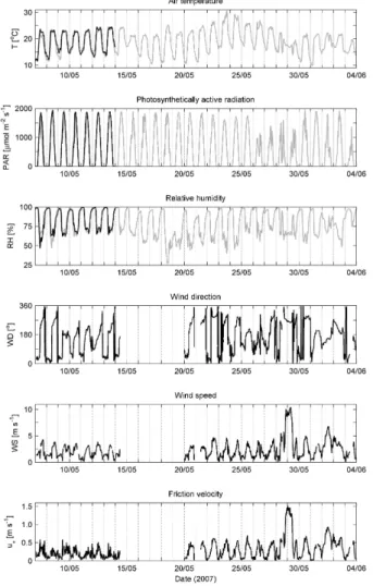
the two sites shows a good agreement vindicating the use of measurements from the CarboEurope data set. During the first part of the campaign (7–14 May), the site experienced a diurnal sea breeze with onshore winds from 180◦to 270◦during the day

from around 11:00 to 19:00 LT and an offshore or land breeze from a northerly direction dominating from 03:00 or 04:00 until 11:00 LT. The wind speed was between 0.1 and

5

4.3 m s−1, averaging 1.8 m s−1. The highest wind speed was observed around 13:00 LT with the lowest coinciding with the sea-land breeze reversal during the evening. Prior to the start of the campaign the region experienced heavy rain and flash flooding. From 1 to 7 May the site experienced 18.5 mm of rain of which 11.7 mm fell overnight on 4 May. This unsettled weather gradually gave way to clear skies and warmer conditions. The

10

ambient temperature ranged from 13 to 24◦_{C which gradually increased between 7 and}

14 May.

During the second part of the campaign 20 May–3 June, the wind direction varied typically from 180◦ _{to 280}◦ _{between 09:00 and 21:00 LT and from 50}◦ _{to 150}◦ _during

the night. The wind speed ranged from 0.1 to 10.4 m s−1. The highest values were

15

observed between 14:00 and 19:00 LT and the lowest between 21:00 and 02:00 LT. The air temperature ranged from 10 to 31◦_{C and the typical values were 19–23}◦_{C in}

the daytime and 15–19◦C at night. The daily maximum values of photosynthetically active radiation were around 1400–1900µmol m−2s−1. The cumulative rainfall during 20 May–3 June was 22 mm. The most intensive showers took place on 28 and 29 May

20

and there was a period of continuous rain on 3 June.

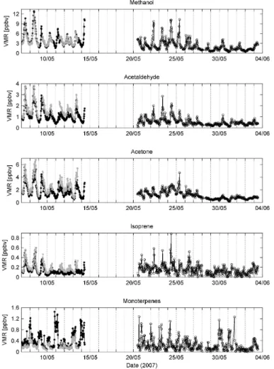
3.2 VOC mixing ratios

Figure 2 shows the half-hour averages of the mixing ratios of methanol, acetaldehyde, acetone, isoprene, and monoterpenes measured with the PTR-MS instruments of LU, CEH and CNR-UH. In general, the agreement between the LU and CEH instruments

25

(14)

BGD

6, 2183–2216, 2009

B. Davison et al.

Title Page

Tables Figures

◭ ◮

Back Close

Full Screen / Esc

were calculated using PTR-MS transmission factors as gas standards were not avail-able for these compounds.

The results from the two periods in early and late May exhibit similar overall trends though the average mixing ratios of methanol, acetaldehyde, and acetone were slightly lower during the second period.

5

Table 3 shows a summary of the concentration results from the two measurement periods. During the first measurement period (7–14 May 2007) concentrations of all species were highest during the first few days. Methanol emissions are known to be influenced by abiotic stress factors such as elevated ozone levels, drought, flood-ing and mechanical leaf woundflood-ing (Fukui and Doskey, 1998; Holzflood-inger et al., 2000;

10

Beauchamp et al., 2005; Karl et al., 2005; Brunner et al., 2007; Penuelas et al., 2005) as well as leaf age, with higher emissions typical of young developing leaves (Nemecek-Marshall et al., 1995). Whether the elevated concentration levels observed over the first few days of the campaign were due to the heavy rain encountered during this period or disturbance of the site during setting up is unclear but there are also

no-15

tably higher concentrations during the early part of the second period of the campaign (20 May to 3 June 2007), suggesting these elevated concentrations may be related to the inevitable vegetation disturbance during setting up.

Methanol was the most abundant compound measured, and along with acetalde-hyde, acetone and isoprene showed a similar trend with a clear diurnal cycle with a

20

daytime maximum. Monoterpenes showed a diurnal trend but with a night time maxi-mum. Measurements over crop fields have also shown methanol to be one of the most abundant biogenically emitted VOCs (Warneke et al., 2002; Fall, 2003; Schade and Custer, 2004; Davison et al., 2008). Measurements during the original BEMA cam-paigns observed oxygenated compounds emitted from pine and oak species. Acetic

25

(15)

BGD

6, 2183–2216, 2009

B. Davison et al.

Title Page

Tables Figures

◭ ◮

Back Close

Full Screen / Esc

campaign with ambient concentrations vary from 0 to 7 ppbv with a daytime maximum. This has proved to be in keeping with the measurements from this campaign where a 4 ppbv daytime maximum concentrations was observed measured using PTR-MS.

On a daily basis, concentrations of methanol, acetaldehyde, acetone and iso-prene typically began to increase at around 07:00 LT. Methanol and acetaldehyde both

5

peaked in the early morning (10:00 LT) with a secondary afternoon peak followed by a gradual decrease throughout the rest of the day. Similar trends were observed by Kesselmeier et al. (1997) for acetic and formic acid released from oak and related to transpiration patterns. The strong stomatal dependency of the emission of solu-ble compounds, such as methanol has been highlighted previously (Niinemets et al.,

10

2004).

Measurements of acetone, although similar to those of methanol and acetaldehyde, showed some differences, such as a sharp decline in concentration at around 19:00 LT. Isoprene concentrations increased throughout the afternoon after an initial peak at 08:00 LT, to reach a maximum at 14:00 LT, before decreasing sharply, similar to

ace-15

tone. Ozone measurements at the site showed a diurnal trend with a daytime maximum occurring a few hours after the maximum in BVOC concentrations. This maximum prob-ably relates more to the change in direction of the sea-land breeze than to any reaction with VOCs emitted from the vegetation.

The low molecular weight compounds (methanol, acetaldehyde, acetone and

iso-20

prene), as well as showing similar trends, had good correlation coefficients between each compound, ranging from anR2value of 0.52 between methanol and isoprene to anR2of 0.8 for acetone and acetaldehyde suggesting their similar origins.

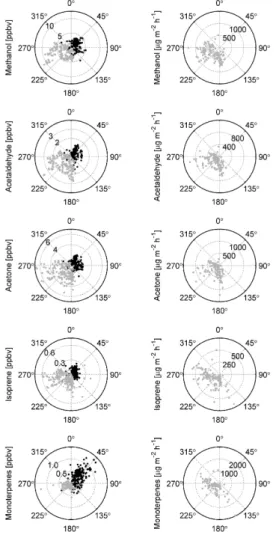
A wind rose of BVOC concentrations and fluxes (Fig. 3) shows a scatter of con-centrations around the site with predominance of daytime concon-centrations coming from

25

(16)

BGD

6, 2183–2216, 2009

B. Davison et al.

Title Page

Tables Figures

◭ ◮

Back Close

Full Screen / Esc

noticeable breeze effect than during the second measurement period. A natural for-est of Holm oak, a known monoterpene emitter, and a plantation of stone pine were located in this direction. This suggests that much of the monoterpenes measured during the campaign did not originate within the footprint of the flux area but were hor-izontally advected into the site. The highest monoterpene concentrations during both

5

campaign periods were observed at night once the wind had switched direction and the land breeze dominated, bringing air from the Holm oak forest to the measurement site. At night Holm oaks continue to emit monoterpenes although at much lower rates than during the day (Staudt and Bertin, 1998; Grote et al., 2006), but rapid removal of the compounds by reaction with light induced hydroxyl radicals ceases. Monoterpene

10

emission from pines is not light-dependent and is sustained or even stimulated at night (Owen et al., 1997; Staudt et al., 1997).

A similar directional trend is not apparent in the monoterpene flux (Fig. 3), confirming the source is outside the flux footprint area. This also agrees with the findings from Tenax tube samples collected during the first period of the campaign from plants within

15

the flux footprint area which showed only low levels of monoterpenes being emitted by the species occurring in the footprint area.

Monoterpene emissions were higher during the second period of the campaign, both as measured by PTR-MS over the sampling site and from leaf cuvette measurements of specific plant species. This may be related to the temperature, which was

approx-20

imately 3◦C higher during the second part of the campaign (Fares et al., 2009), and the more advanced phenological state of the plants in the flux footprint area. Isoprene emission is known to be dependent on leaf development (Wiberley et al., 2005), but similar evidence is missing for monoterpene emitters.

The concentrations measured simultaneously by the CEH and LU PTR-MS

instru-25

(17)

BGD

6, 2183–2216, 2009

B. Davison et al.

Title Page

Tables Figures

◭ ◮

Back Close

Full Screen / Esc

indicates that external standards are required for the highest accuracy of results, as the di_fferences between calculated and measured sensitivities have been reported to be up to a factor of 2 (Warneke et al., 2002; de Gouw and Warneke, 2007).

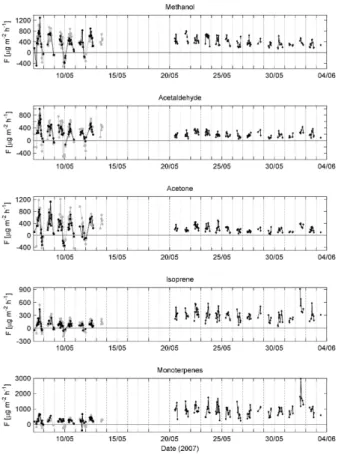
3.3 BVOC fluxes

Emissions of all five monitored compounds were observed from the macchia. Figure 4

5

shows the fluxes measured during the first and second period of the campaign. Emis-sion rates were highest during mid to late afternoon and lowest during the night. This reflects the diurnal cycle of the biological and physical processes affecting the emis-sions. Most of the night time flux data were rejected due to the quality criteria. This reflects the low wind speeds and weak mixing encountered at night. Monoterpene

10

fluxes also showed a daytime maximum, in contrast to the concentration measure-ments, which had higher night time values due to monoterpene-rich air being advected into the measurement area from the nearby Holm oak and pine areas when the land breeze became dominant at night.

The comparison of fluxes measured by CEH and LU showed similar overall trends

15

with some night time deposition observed. Note however, that night time flux measure-ments are often associated with large degrees of uncertainty due to the stable atmo-spheric conditions and low wind speeds that often occur at night. Night time fluxes have largely been filtered out from the flux measurements presented by CNR-UH for the second measurement period. Median day and night time mixing ratio and flux data

20

are presented in Table 3.

Methanol fluxes closely followed the diurnal profile of light and temperature with emissions peaking at around mid-day. The concentration measurements showed a slight difference peaking in early morning, before declining steadily throughout the afternoon. Plant physiology controls the emissions of methanol from

vege-25

(18)

BGD

6, 2183–2216, 2009

B. Davison et al.

Title Page

Tables Figures

◭ ◮

Back Close

Full Screen / Esc

(Mudgett and Clarke, 1993). The emission of methanol is controlled via the transpi-ration stream, which is itself governed by light and leaf temperature (which explains the close agreement with temperature), as well as stomatal conductance (Niinemets et al., 2004). Methanol formation resulting from catabolism can also occur during the night when the stomata are closed so leading to a methanol build up in the plant, which

5

is released in a burst when the stomata open in the morning. This venting process has been suggested by Cojocariu and Hewitt (C. Cojocariu and N. Hewitt, personal communications, 2008) but is not thought to be the reason for the morning maxima in VOC concentrations seen in this study, as similar peaks are not seen in the flux. Instead, it is assumed that the concentration increase is related to an accumulation of

10

early morning emissions into the shallow residual nocturnal boundary layer. Like the methanol concentration data, the flux data showed elevated values at the beginning of the campaign which are assumed to be related to plant damage during setup and to presence of a higher fraction of expanding leaves.

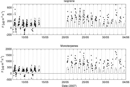
Isoprene and monoterpene emission estimates were calculated using the G97

algo-15

rithms from Guenther (1997) which assumes light and temperature dependent isoprene and monoterpene emitters. Summer time basal emission rates of 563µg m−2

h−1

for isoprene (Owen et al., 1998) and 1199µg m−2h−1for monoterpene (Fares et al., 2009) were used and a biomass density of 225 g m−2 for the measurement site from Fares et al. (2009). Light and temperature values from 7 May to 3 June were taken from the

20

CarboEurope data set.

As can be seen from Fig. 5 the comparison of modelled and measured isoprene fluxes using the DEC_cf technique showed reasonable agreement, with higher mod-elled flux values being calculated for the second part of the campaign in keeping with the measurements. During the first part of the campaign, the daytime medians of the

25

measured isoprene fluxes were 96.6 and 160µg m−2_h−1 _{from LU and CEH}

(19)

BGD

6, 2183–2216, 2009

B. Davison et al.

Title Page

Tables Figures

◭ ◮

Back Close

Full Screen / Esc

isoprene fluxes measured in the second part of the campaign are also observed in the model results. The daytime medians of the measured isoprene and monoterpene fluxes were 317 and 963µg m−2h−1, respectively. The daytime medians of the model results were 223 and 475µg m−2h−1.

The fluxes derived by the two groups in the first period agree reasonably well,

show-5

ing the scale of uncertainty caused by individual lag time determination, which was done separately by each group, leading to a slight difference in the amount of data rejected due to an unclear lag time. The negative fluxes may be the result of flux di-vergence, with considerable uncertainties from advection and general low turbulence conditions. The fluxes of monoterpenes were derived differently by both groups in the

10

first period. For example, in the processing of CEH data, the lag times form/z81 and

m/z137 were derived independently, while in the LU analysis the lag times were de-rived for the sum of the fragments. This led to coincidental good agreement in values, but in fact the LU flux should be higher, considering the higher concentrations that were reported.

15

In the comparison of the two periods one needs to take into account the more ad-vanced phenological stage of macchia vegetation, expecting higher VOC emissions.

Despite the different approaches applied to calculating VOC fluxes during the two sampling periods of the campaign, similar trends were observed.

4 Conclusions

20

Atmospheric measurements of the oxygenated biogenic VOCs, methanol, acetalde-hyde and acetone, along with isoprene and monoterpenes, were conducted at a site among macchia vegetation at Castelporziano, Italy during two periods 7 to 14 May and 20 May to 3 June 2007. These data allowed direct eddy covariance fluxes to be calculated.

(20)

BGD

6, 2183–2216, 2009

B. Davison et al.

Title Page

Tables Figures

◭ ◮

Back Close

Full Screen / Esc

The VOC concentrations showed a clear diurnal cycle with a daytime maximum for methanol, acetaldehyde, acetone and isoprene and a night time maximum in monoter-pene concentrations. In contrast a daytime maximum was observed in monotermonoter-pene fluxes. During the campaign the majority of the monoterpenes measured were ad-vected horizontally into the area at night from a nearby Holm oak forest once the wind

5

direction had switched to a land breeze. This explains the night time maximum in con-centrations and daytime maximum in monoterpene fluxes from the vegetation within the flux footprint area.

Acknowledgements. We thank the European Network of Excellence of Atmospheric

Compo-sition Change (ACCENT) and the Volatile Organic Compounds in the Biosphere-Atmosphere

10

System (VOCBAS) project of the European Science Foundation for financial support. Ric-cardo Valentini for use of meteorology data; the Academy of Finland, Helsinki University Centre for Environment and the Kone Foundation for additional support. We would also like to express our gratitude to the Scientific Committee of the Presidential Estate of Castelporziano and in particular to Giantommaso Scarascia Mugnozza and to Aleandro Tinelli.

15

References

Ammann, C., Brunner, A., Spirig, C., and Neftel, A.: Technical note: Water vapour concentration and flux measurements with PTR-MS, Atmos. Chem. Phys., 6, 4643–4651, 2006,

http://www.atmos-chem-phys.net/6/4643/2006/.

Beauchamp, J., Wisthaler, A., Hansel, A., Kleist, E., Miebach, M., Niinemets, U., Schurr, U., and

20

Wildt, J.: Ozone induced emissions of biogenic VOC from tobacco: Relationships between ozone uptake and emission of LOX products, Plant Cell Environ., 28, 1334–1343, 2005. Bertin, N., Staudt, M., Hansen, U., Seufert, G., Ciccioli, P., Foster, P., Fugit, J. L., and Torres,

L.: Diurnal and seasonal course of monoterpene emissions fromQuercus ilex (L.) under natural conditions – application of light and temperature algorithms, Atmos. Environ., 31(SI),

25

(21)

BGD

6, 2183–2216, 2009

B. Davison et al.

Title Page

Tables Figures

◭ ◮

Back Close

Full Screen / Esc

Interactive Discussion Brunner, A., Ammann, C., Neftel, A., and Spirig, C.: Methanol exchange between grassland

and the atmosphere, Biogeosciences, 4, 395–410, 2007, http://www.biogeosciences.net/4/395/2007/.

Ciccioli, P., Fabozzi, C., Brancaleoni, E., Cecinato, A., Frattoni, M., Cieslik, S., Kotzias, D., Seufert, G., Foster, P., and Steinbrecher, R.: Biogenic emission from the Mediterranean

5

pseudosteppe ecosystem present in Castelporziano, Atmos. Environ., 31(SI), 167–175, 1997.

Davison, B., Brunner, A., Ammann, C., Spirig, C., Jocher, M., and Neftel, A.: Cut induced VOC emissions from agricultural grasslands, Plant Biology, 10, 76–85, doi:10.1055/s-2007-965043, 2008.

10

de Gouw, J. and Warneke, C.: Measurements of volatile organic compounds in the Earth’s atmosphere using proton-transfer-reaction mass spectrometry, Mass Spectrom. Rev., 26, 223–257, 2007.

Fall, R. and Benson, A. A.: Leaf methanol – the simplest natural product from plants, Trends Plant Sci., 1, 296–301, 1996.

15

Fall, R.: Abundant oxygenates in the atmosphere: A biochemical perspective, Chem. Rev., 103, 4941–4951, 2003.

Fares, S., Mereu, S., Scarascia Mugnozza, G., Vitale, M., Manes, F., Frattoni, M., Ciccioli, P., and Loreto, F.: The ACCENT-VOCBAS field campaign on biosphere-atmosphere interactions in a Mediterranean ecosystem of Castelporziano (Rome): site characteristics, climatic and

20

meteorological conditions, and eco-physiology of vegetation, Biogeosciences Discuss., 6, 1185–1227, 2009,

http://www.biogeosciences-discuss.net/6/1185/2009/.

Folkers, A., Huve, K., Ammann, C., Dindorf, T., Kesselmeier, J., Kleist, E., Kuhn, U., Uerlings, R., and Wildt, J.: Methanol emissions from deciduous tree species: Dependence on

temper-25

ature and light intensity, Plant Biology, 10, 65–75, 2008.

Fowler, D.: Ground-level ozone in the 21st century: future trends, impacts and policy implica-tions, Royal Society, London, 65–84, 2008.

Fukui, Y. and Doskey, P. V.: Air-surface exchange of non-methane organic compounds at a grassland site: Seasonal variations and stressed emissions, J. Geophys. Res.-Atmos., 103,

30

13 153–13 168, 1998.

(22)

BGD

6, 2183–2216, 2009

B. Davison et al.

Title Page

Tables Figures

◭ ◮

Back Close

Full Screen / Esc

Interactive Discussion Grote, R., Mayrhofer, S., Fischbach, R. J., Steinbrecher, R., Staudt, M., and Schnitzler, J. P.:

Process-based modelling of isoprenoid emissions from evergreen leaves of quercus ilex (l.), Atmos. Environ., 40, S152–S165, 2006.

Guenther, A. B., Zimmerman, P. R., Harley, P. C., Monson, R. K., and Fall, R.: Isoprene and monoterpene emission rate variability: model evaluations and sensitivity analyses, J.

Geo-5

phys. Res., 98(D7), 12 609–12 617, 1993.

Guenther, A., Hewitt, C. N., Erickson, D., Fall, R., Geron, C., Graedel, T., Harley, P., Klinger, L., Lerdau, M., McKay, W. A., Pierce, T., Scholes, B., Steinbrecher, R., Tallamraju, R., Taylor, J., and Zimmerman, P.: A global model of natural volatile organic compound emissions, J. Geophys. Res., 100(D5), 8873–8892, 1995.

10

Guenther, A.: Seasonal and spatial variations in natural volatile organic compound emissions, Ecol. Appl., 7, 34–45, 1997.

Hansel, A., Jordan, A., Holzinger, R., Prazeller, P., Vogel, W., and Lindinger, W.: Proton trans-fer reaction mass spectrometry: on-line trace gas analysis at the ppb level, Int. J. Mass Spectrom., 149/150, 609–619, 1995.

15

Hayward, S., Tani, A., Owen, S. M., and Hewitt, C. N.: On-line analysis of volatile organic compound emissions from Sitka spuce (Picea sitchensis), Tree Physiol., 24, 721–728, 2004. Helmig, D., Klinger, L.F., Guenther, A., Vierling, L., Geron, C., and Zimmerman, P.: Biogenic

volatile organic compound emission (BVOCs): II. Landscape flux potentials from three con-tinental sites in the US, Chemosphere, 38(9), 2189–2204, 1999.

20

Hewitt, C. N., Hayward, S., and Tani, A.: Application of proton transfer reaction mass spectrom-etry for the monitoring and measurement of volatile organic compounds in the atmosphere, J. Environ. Monitor., 5(1), 1–7, 2003.

Holzinger, R., Sandoval-Soto, L., Rottenberger, S., Crutzen, P. J., and Kesselmeier, J.: Emis-sions of volatile organic compounds from quercus ilex l. Measured by proton transfer reaction

25

mass spectrometry under different environmental conditions, J. Geophys. Res.-Atmos., 105, 20 573–20 579, 2000.

Horst, T. W.: A simple formula for attenuation of eddy fluxes measured with first-order-response scalar sensors, Bound.-Lay. Meteorol., 82, 219–233, 1997.

Karl, T., Guenther, A., Jordan, A., Fall, R., and Lindinger, W.: Eddy covariance measurement

30

(23)

BGD

6, 2183–2216, 2009

B. Davison et al.

Title Page

Tables Figures

◭ ◮

Back Close

Full Screen / Esc

Interactive Discussion Karl, T. G., Spirig, C., Rinne, J., Stroud, C., Prevost, P., Greenberg, J., Fall, R., and

Guen-ther, A.: Virtual disjunct eddy covariance measurements of organic compound fluxes from a subalpine forest using proton transfer reaction mass spectrometry, Atmos. Chem. Phys., 2, 279–291, 2002,

5

Karl, T., Harley, P., Guenther, A., Rasmussen, R., Baker, B., Jardine, K., and Nemitz, E.: The bi-directional exchange of oxygenated VOCs between a loblolly pine (Pinus taeda) plantation and the atmosphere, Atmos. Chem. Phys., 5, 3015–3031, 2005,

Kesselmeier, J., Bode, K., Hofmann, U., M ¨uller, H., Sch ¨afer, L., Wolf, A., Ciccioli, P.,

Branca-10

leoni, E., Cecinato, A., Frattoni, M., Foster, P., Ferrari, C., Jacob, V., Fugit, J. L., Dutaur, L., Simon, V., and Torres, L.: Emission of short chained organic acids, aldehydes and monoter-penes fromQuercus ilex L. andPinus pineaL. in relation to physiological activities, carbon budget and emission algorithms, Atmos. Environ., 31(SI), 119–133, 1997.

Lindinger, W., Hansel, A., and Jordan, A.: On-line monitoring of volatile organic compounds at

15

pptv levels by means of Proton-Transfer-Reaction Mass Spectrometry (PTR-MS) – Medical applications, food control and environmental research, Int. J. Mass Spectrom., 173, 191–241, 1998.

Mudgett, M. B. and Clarke, S.: Characterization of plant l-isoaspartyl methyltransferases that may be involved in seed survival – purification, cloning, and sequence-analysis of the

wheat-20

germ enzyme, Biochemistry, 32, 11 100–11 111, 1993.

Nemecek-Marshall, M., MacDonald, R. C., Franzen, J. J., Wojciechowski, C. L., and Fall, R.: Methanol Emission from Leaves (Enzymatic Detection of Gas-Phase Methanol and Relation of Methanol Fluxes to Stomatal Conductance and Leaf Development), Plant Physiol., 108, 4, 1359–1368, 1995.

25

Niinemets, U., Loreto, F., and Reichstein, M.: Physiological and physicochemical controls on foliar volatile organic compund emissions, Trends Plant Sci., 4, 180–186, 2004.

Owen, S. M. and Hewitt, C. N.: Extrapolating branch enclosure measurements of biogenic VOC emission rates to regional flux estimates in the northern Mediterranean basin. J. Geophys. Res., 105, 11 573–11 583, 2000.

30

(24)

BGD

6, 2183–2216, 2009

B. Davison et al.

Title Page

Tables Figures

◭ ◮

Back Close

Full Screen / Esc

Interactive Discussion Owen, S. M., Boissard, C., Hagenlocher, B., and Hewitt, C. N.: Field studies of isoprene

emis-sions from vegetation in the northwest mediterranean region, J. Geophys. Res.-Atmos., 103, 25 499–25 511, 1998.

Owen, S. M., Boissard, C., and Hewitt, C. N.: Volatile organic compounds (vocs) emitted from 40 mediterranean plant species: Voc speciation and extrapolation to habitat scale, Atmos.

5

Environ., 35, 5393–5409, 2001.

Owen, S. M., Harley, P., Guenther, A., and Hewitt, C. N.: Light dependency of VOC emissions from selected Mediterranean plant species, Atmos. Environ., 36, 3147–3159, 2002.

Penuelas, J., Filella, I., Stefanescu, C., and J. Llusia, Caterpillars of Euphydryas aurinia

(Lepidoptera:Nymphalidae) feeding on Succisa pratensis leaves induce large foliar

emis-10

sions of methanol, New Phytol., 167, 851–857, 2005.

Rinne, H. J. I., Guenther, A. B., Warneke, C., de Gouw, J. A., and Luxembourg, S. L.: Disjunct eddy covariance technique for trace gas flux measurements, Geophys. Res. Lett., 28(16), 3139–3142, 2001.

Rinne, J., Taipale, R., Markkanen, T., Ruuskanen, T. M., Hell ´en, H., Kajos, M. K., Vesala, T.,

15

and Kulmala, M.: Hydrocarbon fluxes above a Scots pine forest canopy: measurements and modeling, Atmos. Chem. Phys., 7, 3361–3372, 2007,

Schade, G. W. and Custer, T. G.: OVOC emissions from agricultural soil in northern Germany during the 2003 European heat wave, Atmos. Environ., 38, 6105–6114, 2004.

20

Schade, G. W. and Goldstein, A. H.: Seasonal measurements of acetone and methanol: Abun-dances and implications for atmospheric budgets, Global Biogeochem. Cy., 20, 2006. Sch ¨afer, L. R, Gabriel, H., Muller, J., Wolf, A., and Kesselmeier, J.: Emission of short chained

organic acids and aldehydes in relation to physiological and apoplastic ion concentrations in Mediterranean tree species during the B.E.M.A.-Project, in: Report on the 1st BEMA

25

Measuring Campaign at the Castelparziano, Rome, (Italy), May 1994, EUR 16293 EN, 1994. Seufert, G., Bartzis, J., Bomboi, T., Ciccioli, P., Cieslik, S., Dlugi, R., Foster, P., Hewitt, C. N.,

Kesselmeier, J., Kotzias, D., Lenz, R., Manes, F., Perez Pastor, R., Steinbrecher, R., Torres, L., Valentini, R., and Versino, B.: An overview of the Castelporziano experiments, Atmos. Environ., 31(SI), 5–17, 1997.

30

(25)

BGD

6, 2183–2216, 2009

B. Davison et al.

Title Page

Tables Figures

◭ ◮

Back Close

Full Screen / Esc

Interactive Discussion Simpson, D., Winiwarter, W., Borjesson, G., Cinderby, S., Ferreiro, A., Guenther, A., Hewitt,

C. N., Janson, R., Khalil, A., Owen, S., Pierce, T. E., Puxbaum, H., Shearer, M., Skiba, U., Steinbrecher, R., Tarrason, L., and Oquist, M. G.: Inventorying emissions from Nature in Europe, J. Geophys. Res., 104, 8113–8152, 1999.

Spirig, C., Neftel, A., Ammann, C., Dommen, J., Grabmer, W., Thielmann, A., Schaub, A.,

5

Beauchamp, J., Wisthaler, A., and Hansel, A.: Eddy covariance flux measurements of bio-genic VOCs during ECHO 2003 using proton transfer reaction mass spectrometry, Atmos. Chem. Phys., 5, 465–481, 2005,

Staudt, M., Bertin, N., Hansen, U., Seufert, G., Ciccioli, P., Foster, P., Frenzel, B., and Fugit,

10

J. L.: Seasonal and diurnal patterns of monoterpene emissions fromPinus Pinea(L) under field conditions, Atmos. Environ., 31(SI), 145–156, 1997.

Staudt, M. and Bertin, N.: Light and temperature dependence of the emission of cyclic and acyclic monoterpenes from Holm Oak (Quercus ilexl.) leaves, Plant Cell Environ., 21, 385– 395, 1998.

15

Street, R. A., Owen, S., Duckham, S. C., Boissard, C., and Hewitt, C. N.: Effect of habitat and age on variations in volatile organic compound (VOC) emissions fromQuercus ilexand

Pinus pinea, Atmos. Environ., 31(SI), 89–100, 1997.

Taipale, R., Ruuskanen, T. M., Rinne, J., Kajos, M. K., Hakola, H., Pohja, T., and Kulmala, M.: Technical Note: Quantitative long-term measurements of VOC concentrations by

PTR-20

MS - measurement, calibration, and volume mixing ratio calculation methods, Atmos. Chem. Phys., 8, 6681–6698, 2008,

Tani, A., Hayward, S., and Hewitt, C. N.: Measuement of monoterpenes and related compounds by proton transfer reaction mass spectrometry, Int. J. Mass Spectrom., 223/224, 561–578,

25

2003.

Valentini, R., Greco, S., Seufert, G., Bertin, N., Ciccioli, P., Cecinato, A., Brancaleoni, E., and Frattoni, M.: Fluxes of biogenic VOC from Mediterranean vegetation by trap enrichment relaxed eddy accumulation, Atmos. Environ., 31(SI), 229–238, 1997.

Warneke, C., Luxembourg, S. L., de Gouw, J. A., Rinne, H. J. I., Guenther, A. B., and Fall,

30

(26)

BGD

6, 2183–2216, 2009

B. Davison et al.

Title Page

Tables Figures

◭ ◮

Back Close

Full Screen / Esc

Interactive Discussion Wiberley, A. E., Linskey, A. R., Falbel, T. G., and Sharkey, T. D.: Development of the capacity

for isoprene emission in kudzu, Plant cell and environment, 28(7), 898–905, 2005.

Wilkinson, M. J.: Circadian control of isoprene emissions from oil palm, Ph.D. thesis, Lancaster University, 45–49, 2006.

Zhao, J. and Zhang, R.: Proton transfer reaction rate constants between hydronium ion (H₃O+)

5

(27)

BGD

6, 2183–2216, 2009

B. Davison et al.

Title Page

Tables Figures

◭ ◮

Back Close

Full Screen / Esc

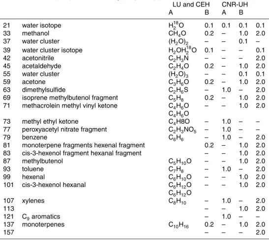
Table 1. PTR-MS measurement cycles, the compounds contributing to the measured masses, and the PTR-MS integration, or dwell, times. For LU and CEH the cycle length was 1.4 s in the micrometeorological flux measurements (A) and 7.1 s in the ambient mixing ratio measurements (B). For CNR-UH the cycle lengths were 13.3 and 37.5 s, respectively.

Protonated mass [amu] and contributing compound(s) Formula Dwell time [s]

LU and CEH CNR-UH

A B A B

21 water isotope H18₂ O 0.1 0.1 0.1 0.1

33 methanol CH4O 0.2 – 1.0 2.0

37 water cluster (H₂O)₂ – – 0.1 –

39 water cluster isotope H₂OH18₂ O 0.1 – – 0.1

42 acetonitrile C2H3N – – – 2.0

45 acetaldehyde C2H4O 0.2 – 1.0 2.0

55 water cluster (H2O)3 – – 0.1 0.1

59 acetone C3H6O 0.2 – 1.0 2.0

63 dimethylsulfide C2H6S – 1.0 – 2.0

69 isoprene methylbutenol fragment C₅H₈ 0.2 – 1.0 2.0

71 methacrolein methyl vinyl ketone C₄H₆O – – 1.0 2.0

C4H6O

73 methyl ethyl ketone C4H8O – 1.0 – –

77 peroxyacetyl nitrate fragment C2H3NO5 – 1.0 – –

79 benzene C6H6 – 1.0 – 2.0

81 monoterpene fragments hexenal fragment 0.2 – 1.0 2.0

83 cis-3-hexenol fragment hexanal fragment – – 1.0 2.0

87 methylbutenol C₅H₁₀O – – 1.0 2.0

93 toluene C7H8 – 1.0 – 2.0

99 hexenal C6H10O – – 1.0 2.0

101 cis-3-hexenol hexanal C6H12O – – 1.0 2.0

C6H12O

107 xylenes C8H10 – 1.0 – 2.0

113 – – 1.0 2.0

121 C₉aromatics – 1.0 – –

137 monoterpenes C₁₀H₁₆ 0.2 – 1.0 2.0

(28)

BGD

6, 2183–2216, 2009

B. Davison et al.

Title Page

Tables Figures

◭ ◮

Back Close

Full Screen / Esc

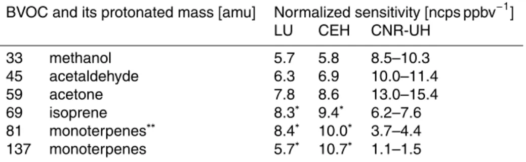
Table 2. Normalized sensitivities for the BVOCs presented in this paper. The PTR-MS in-struments of LU and CEH were calibrated twice (on 6 and 13 May 2007) and the PTR-MS of CNR-UH was calibrated three times during the second part of the campaign (on 20, 25, and 31 May).

BVOC and its protonated mass [amu] Normalized sensitivity [ncps ppbv−1

] LU CEH CNR-UH

33 methanol 5.7 5.8 8.5–10.3

45 acetaldehyde 6.3 6.9 10.0–11.4

59 acetone 7.8 8.6 13.0–15.4

69 isoprene 8.3∗ 9.4∗ 6.2–7.6

81 monoterpenes∗∗ 8.4∗ 10.0∗ 3.7–4.4 137 monoterpenes 5.7∗ 10.7∗ 1.1–1.5

∗ _{These values were not measured but calculated using proton transfer reaction rate coe} ffi -cients and transmission coefficients.

(29)

BGD

6, 2183–2216, 2009

B. Davison et al.

Title Page

Tables Figures

◭ ◮

Back Close

Full Screen / Esc

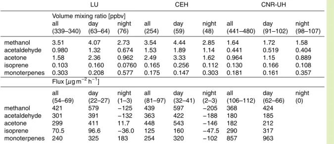
Table 3. Medians of BVOC mixing ratios and fluxes calculated from all, daytime (12:00– 17:00 LT), and night-time (00:00–05:00 LT) measurements. The measurement period was 7–14 May 2007 for LU and CEH and 20 May–3 June 2007 for CNR-UH. The number of measure-ments contributing to the median is given in parentheses.

LU CEH CNR-UH

Volume mixing ratio [ppbv]

all day night all day night all day night

(339–340) (63–64) (76) (254) (59) (48) (441–480) (91–102) (98–107)

methanol 3.51 4.07 2.73 3.54 4.44 2.85 1.64 1.72 1.58

acetaldehyde 0.980 1.32 0.674 1.53 1.89 1.14 0.441 0.519 0.404

acetone 1.58 2.36 0.962 2.49 3.33 1.62 0.964 1.15 0.889

isoprene 0.103 0.160 0.0760 0.165 0.256 0.112 0.130 0.166 0.108

monoterpenes 0.303 0.208 0.577 0.175 0.147 0.303 0.181 0.161 0.357

Flux [µg m−2

h−1

]

all day night all day night all day night

(54–69) (22–27) (1–3) (81–97) (32–41) (2–3) (106–112) (62–66) (0)

methanol 421 579 −125 439 597 −205 368 424

acetaldehyde 301 391 −132 363 422 −188 180 185

acetone 299 411 11.7 448 543 −146 182 212

isoprene 70.5 96.6 −36.0 125 160 −47.5 290 317

(30)

BGD

6, 2183–2216, 2009

B. Davison et al.

Title Page

Tables Figures

◭ ◮

Back Close

Full Screen / Esc

(31)

BGD

6, 2183–2216, 2009

B. Davison et al.

Title Page

Tables Figures

◭ ◮

Back Close

Full Screen / Esc

(32)

BGD

6, 2183–2216, 2009

B. Davison et al.

Title Page

Tables Figures

◭ ◮

Back Close

Full Screen / Esc

(33)

BGD

6, 2183–2216, 2009

B. Davison et al.

Title Page

Tables Figures

◭ ◮

Back Close

Full Screen / Esc

(34)

BGD

6, 2183–2216, 2009

B. Davison et al.

Title Page

Tables Figures

◭ ◮

Back Close

Full Screen / Esc