www.atmos-chem-phys.net/11/4121/2011/ doi:10.5194/acp-11-4121-2011
© Author(s) 2011. CC Attribution 3.0 License.
Chemistry
and Physics
The influence of small-scale variations in isoprene concentrations on
atmospheric chemistry over a tropical rainforest
T. A. M. Pugh1, A. R. MacKenzie1, B. Langford1,*, E. Nemitz2, P. K. Misztal2,3,**, and C. N. Hewitt1
1Lancaster Environment Centre, Lancaster University, Lancaster, UK 2Centre for Ecology and Hydrology, Edinburgh, UK
3School of Chemistry, University of Edinburgh, Edinburgh, UK *now at: Centre for Ecology and Hydrology, Edinburgh, UK
**now at: Department of Environmental Science, Policy, and Management, University of California, Berkeley, CA, USA Received: 16 April 2010 – Published in Atmos. Chem. Phys. Discuss.: 30 July 2010
Revised: 12 April 2011 – Accepted: 29 April 2011 – Published: 4 May 2011
Abstract. Biogenic volatile organic compounds (BVOCs) such as isoprene constitute a large proportion of the global atmospheric oxidant sink. Their reactions in the atmosphere contribute to processes such as ozone production and sec-ondary organic aerosol formation. However, over the tropi-cal rainforest, where 50 % of the global emissions of BVOCs are believed to occur, atmospheric chemistry models have been unable to simulate concurrently the measured daytime concentration of isoprene and that of its principal oxidant, hydroxyl (OH). One reason for this model-measurement dis-crepancy may be incomplete mixing of isoprene within the convective boundary layer, leading to patchiness or segre-gation in isoprene and OH mixing ratios and average con-centrations that appear to be incompatible with each other. One way of capturing this effect in models of atmospheric chemistry is to use a reduced effective rate constant for their reaction. Recent studies comparing atmospheric chemistry global/box models with field measurements have suggested that this effective rate reduction may be as large as 50 %; which is at the upper limit of that calculated using large eddy simulation models. To date there has only been one field campaign worldwide that has reported co-located measure-ments of isoprene and OH at the necessary temporal resolu-tion to calculate the segregaresolu-tion of these compounds. How-ever many campaigns have recorded sufficiently high resolu-tion isoprene measurements to capture the small-scale fluctu-ations in its concentration. Assuming uniform distributions
Correspondence to:T. A. M. Pugh ([email protected])
of other OH production and loss processes, we use a box model of atmospheric chemistry, constrained by the spec-trum of isoprene concentrations measured, as a virtual in-strument, to estimate the variability in OH at a point and hence, to estimate the segregation intensity of isoprene and OH from high-frequency isoprene time series. The method successfully reproduces the only directly observed segrega-tion, using measurements made in a deciduous forest in Ger-many. The effective rate constant reduction for the reaction of isoprene and OH over a South-East Asian rainforest is calculated to be typically<15 %. Although there are many unconstrained uncertainties, the likely nature of those pro-cesses suggests that this value represents an upper limit. The estimate is not sensitive to heterogeneities in NO at this re-mote site, unless they are correlated with those of isoprene, or to OH-recycling schemes in the isoprene oxidation mech-anism, unless the recycling happens in the first reaction step. Segregation alone is therefore unlikely to be the sole cause of model-measurement discrepancies for isoprene and OH above a rainforest.
1 Introduction
emissions of isoprene occur, for instance the tropical rain-forest or mid-latitude deciduous rain-forests, should see suppres-sion of hydroxyl radical (OH) concentrations in the bound-ary layer (Wang et al., 1998; Lawrence et al., 1999; Granier et al., 2000; Poisson et al., 2000; Lelieveld et al., 2002; von Kuhlmann et al., 2004; J¨ockel et al., 2006). This is of great consequence, as the OH radical is the primary sink for a large range of chemicals emitted into the atmosphere, including the greenhouse gas methane.
Over the past decade several measurement studies have noted much higher concentrations of OH in areas of high iso-prene concentration than has been predicted by models of at-mospheric chemistry (Tan et al., 2001; Carslaw et al., 2001; Ren et al., 2008; Lelieveld et al., 2008; Martinez et al., 2010; Hofzumahaus et al., 2009; Pugh et al., 2010). It has been proposed that the sources of OH in these high isoprene envi-ronments may be underestimated and several suggestions for additional methods of OH formation have been put forward (Lelieveld et al., 2008; Hofzumahaus et al., 2009; Peeters et al., 2009; Whalley et al., 2011). Whilst these methods are successful in increasing modelled [OH]1in these regions to within the bounds of the measurements, these increases in [OH] lead to faster oxidation, and hence lower concentra-tions, of isoprene. Butler et al. (2008) and Pugh et al. (2010) have shown that the increases in isoprene emission required to rectify this isoprene underestimation exceed the available isoprene flux in these regions and furthermore lead to a re-suppression of [OH].
Butler et al. (2008) hypothesised that the reason for the discrepancy between modelled and measured isoprene and OH may lie with the rate of reaction between isoprene and OH used in chemical models. The rate of change of isoprene concentration with respect to its reaction with OH can be rep-resented by
∂hC5H8i
∂t = −kC5H8,OH(hOHihC5H8i + hOH
′C5H8′i), (1)
where the angle brackets represent volume averages, and the primes represent deviations from the mean concentration. In a typical atmospheric chemistry model, concentrations are assumed to be uniform within a box and the term containing the primes is neglected. However studies with large eddy simulation (LES) models have shown that the contribution of the prime term can be substantial for atmospheric reactions where the timescale of the chemical reaction is of the same order as the mixing timescale (e.g. Schumann, 1989; Sykes et al., 1994; Krol et al., 2000; Patton et al., 2001; Vinuesa and Vil`a Guerau de Arellano, 2003). Using an intensity of segregation metric,S(e.g. Krol et al., 2000), where
SC5H8,OH=
hOH′C5H8′i
hOHihC5H8i, (2)
1Square brackets are used herein to indicate concentrations
where no averaging has been applied or is specified.
this effect can be represented by a modified reaction rate co-efficient,keff,
keff=kC5H8,OH(1+SC5H8,OH). (3)
A negative value of S implies that the two reactants are spatially anti-correlated, whereas a positive value implies a positive correlation, and S= 0 indicates a random dis-tribution of anomalies or a homogeneous disdis-tribution. In their idealised LES modelling study, Krol et al. (2000) found that, under conditions of heterogeneous emissions,
SVOC,OH=−0.294 was simulated for a reaction between a VOC and OH. In their study, the effective reaction rate of VOC and OH was 25 % of that of the C5H8+ OH reaction rate at 298K (IUPAC, 2009). Similarly, in the development of a parameterisation for segregation intensity, Vinuesa and Vil`a Guerau de Arellano (2005) suggestSVOC,OH= -0.405, where the reactants react at a rate similar to that of the C5H8 + OH reaction rate at 298 K. Such segregation can occur for C5H8and OH because, due to the extremely rapid reaction rate between the two compounds, [OH] rapidly approaches a steady state between its loss due to isoprene and its var-ious production processes, on a timescale of the order of one second (Appendix A). Therefore if isoprene is not uni-formly distributed throughout the model box, OH concentra-tions will also vary, with the lowest OH concentraconcentra-tions co-located with the highest isoprene concentrations, assuming other OH sinks are uniform. Isoprene itself has a chemical lifetime in the boundary layer which is similar to typical tur-bulent mixing timescales (e.g. Butler et al., 2008; Pugh et al., 2010), while its flux into the BL is subject to heterogeneities likely influenced by the coupling of the canopy to the tur-bulent BL (e.g. Patton et al., 2001), the local dispersion of isoprene emitting plants, and variations in light and temper-ature. Therefore it is highly probable that heterogeneities of isoprene concentration within the boundary layer will occur. Based upon comparisons between measurements over the Amazonian rainforest and simulations using a global chem-istry model, Butler et al. (2008) foundSC5H8,OH=−0.6 was
required to reconcile measured and modelled concentrations if the standard IUPAC rate constant for C5H8+ OH is used.2 In a similar experiment, but using a box model and measure-ments over a south-east Asian rainforest as part of the Oxi-dant Particle and Photochemical Processes (OP3) campaign, Pugh et al. (2010) requiredSC5H8,OH=−0.5 to attain a good
agreement between measurements and their model. Consid-ering that there is also a 20 % uncertainty in the IUPAC rate constant, such values do not appear unreasonable in the con-text of the LES studies above.
Direct atmospheric measurements of segregation require co-located measurements of both species at a temporal res-olution fast enough to resolve the smallest relevant spatial 2Butler et al. (2008) report a rate constant reduction of 50 %
below the lower uncertainty bound of the C5H8+ OH rate constant
scales. Butler et al. (2008) calculatedSC5H8,OH=−0.13
us-ing aircraft measurements over the Guyanas; however at the speed of the aircraft the temporal resolution of the measure-ments resulted in a measurement scale of the order of several hundred metres. Hence smaller scale segregation would have been missed. To date only one study has measuredSC5H8,OH
at a ground-based station, with Dlugi et al. (2010) finding values ofSC5H8,OH as negative as−0.15 over a deciduous
forest in Germany, although their study is limited to a single day of measurements.
During OP3, high-temporal resolution measurements of [OH] co-located with those of isoprene were not available. Here we use high temporal resolution isoprene concentration measurements (Langford et al., 2010) made over a south-east Asian rainforest as part of the OP3 campaign (Hewitt et al., 2010), in conjunction with a box model of atmospheric chemistry, which is used as a virtual instrument to estimate [OH], and hence estimate the intensity of segregation of iso-prene and OH in this region. First the measurements are de-scribed, followed by a description of the modelling approach used. Results are then presented and discussed.
2 Measurements
Measurements of isoprene concentration were made using a proton-transfer reaction mass spectrometer (PTR-MS) dur-ing April/May 2008 at the Bukit Atur Global Atmosphere Watch station (4◦ 58′59′′N, 117◦ 50′39′′E ). The station is located at an altitude of 437 m a.m.s.l., on a small hill approx-imately 260 m above the valley floor and the surrounded by primary and secondary rainforest (Hewitt et al., 2010), with a typical canopy height of 25 m (N. Chappell, Lancaster Uni-versity, pers. comm.). On top of the hill stands a 100 m tall, open-pylon type tower which was instrumented with a sonic anemometer at 75 m and a low pressure (60 kPa) PTFE gas inlet tube (length: 85 m; OD 12′′). For the purpose of tur-bulence calculations, these measurements are considered to be∼125 m above the forest canopy, taking into account that the measurement tower is sited on a hill (Helfter et al., 2010; Langford et al., 2010).
The PTR-MS was housed in an air-conditioned laboratory at the base of the tower and sub-sampled from the inlet at a rate of 0.3 lmin−1, via a short length of PTFE tubing (18′′ OD). The flow in the main inlet line was turbulent, minimis-ing the dampenminimis-ing of the VOC signal (Spirig et al., 2005). Individual compounds were sampled, iteratively, providing for each compound a disjunct time-series with a value every
∼7 s, that is measured with an integration time of 0.5 s and an overall instrument response time of 1 s. These data are avail-able for a continuous 25 min period out of every 30 min. The remaining 5 min were devoted to calibration techniques and scans of the mass spectrum. A complete description of these measurements and set-up can be found in Langford et al. (2010).
8 10 12 14 16 18 20 22 24
0 1 2 3 4 5 6 7 8
Hour of day (decimal) C5
H8
mixing ratio (ppbv)
14.252 14.3 14.35 14.4 14.45 14.5
3 4 5 6
Fig. 1. Isoprene concentration data measured by PTR-MS for 26/04/08 showing 1 data point every 10 s. The inset shows a 15 min extract (note hours given as decimal fraction) indicating the short timescale over which large variations can occur.
Figure 1 shows an example of isoprene concentration mea-surements for a single day (26 April 2008). Although the diurnal cycle in the measurements is clear, substantial varia-tion is seen around the mean. The inset indicates that these variations in isoprene concentration often have a magnitude similar to the mean isoprene concentration. These fluctua-tions occur on a timescale of less than one minute. If they are characteristic of the real atmosphere they indicate large inhomogeneities in the isoprene distribution on length scales of<180 m, considering a wind speed<3 ms−1.
To test whether these concentration fluctuations are a real feature of the atmosphere, or are due to instrument noise, a statistical analysis was carried out. Hayward et al. (2002) showed that the instrument noise signal for the PTR-MS can be well-approximated by a Gaussian distribution. They show that the standard deviation of noise varies with the signal strength and can be reliably predicted by the noise statistic (NS):
NS=√c
c×δ, (4)
wherecis the mean signal recorded by the PTR-MS in units of ion counts per second, i.e. the number of instances in which that compound is registered at the detector each sec-ond. This is later converted into a mixing ratio as described in Langford et al. (2010). The dwell time,δ, is the time spent scanning for each compound. For more information on these terms the reader is referred to Hayward et al. (2002). AsNS is analogous to standard deviation, if the rapid fluctuations in the measured isoprene concentration are purely due to in-strument noise, 4.4 % of recorded values should fall outside
1 1.5 2 2.5 3 3.5 4 4.5 0
0.1 0.2 0.3 0.4 0.5 0.6 0.7
C5H8 mixing ratio (ppbv)
Probability density
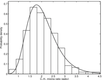
Fig. 2. Histogram showing distribution of isoprene concentrations between 11:00 and 12:00 LT on 30 April 2008. The line shows the probability density function for a log-normal distribution.
Calculating NS for the isoprene concentration data col-lected between 10:00–18:00 LT on 26 April 2008, using a 10 min running mean to calculatec, reveals that 10.5 % of these data lie outside ±2NS (3000 datapoints). This indi-cates that instrument noise is highly unlikely to be responsi-ble for all of the variation measured and shows that variations in isoprene concentration of this magnitude were present in the atmosphere during OP3. In addition, the distribution is close to log-normal (Fig. 2), which is representative of the statistical distribution of atmospheric concentrations, rather than random ion noise, which follows a Poisson distribu-tion. Although it is not possible to differentiate between the smaller variations and instrument noise, it is the large fluc-tuations that will be of most importance in the analysis that follows.
3 Modelling
3.1 Approach
If a snapshot of the boundary layer is taken in time, a range of isoprene concentrations will be revealed in the spatial do-main. Because isoprene is the dominant OH sink in the trop-ical forest environment, the variability in isoprene concen-tration induces variability in OH concenconcen-tration. If isoprene is well mixed within the boundary layer, the variations in isoprene (and thus OH) concentrations will be small, and av-erage concentrations are sufficient for calculations of chem-istry. However, a boundary layer in which isoprene is not well mixed will display a large standard deviation of concen-trations for isoprene, which will induce a large variation in OH concentrations, resulting in a strong covariance between isoprene and OH. Ideally co-located measurements would be
used to measure this covariance. However, here we argue that the OH time series that would have resulted from a suitable OH measurement co-located with the isoprene measurement, can be estimated purely on the basis of chemistry. For most species such a procedure would not be possible. However, two key simplifying aspects of our system are (a) that OH is produced in-situ everywhere throughout the boundary layer and, (b) due to its short lifetime, OH is always in steady-state with its chemical sources and sinks. This means that the OH concentration at a place and time is independent of the history of the air at that place. The OH concentration is therefore a function of the instantaneous value of chemi-cal production,P, its major chemical sink in the rainforest environment, isoprene, and other chemical sinks,OL:
[OH] =f ([C5H8],P ,OL), (5)
and there are no advective terms to be considered. Our knowledge of (and uncertainty in) the chemical source and sink terms for OH is embodied in chemical mechanisms. It follows that our best theoretical estimate of OH mixing ratios will come from integrating chemical mechanisms to steady-state, given adequate empirical data on the mixing ratios of longer-lived compounds that dominateP andOL.
The ratio of turbulent timescale to chemical timescale is known as the Damk¨ohler ratio (Da). Turbulence and
chem-istry interact whenDais of the order of 1. ForDa≪1 turbu-lence controls the variability and forDa≫1 chemistry
dom-inates (Vil`a Guerau de Arellano et al., 1995). The OH life-time, with respect to isoprene, at a typical mixing ratio of 2 ppbv, is 0.22 s at 298 K. The median diurnal profile of verti-cal velocity during the OP3 measurement period considered in this paper peaks at approximately 0.2 m s−1. Therefore the transport distance of OH during its lifetime is less than 0.05 m, cf. the scale of a few metres we assume for our mea-sured air parcels (based upon a typical windspeed of a few metres per second and Taylor’s frozen turbulence hypothe-sis, Powell and Elderkin, 1974), and thereforeDa≫1. As
a result any covariance of isoprene and OH must be due to the OH concentration adjusting chemically to a change in the isoprene concentration, demonstrating requirement (b). Dlugi et al. (2010) also found transport of OH to be negligi-ble based on both the same logic, and on measurements of OH fluxes.
In order to fully captureSC5H8,OHisoprene must be
utilising a LES model, Vinuesa and Porte-Agel (2008) found that the sub-grid scale mixing term could be neglected when a horizontal resolution of∼50 m or less was used. In our study, at the high effective measurement height of 125 m,
>90 % of the variance and flux were estimated to be carried in eddies slower than 1 Hz (Helfter et al., 2010; Langford et al., 2010) and it is likely that the high-frequency contribu-tion to the OH-isoprene covariance is even smaller because of the damping induced by the fast chemistry. Thus the isoprene measurement is thought to be taken at a sufficiently high tem-poral resolution to effectively characteriseSC5H8,OH.
If, in addition, the air advecting past the measurement point is assumed to contain a range of isoprene concentra-tions representative of the boundary layer as a whole, then the measurements can be generalised to the whole boundary layer for comparison with results from atmospheric chem-istry models. The close agreement found between the aver-age of the isoprene measurements used in this study and air-craft measurements made in the boundary layer (Hewitt et al., 2009) gives confidence that the PTR-MS isoprene measure-ments used here are representative of the boundary layer as a whole, fufilling this condition.
Because the isoprene measurement is non-continuous, it only provides a good statistical representation of the distribu-tion of 1 s data points. Some of the informadistribu-tion on the tempo-rally organised structure in the variability does get lost. How-ever, as discussed above, the OH concentration at a place and time is independent of the history of the air at that place. Therefore, given a sufficient time window,ts, a
representa-tive sample of the population of isoprene concentrations ad-vected past the detector should be obtained, and a histogram can be constructed showing the probability distribution of the measured isoprene concentration (Fig. 2).
By calculating the average sampled isoprene concentra-tion and modelled OH concentraconcentra-tion overts, estimates can
be gained forhC5H8iandhOHi. Hence Eq. (2) can be ap-proximated by,
SC5H8,OH≈
OH′C5H8′
OHC5H8 , (6)
where the over-bars represent time averages. We are not di-rectly converting a time series measurement into a spatial scale of eddy size (evoking Taylor’s frozen turbulence hy-pothesis). Rather a set of discreet samples recorded in the time domain are used to represent the spatial variation of a population of those samples throughout the boundary layer. An appropriate length fortsis discussed in Sect. 3.2. We note
that this method is not a direct measurement ofSC5H8,OH in
the BL. However, given the complexities of making such a direct measurement, this approximation is of utility.
Because, as explained previously, transport of OH is neg-ligible, the OH concentration at a point in space and time can
be calculated from all the production and loss terms at that point by expanding Eq. (5),
[OH]= P
(kC5H8,OH[C5H8])+(kOL,OH[OL])
. (7)
WhereOLis the sum of all OH sinks other than C5H8, and
P is the OH production rate. Our approximation (discussed further below) is that the species determiningP andOLare well-mixed compared to isoprene. Hence, when computing OH at the point in space and time at which the isoprene mea-surements are made, we use the instantaneous value of iso-prene but volume average values forP andOLderived from the box model. We discuss the implications of our approxi-mations for the calculation ofSC5H8,OHin Sect. 4.3 and
con-clude that our value for the magnitude ofSC5H8,OH is likely
to be an upper limit.
AsP andOL are complicated terms, they are most eas-ily calculated using a numerical chemistry box model con-strained to the measured [C5H8]. It is emphasised here that the box model is used purely as a convenient tool to carry out chemical mechanism calculations, and not to capture mixing processes. Hence the chemical model acts as a virtual OH instrument with precisely the temporal and spatial resolution of the isoprene measurements. Note that this method does not produce a continuous [OH] time-series, but rather a set of [OH] samples, which correspond to the measured samples of [C5H8] at a given time. If the re-equilibration of OH con-centrations (Appendix A) occurred over a longer time period than the isoprene sampling interval, then the model would not find the new steady-state [OH] before the next change in [C5H8], and the model generated [OH] time-series would not be valid, given that no information exist on the isoprene con-centration of 9 s after each 1 s sample. Appropriate values for [OH] and [C5H8] are provided by taking running means over the time window,ts. So effectively a running sample of
the population is being taken. This avoids unnecessary and arbitary discretisation of the segregation signal and is simi-lar to running mean filtering in the calculation of surface ex-change fluxes, i.e. co-variances of concentration with wind components (McMillen, 1988). OH′and C5H8′are then eas-ily calculated from the time series, and henceSC5H8,OH can
be calculated using Eq. (6).
An important consideration are the secondary oxidation products of isoprene, which may be preferentially co-located with high isoprene concentrations, depending on the ratio of the turbulence timescale, τt, to their chemical lifetime,τc.
However, the lifetimes of all secondary oxidation products of isoprene which may impact the OH sink are much greater than the timescale for mixing out of our measured air parcel, which has a length-scale of a few metres (Da≪1). Hence it is
assumed that the concentrations of secondary oxidation prod-ucts of isoprene are not co-variant with those of isoprene, and effectively consistute random noise in theSC5H8,OH signal.
only. The use of the constrained box model in the manner described above implicitly mixes all species homogeneously across all air samples if those species have a lifetime longer than the sampling period. It is worth noting here that the ac-curacy of this method is greatly increased if the OH sink is dominated by isoprene chemistry (as at both sites in Sect. 4), as this reduces potential errors due to a possible poor charac-terisation ofOL.
Running a model constrained to measured concentrations is a typical approach for studying chemical processes in the atmosphere and testing model chemical mechanisms us-ing both ground-based (e.g. Carslaw et al., 2001; Emmer-son et al., 2005, 2007; Hofzumahaus et al., 2009; Kanaya et al., 2007, 2009) and aircraft-based (e.g. Ren et al., 2008; Kubistin et al., 2010) measurements. However a model has not before been used in this manner as a virtual instrument, for the purposes of calculating segregation. The above listed studies typically use measurements of VOCs, NOx, O3, CO and other intermediate/long-lived species, as boundary con-ditions to attempt to calculate radical concentrations. All these studies utilise measurements with a temporal resolution of greater than 1 min for the aircraft based measurements and in the region 5–15 min for the ground based measurements. They are all therefore likely to miss much of the fine-scale segregation of species investigated in this work. We em-phasise that the constrained method is only appropriate for calculating covariances when the frequency of the measure-ments is high and the modelled species is not significantly transported.
3.2 Model setup
The CiTTyCAT box model of atmospheric chemistry (Wild et al., 1996; Evans et al., 2000; Emmerson et al., 2004; Dono-van et al., 2005; Real et al., 2007, 2008; Hewitt et al., 2009; Pugh et al., 2010) is used to apply this approach to the OP3 measurements. The model is run for the 12 h of daylight be-tween 06:00 and 18:00 LT, and isoprene concentration is con-strained by each of the 1 s measured concentrations, run for 10 s. Gaps in the isoprene time series are filled by replicating a section of the immediately preceding data the same length as the gap. This is deemed acceptable as the characteristic spectrum of isoprene timescales is what is of interest in this analysis. If the 12 h data period contains gaps greater than 30 min, data for that day are discarded. In total eleven days of suitable data are available for analysis for the first OP3 campaign (OP3-1) (April–May 2008).
The model is integrated on a time step of 1s, although the chemical solver itself uses intermediate time steps of a variable size (Brown et al., 1989). As the model has pre-viously been optimised for the OP3 scenario by Pugh et al. (2010), the set-up described in that paper is largely retained, with the model being fed campaign average values of cloud cover (calculated usingj (O1D)as a proxy) and temperature. Boundary layer height is set to 800 m throughout the run.
6 8 10 12 14 16 18 −0.25
−0.2 −0.15 −0.1 −0.05 0
Hour of day
SC5H8,OH
ts = 10 min ts = 30 min ts = 60 min ts = 120 min
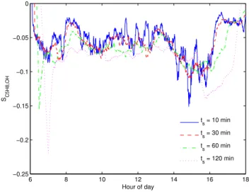
Fig. 3. Variation in SC5H8,OH due to using ts= 10, 30, 60 and
120 min. Carried out using OP3 isoprene measurements collected on 30/04/08.
However it must be cautioned that LIDAR measurements of boundary layer height (Pearson et al., 2010) indicate that the BL is well-mixed throughout this 800 m range only be-tween the hours of 10:00–18:00 LT. Therefore results before 10:00 LT will not be representative of the BL as a whole. In-deed the first hour must be discarded as spin-up time. We emphasise here that the BL height is only used for scaling the deposition rates of various intermediate species and the emission rate of NO, which both play some role in the calcu-lation of the bulk termsP andOL(see Eq. 7). The influence of the chosen BL height on isoprene-OH covariances is indi-rect and minor.
Finally, the length of the time window, ts, is of
impor-tance. When selecting ts it must be considered what
ele-ments should be classified as segregation and at what time-scale variations start to reflect changing conditions (non-stationarities). For instance, if ts= 1 h, then variations in
cloud cover and solar zenith angle may make a significant contribution to the variation. However, cloud cover and solar zenith angle changes are typically uniform across the bound-ary layer and therefore do not contribute to the spatial vari-ation which is the subject of this work. In order to ensure that only factors such as canopy emission and BL turbulence dominate the variation, a shorterts is required. To determine
how short, the fast Fourier transform of measuredj(O1D) (which implicitly incorporates both cloud cover and solar zenith angle changes) is computed (not shown); this indicates little variation on timescales shorter than 10 min, suggesting
ts= 10 min would be sufficiently small to eliminate the effect
be appropriate for their measurements of segregation inten-sity over a forest in Germany, by examining the covariances of OH and j(O1D). As usingts= 10 min also ignores the
ef-fects of slower frequency eddies, test calculations forts= 10,
30, 60 and 120 min have been computed to give an indication of how the result is affected. Calculations were carried out using isoprene measurements collecting during the OP3 cam-paign on 30 April 2008. Figure 3 shows that the greatest de-viations occur at the ends of the day, when changes in j(O1D)
are most rapid. Even when usingts= 120 min, which clearly
incorporates significant non-stationarities, results during the middle period of the day were generally within a factor of two of those generated usingts= 10 min.
4 Results and discussion
4.1 Case study of OH-isoprene interactions above a German mixed forest (Dlugi et al., 2010)
Dlugi et al. (2010) appear to have provided the only clear observations ofSC5H8,OH to date. Therefore, to test the
ap-proach described above before making calculations for the OP3 campaign, the model was run for 4 h between 10:00 and 14:00 LT using an isoprene concentration time series pro-duced by generating random numbers according to the dis-tribution statistics specified in Dlugi et al. (2010). As only limited information about the physical and chemical char-acteristics of the Dlugi et al. (2010) measurement site were available, the model setup used for OP3 was retained with the following exceptions: The box was positioned at 50◦54′N, 6◦24′E, with NO emissions from the Yienger and Levy (1995) inventory for that location being used. The j(O1D)
measurements reported in Dlugi et al. (2010) were approxi-mated by modifying the model cloud cover and the reported temperature measurements were also used. Initial concentra-tions for O3, NO, HCHO, MACR, MVK and HONO were set as reported in Dlugi et al. (2010) and Kleffmann et al. (2005), the latter measurements were for the same site but they were made a month earlier. As CiTTyCAT is currently unable to replicate the magnitude of daytime HONO forma-tion that was observed at this site, the model is constrained to a constant HONO mixing ratio of 150 pptv, following the measurements of Kleffmann et al. (2005).
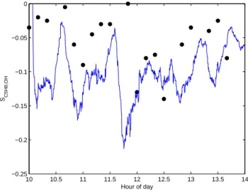
The result of this test is shown in Fig. 4. A reasonable agreement is achieved in terms of the timing and magni-tude of the main peaks. The model does not capture all the variability in the observed data and tends to overesti-mate the depth of the troughs. However, as will be discussed in Sect. 4.3, the concentration of OH sinks other than iso-prene has a damping effect on the magnitude ofSC5H8,OH.
At a site such as this in Western Europe, the concentrations of background species contributing to the OH sink may be quite high. Hence it is likely that our model will somewhat overestimate the magnitude ofSC5H8,OHin this case, without
10 10.5 11 11.5 12 12.5 13 13.5 14
−0.25 −0.2 −0.15 −0.1 −0.05 0
Hour of day
SC5H8,OH
Fig. 4.Comparison of the observedSC5H8,OHof Dlugi et al. (2010) (black dots), with the model estimate using the approach described in this paper (ts=10 min) (blue line).
detailed information for the background species. When the distributions of SC5H8,OH from Dlugi et al. (2010) and our
model are normalised to a mean of zero, a Kolomogorov-Smirnov test indicates that they are both from the same dis-tribution at the 99 % confidence level. This suggests that the variability ofSC5H8,OHis well represented by this modelling
approach. Overall the agreement achieved is encouraging, suggesting that the model can effectively estimateSC5H8,OH
from the supplied isoprene data.
4.2 Application to a tropical forest (OP3)
Figure 5 shows the intensity of segregation calculated by the model for each day of available data for the OP3 cam-paign. SC5H8,OHis much less negative than suggested in the
studies of Butler et al. (2008) and Pugh et al. (2010) with a 10:00–18:00 LT mean ofSC5H8,OH=−0.054 forts= 10 min,
resulting in keff being 5.4 % smaller thankC5H8,OH. When
ts= 60 min, the 10:00–18:00 LT mean ofSC5H8,OH=−0.068,
resulting in keff being 6.8 % smaller than kC5H8,OH.
Fig-ure 6 shows that the distribution ofSC5H8,OH during
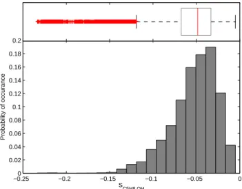
OP3-1 is strongly skewed with a tail towards the more nega-tive values, with the median slightly less neganega-tive than the mean atSC5H8,OH=−0.049 forts= 10 min. The 5th and 95th
percentiles areSC5H8,OH=−0.104 andSC5H8,OH= -0.018
re-spectively. A large variation inSC5H8,OH is modelled over
the course of each day, but 10 min average values never fall belowSC5H8,OH=−0.25. GenerallySC5H8,OH computed
us-ingts= 60 min is more negative than forts= 10 min, however
the difference is not pronounced, with major deviations only occurring on a few occasions. This suggests that the most important component ofSC5H8,OH is that due to turbulence
6 8 10 12 14 16 18 −0.25
−0.2 −0.15 −0.1 −0.05 0
21/04/08
SC5H8,OH
6 8 10 12 14 16 18
−0.25 −0.2 −0.15 −0.1 −0.05 0
22/04/08
6 8 10 12 14 16 18
−0.25 −0.2 −0.15 −0.1 −0.05 0
23/04/08
6 8 10 12 14 16 18
−0.25 −0.2 −0.15 −0.1 −0.05 0
24/04/08
SC5H8,OH
6 8 10 12 14 16 18
−0.25 −0.2 −0.15 −0.1 −0.05 0
25/04/08
6 8 10 12 14 16 18
−0.25 −0.2 −0.15 −0.1 −0.05 0
29/04/08
SC5H8,OH
6 8 10 12 14 16 18
−0.25 −0.2 −0.15 −0.1 −0.05 0
27/04/08
6 8 10 12 14 16 18
−0.25 −0.2 −0.15 −0.1 −0.05 0
30/04/08
6 8 10 12 14 16 18
−0.25 −0.2 −0.15 −0.1 −0.05 0
01/05/08
6 8 10 12 14 16 18
−0.25 −0.2 −0.15 −0.1 −0.05 0
02/05/08
Hour of day SC5H8,OH
6 8 10 12 14 16 18
−0.25 −0.2 −0.15 −0.1 −0.05 0
03/05/08
Hour of day
6 8 10 12 14 16 18
−0.25 −0.2 −0.15 −0.1 −0.05 0
Hour of day Mean
Fig. 5. Model calculated intensity of segregation forts= 10 min, showing each day during OP3-1 and the overall mean. Note that results
before 10:00 LT are not representative of the boundary layer as a whole.
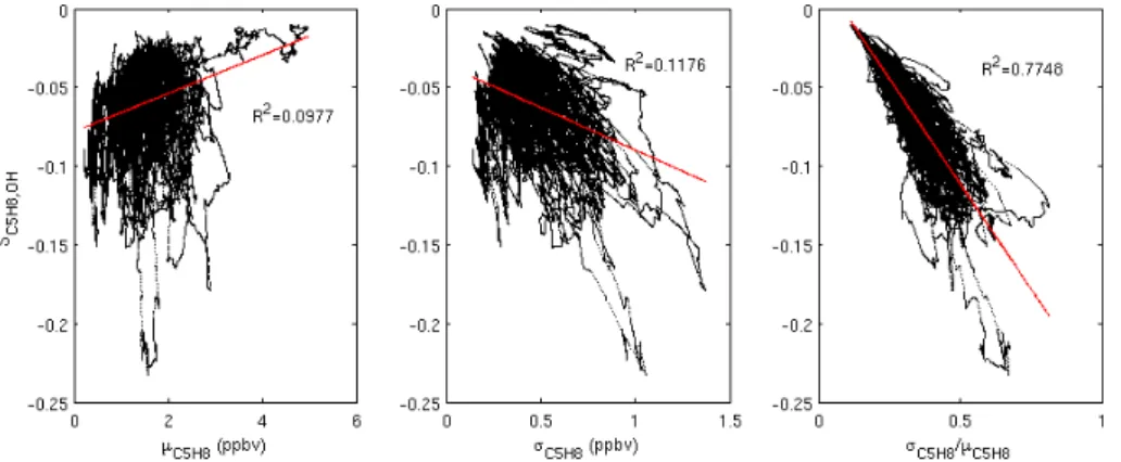
Figure 7 shows thatSC5H8,OH is not strongly correlated
with either the standard deviation (σ) or the mean (µ) of the isoprene concentration. However the combination of these two statistics, σC5H8/µC5H8, i.e. the relative standard
deviation, correlates strongly with the intensity of segrega-tion. This is likely due to the rate of increase of the overall reaction rate of isoprene and OH,dRC5H8,OH/hC5H8i,
de-creasing with inde-creasing isoprene concentration. Therefore a givenσC5H8 will produce a greater range ofRC5H8,OH over
ts, whenµC5H8 is low. This indicator becomes less accurate
asSC5H8,OHbecomes more negative; we can find no simple
explanation for this increase in scatter. It could be due to a combination of the skewness and kurtosis of the isoprene distribution, combined with the OH production rate and the size of the non-isoprene OH sink. One feature of the plots in Fig. 7 is that, rather than a quasi-random scatter of data, the
data points tend to arrange themselves in trajectories. This is most obvious with some of the outliers. This behaviour is a result of using running means over the input data, meaning that each point is influenced to some extent by the last, and should not be interpreted mechanistically.
The calculation of SC5H8,OH presented in this section is
specific to the OP3 measurement site, as the relative de-viation of the isoprene concentration will depend strongly upon the strength of the isoprene emission flux and upon the behaviour of the factors that make this flux heteroge-neous in time and space, e.g. species distribution, canopy venting, small-scale turbulence. This could lead to a large variation in SC5H8,OH at different sites. However two
−0.250 −0.2 −0.15 −0.1 −0.05 0 0.02
0.04 0.06 0.08 0.1 0.12 0.14 0.16 0.18 0.2
S C5H8,OH
Probability of occurance
Fig. 6.Lower panel: Histogram showing probability of occurrence ofSC5H8,OH based upon all 10:00–18:00 LT calculations for the OP3-1 campaign. Upper panel: Box and whisker plot showing median (red line) and upper and lower quartiles (box). The up-per (lower) whisker encompasses the region within 3 times the re-gion between the upper (lower) quartile and the mean. Outliers are shown by a red cross.
magnitude despite their differing locations. The second is that OP3 observed relatively small isoprene emissions com-pared to studies over the Amazon rainforest (Langford et al., 2010). At higher isoprene emissions the relative deviation will be smaller for a similar amplitude of variation; from Fig. 7 this implies a less negative value ofSC5H8,OH.
4.3 Sensitivity
Figure 7 demonstrates that the most important variables for
SC5H8,OHidentified by this study are the magnitude and
stan-dard deviation of the isoprene concentration. To test how much the underlying photochemical characteristics of the atmosphere contribute to SC5H8,OH the model was run
us-ing a normally-distributed, pseudo-randomly generated se-quence of isoprene mixing ratios with a mean of 2 ppbv and a range of 0–4 ppbv. The result, shown by the heavy lines in Fig. 8, reveals a relative minimum in the absolute mag-nitude ofSC5H8,OH at∼11:00 LT, coincident with the onset
of precipitation, and hence a reduction in the non-isoprene OH sink due to the removal of highly soluble species such as peroxides. This clearly demonstrates that the magnitude of the non-isoprene OH sink can have an impact on the magni-tude ofSC5H8,OH. In effect the additional sink dampens the
size of OH′ caused by a given C5H8′. In these simulations the effect onSC5H8,OH is small relative to those induced by
changes in the isoprene distribution (Fig. 5), as isoprene and its oxidation products dominated the OH sink during OP3. However, in a more polluted environment, correctly account-ing for other OH sinks would become very important,
al-though of course, in such an environment, the importance of
SC5H8,OHwould be proportionally smaller.
Plotting [OH] againstSC5H8,OHfor the OP3 scenario
sug-gests a correlation between the two variables (not shown). However, this is not real; when the random isoprene time series is used, no correlation is seen with [OH]. Therefore the apparent correlation in the OP3 scenario must be a re-sult of the shape of the diurnal [OH] signal being similar to that of isoprene, since both are ultimately controlled by solar radiation. Furthermore, running the model using a constant photolysis rate, and hence constant photolytic OH produc-tion, leads to deviation inSC5H8,OHonly at the extreme ends
of the day compared to a run with normal photolysis. Hence [OH] cannot be determined to have any significant predictive power forSC5H8,OH.
Several recent papers have suggested that the tropospheric oxidation of isoprene might include a hitherto unconsidered OH formation mechanism, especially under conditions of low NOxconcentrations (Lelieveld et al., 2008; Peeters et al., 2009). For the purposes of this work, the most important fac-tor in such an OH production mechanism is the time between initial isoprene oxidation and OH formation. If the extra OH was formed very rapidly then it could decreaseSC5H8,OH, as
the OH loss caused by isoprene oxidation would immediately be balanced to some extent by an OH source. Running the model with the reaction of C5H8+ OH modified to directly produce one molecule of OH for each molecule of isoprene oxidised, as in Pugh et al. (2010), results in SC5H8,OH= 0.
However there is no known chemical scheme that could de-scribe such a production mechanism.
If additional OH is produced further down the isoprene oxidation chain, then the additional OH source is unlikely to be co-located with isoprene, instead being spread much more homogeneously across the boundary layer. To date, only Peeters et al. (2009) have proposed a detailed mecha-nism for how extra OH of the quantity apparently required by models might be formed. They point out a number of places in the oxidation scheme where possible extra OH yields may occur. By far the most important route is by the photoly-sis of hydroperoxy-aldehyde compounds formed as a sec-ondary oxidation product of isoprene. Peeters et al. (2009) estimate the photolysis frequency for these compounds to be
J= 3×10⁻⁴s−1, with a quantum yield of 100 %, giving a lifetime of approximately 1 h. This suggests that OH for-mation via this route will not be preferentially co-located with isoprene, as air parcels are highly unlikely to remain undiluted over this time period. In this case, as it has al-ready been demonstrated that the OH concentration cannot be shown to have any direct effect onSC5H8,OH, OH
recy-cling on the timescale of an hour in the isoprene oxidation scheme is not expected to make any difference toSC5H8,OH.
Fig. 7.Correlations betweenSC5H8,OHand the mean isoprene concentration (left panel), standard deviation of isoprene concentration (centre
panel), and relative deviation (right panel). Values between 10:00–16:00 LT are used andts=10 min.
8 10 12 14 16 18
−0.12 −0.1 −0.08 −0.06 −0.04 −0.02 0
Hour of day SC5H8,OH
Wet depostion on
Wet depostion off
Fig. 8.SC5H8,OHmodelled using a normally-distributed, randomly-generated isoprene time-series. The red line shows a run in which wet deposition was turned off.
Another issue of potential importance is the inhomoge-neous distribution within the boundary layer of species other than isoprene. Krol et al. (2000) found that heterogeneous emission of NO, in addition to that of isoprene, led to a de-creased magnitude ofSVOC,OH; an OH gradient formed as
a result of the NO fluctuations, counteracting the effect of the VOC and OH segregation. NO is likely to be hetero-geneously distributed as its principal source at the OP3 mea-surement site is biogenic below-canopy emissions. Therefore a spatial and temporal variation in both its original source, and its release from the canopy, is likely. No high tempo-ral resolution measurement of NO concentration were made during OP3, but 1 Hz measurements of NO2 concentration made at 75 m on the measurement tower, show variations in NO2concentration with an amplitude of the same magnitude as the mean concentration, on a timescale of less than 1 min. As NO and NO2are quickly inter-converted in the daytime
boundary layer, this suggests a heterogeneous distribution of NO within the boundary layer.
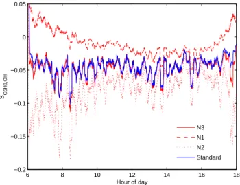
To test the effect of heterogeneous NO concentrations, three further runs were carried out constrained to a randomly-generated normally distributed isoprene time-series. The first of these runs, N1, was constrained to a NO mixing ratio of 50 pptv if isoprene mixing ratios were greater than 2.5 ppbv, 10 pptv if isoprene mixing ratios were less than 1.5 ppbv, and 30 pptv if isoprene mixing ratios were between 1.5 and 2.5 ppbv. This produced an effect where high NO concen-trations were more typically co-located with high isoprene concentrations; an effect that may well occur if coupling of the canopy to the BL is the primary reason for heterogeneous concentration distributions. The second of these runs, N2, was identical except a NO mixing ratio of 10 pptv was used if isoprene mixing ratios were greater than 2.5 ppbv, and a NO mixing ratio of 50 pptv was used if isoprene mixing ra-tios were less than 1.5 ppbv, resulting in a scenario where high NO concentrations were typically anti-correlated with high isoprene concentrations. Finally N3 was constrained to a randomly-generated NO time-series that was entirely inde-pendent of isoprene.
Figure 9 shows the results for runs N1, N2 and N3, com-pared to the standard run for that day. Run N1 shows a substantial decrease in segregation, with much less negative
SC5H8,OH, as found by Krol et al. (2000). Indeed, at the ends
of the day, when OH production via photolysis is relatively small compared to production via the reaction of peroxy rad-icals with NO,SC5H8,OHcan even become positive as the
ef-fect on [OH] caused by increased [NO] dominates over the effect caused by decreased isoprene.
Run N2 has the opposite effect, showing that NO concen-trations anti-located with isoprene concenconcen-trations could yield significantly more negative values of SC5H8,OH. However,
6 8 10 12 14 16 18 −0.2
−0.15 −0.1 −0.05 0 0.05
Hour of day
SC5H8,OH
N3
N1
N2
Standard
Fig. 9. The effect of heterogeneous NO concentrations correlated with those of isoprene (N1, red dashes), anti-correlated with those of isoprene (N2, red dots), and showing no correlation with iso-prene (N3, red line), compared with a standard run (blue line) for a randomly-generated isoprene time-series.
these species is unlikely, since NO emissions from the soil must transit past the isoprene-rich canopy to reach the BL. Aircraft measurements indicate that [NOx] in the free tropo-sphere is much lower than that in the BL (Hewitt et al., 2009), ruling out a free tropospheric NOxsource which could cause an anti-correlation. Therefore, we deduce that the most likely scenario is either N1, or that the distributions of NO and iso-prene in the BL will simply be different and uncorrelated. Run N3 demonstrates that if any heterogeneities in the NO concentration are independent of those in the isoprene con-centration, then the typical value ofSC5H8,OH should not be
affected.
Overall the sensitivity tests indicate that our estimation of
SC5H8,OH is likely to represent an upper limit. An increase
inOLdue to unaccounted-for species would tend to decrease
SC5H8,OH, as would plausible covariances of isoprene with
other trace species which could influenceP. For instance, the covariance of isoprene and water vapour is directly anal-ogous to the covariance of isoprene and NO described above.
5 Conclusions
An approach has been described to model the intensity of segregation of isoprene and OH using high temporal resolu-tion isoprene concentraresolu-tion data. The approach shows good agreement when compared with the only observations of iso-prene and OH segregation available in the literature. When the method is applied to measurements made over the south-east Asian tropical rainforest during the OP3 campaign, an intensity of segregation typically less negative than−0.15 is estimated. This is much less negative than the−0.5
re-quired by global and box models of atmospheric chemistry to reconcile their OH and isoprene concentrations with mea-surements. We emphasise that the results of this study are limited to the segregation of isoprene and OH alone, and not the segregation of any other species with OH.
The model-estimated intensity of segregation for the OP3 rainforest scenario described in this paper is subject to many unconstrained uncertainties; in particular the distribution of OH sources and non-isoprene OH sinks. However, the na-ture of the processes involved is such that these uncertainties would tend the result towards less negative values of inten-sity of segregation. The result appears robust to potential OH recycling, unless such recycling happens virtually instanta-neously following initial isoprene oxidation. Given that rapid isoprene concentration measurements have been made dur-ing several other field campaigns, it is suggested that the ap-proach described here might be applied to estimate the inten-sity of segregation in those regions.
Both Butler et al. (2008) and Pugh et al. (2010) have demonstrated that additional OH recycling in the isoprene oxidation scheme can only improve model fits to measured OH concentrations at the expense of the fit to measured iso-prene concentrations/fluxes. In order to attain an acceptable fit to both OH and isoprene concentrations a reduction in
kC5H8,OH was required. However this work shows that, at
least for the rainforest conditions observed during the OP3 campaigns in Malaysia, segregation of isoprene and OH can only be responsible for a minor fraction of the rate constant reduction required to resolve the measurement-model dis-crepancy; hence either another justification for thiskC5H8,OH
reduction must be made or an alternative solution found. In the light of the results presented here, it is suggested that the highest temporal resolution measurements for isoprene available are utilised in constrained modelling studies of at-mospheric chemistry in areas where isoprene dominates the OH sink. If high temporal resolution measurements of other species are co-located with the isoprene measurement (i.e. sufficiently close that they are very likely measuring within the same air parcel) then it may prove advantageous to use these also.
Appendix A
The timescale for the OH concentration to reach a new steady state following a perturbation in the isoprene mixing ratio from 2 to 3 ppbv (assuming no other OH sinks), is found by integrating the volume average conservation equation:
∂hOHi
∂t =P−kC5H8,OHhOHihC5H8i (A1)
where,
P=kO1D,H 2OhO
1
0 10 20 30 40 50 60 70 80 90 100 0
1 2
C5 H8
(ppbv)
Time (seconds)
0 10 20 30 40 50 60 70 80 90 1000.5
1 1.5 2 2.5
[OH] (
×
10
6 molecules cm
−3
)
Fig. A1. Response of modelled [OH] to a change in the supplied C5H8. Each model time-point is marked by a dot.
to yield
t=
−1
kC5H8,OHhC5H8i
lnP−kC5H8,OHhOHihC5H8i
hOHit
hOHi0
(A3) wherehOHi0is the OH concentration att= 0 andhOHit is
the OH concentration at timet, when the system is in steady state. At steady state∂hOHi/∂t=0, therefore,
P=kC5H8,OHhOHihC5H8i (A4)
Hence the hOHit limit of Eq. A3 is zero. When a
P= 3.0×10⁶moleculescm−3s−1is used,t=3 s. This value of
P is based upon midday typical midday values of the com-ponents of Eq. (A2) during the OP3 campaign (Hewitt et al., 2010). As the approach to steady state is exponential in na-ture, the majority of this change in [OH] due to a perturba-tion in [C5H8] will occur within 1 s. This is demonstrated in Fig. A1 which shows an extract of the model time-series for C5H8(blue) and OH (green). Each mark represents a model timestep of one second. It is clear that the OH response to a change in C5H8concentration occurs nearly entirely within the first timestep following the change.
Acknowledgements. The authors wish to thank A. Jarvis for stimulating the discussion that led to this work and for helpful comments, P. Di Carlo for sharing his NO2data, and P. H. Haynes
(DAMTP, Cambridge) and K. Ashworth for their kind assistance with the analysis. They also wish to acknowledge the advice of two anonymous reviewers, whose comments greatly improved the clarity of the manuscript. We thank the Malaysian and Sabah Governments for their permission to conduct research in Malaysia; the Malaysian Meteorological Department for access to the Bukit Atur Global Atmosphere Watch station; Waidi Sinun of Yayasan Sabah and his staff, Glen Reynolds of the Royal Society’s South East Asian Rainforest Research Programme and his staff, and Nick Chappell and Brian Davison of Lancaster University for logistical support at the Danum Valley Field Centre. The work was funded by
the Natural Environment Research Council Grants NE/D002117/1
and NE/E011179/1. This is paper number 508 of the Royal
Society’s South East Asian Rainforest Research Programme.
Edited by: A. B. Guenther
References
Brown, P., Byrne, G., and Hindmarsh, A.: VODE –A Variable-coefficient ODE solver, Siam J. Sci. Stat. Comp.,, 10, 1038– 1051, 1989.
Butler, T. M., Taraborrelli, D., Br¨uhl, C., Fischer, H., Harder, H., Martinez, M., Williams, J., Lawrence, M. G., and Lelieveld, J.: Improved simulation of isoprene oxidation chemistry with the ECHAM5/MESSy chemistry-climate model: lessons from the GABRIEL airborne field campaign, Atmos. Chem. Phys., 8, 4529–4546, doi:10.5194/acp-8-4529-2008, 2008.
Carslaw, N., Creasey, D., Harrison, D., Heard, D., Hunter, M., Ja-cobs, P., Jenkin, M., Lee, J., Lewis, A., Pilling, M., Saunders, S., and Seakins, P.: OH and HO2radical chemistry in a forested
re-gion of north-western Greece, Atmos. Environ., 35, 4725–4737, 2001.
Dlugi, R., Berger, M., Zelger, M., Hofzumahaus, A., Siese, M., Holland, F., Wisthaler, A., Grabmer, W., Hansel, A., Koppmann, R., Kramm, G., M¨ollmann-Coers, M., and Knaps, A.: Turbulent exchange and segregation of HOxradicals and volatile organic
compounds above a deciduous forest, Atmos. Chem. Phys., 10, 6215–6235, doi:10.5194/acp-10-6215-2010, 2010.
Donovan, R., Hope, E., Owen, S., Mackenzie, A., and Hewitt, C.: Development and Application of an Urban Tree Air Qual-ity Score for Photochemical Pollution Episodes Using the Birm-ingham, United Kingdom, Area as a Case Study, Environ. Sci. Technol., 39, 6730–6738, 2005.
Emmerson, K. M., MacKenzie, A. R., Owen, S. M., Evans, M. J., and Shallcross, D. E.: A Lagrangian model with simple primary and secondary aerosol scheme 1: comparison with UK PM10 data, Atmos. Chem. Phys., 4, 2161–2170, doi:10.5194/acp-4-2161-2004, 2004.
Emmerson, K., Carslaw, N., Carpenter, L., Heard, D., Lee, J., and Pilling, M.: Urban atmospheric chemistry during the PUMA
campaign 1: Comparison of modelled OH and HO2
concen-trations with measurements, J. Atmos. Chem., 52, 143–164, doi:10.1007/s10874-005-1322-3, 2005.
Emmerson, K. M., Carslaw, N., Carslaw, D. C., Lee, J. D., McFig-gans, G., Bloss, W. J., Gravestock, T., Heard, D. E., Hopkins, J., Ingham, T., Pilling, M. J., Smith, S. C., Jacob, M., and Monks, P. S.: Free radical modelling studies during the UK TORCH Campaign in Summer 2003, Atmos. Chem. Phys., 7, 167–181, doi:10.5194/acp-7-167-2007, 2007.
Evans, M., Shallcross, D., Law, K., Wild, J., Simmonds, P., Spain, T., Berrisford, P., Methven, J., Lewis, A., McQuaid, J., Pilling, M., Bandy, B., Penkett, S., and Pyle, J.: Evaluation of a La-grangian box model using field measurements from EASE (East-ern Atlantic Summer Experiment) 1996, Atmos. Environ., 34, 3843–3863, 2000.
Chemistry Project (IGAC), Bologna, Italy, 13–17 September, 1999, 2000.
Guenther, A., Hewitt, C., Erickson, D., Fall, R., Geron, C., Graedel, T., Harley, P., Klinger, L., Lerdau, M., McKay, W., Pierce, T., Scholes, B., Steinbrecher, R., Tallamraju, R., Taylor, J., and Zim-merman, P.: A global model of natural volatile organic com-pound emissions, J. Geophys. Res., 100, 8873–8892, 1995. Hayward, S., Hewitt, C., Sartin, J., and Owen, S.:
Perfor-mance characteristics and applications of a proton transfer reaction-mass spectrometer for measuring volatile organic com-pounds in ambient air, Environ. Sci. Tech., 36, 1554–1560, doi:10.1021/es0102181, 2002.
Helfter, C., Phillips, G., Coyle, M., Di, Marco, C., Langford, B., Whitehead, J., Dorsey, J., Gallagher, M., Sei, E., Fowler, D., and Nemitz, E.: Momentum and heat exchange above South East Asian rainforest in complex terrain, Atmos. Chem. Phys. Dis-cuss., in preparation, 2010.
Hewitt, C. N., MacKenzie, A. R., Di Carlo, P., Di Marco, C. F., Dorsey, J. R., Evans, M., Fowler, D., Gallagher, M. W., Hop-kins, J. R., Jones, C. E., Langford, B., Lee, J. D., Lewis, A. C., Lim, S. F., McQuaid, J., Misztal, P., Moller, S. J., Monks, P. S., Nemitz, E., Oram, D. E., Owen, S. M., Phillips, G. J., Pugh, T. A. M., Pyle, J. A., Reeves, C. E., Ryder, J., Siong, J., Skiba, U., and Stewart, D. J.: Nitrogen management is essential to prevent tropical oil palm plantations from causing ground-level ozone pollution, P. Natl. Acad. Sci. USA, 106, 18447–18451, doi:10.1073/pnas.0907541106, 2009.
Hewitt, C. N., Lee, J. D., MacKenzie, A. R., Barkley, M. P., Carslaw, N., Carver, G. D., Chappell, N. A., Coe, H., Col-lier, C., Commane, R., Davies, F., Davison, B., DiCarlo, P., Di Marco, C. F., Dorsey, J. R., Edwards, P. M., Evans, M. J., Fowler, D., Furneaux, K. L., Gallagher, M., Guenther, A., Heard, D. E., Helfter, C., Hopkins, J., Ingham, T., Irwin, M., Jones, C., Karunaharan, A., Langford, B., Lewis, A. C., Lim, S. F., MacDonald, S. M., Mahajan, A. S., Malpass, S., McFiggans, G., Mills, G., Misztal, P., Moller, S., Monks, P. S., Nemitz, E., Nicolas-Perea, V., Oetjen, H., Oram, D. E., Palmer, P. I., Phillips, G. J., Pike, R., Plane, J. M. C., Pugh, T., Pyle, J. A., Reeves, C. E., Robinson, N. H., Stewart, D., Stone, D., Whalley, L. K., and Yang, X.: Corrigendum to ”Overview: oxidant and particle photochemical processes above a south-east Asian tropical rain-forest (the OP3 project): introduction, rationale, location charac-teristics and tools” published in Atmos. Chem. Phys., 10, 169– 199, 2010, Atmos. Chem. Phys., 10, 563–563, doi:10.5194/acp-10-563-2010, 2010.
Hofzumahaus, A., Rohrer, F., Lu, K., Bohn, B., Brauers, T., Chang, C.-C., Fuchs, H., Holland, F., Kita, K., Kondo, Y., Li, X., Lou, S., Shao, M., Zeng, L., Wahner, A., and Zhang, Y.: Amplified Trace Gas Removal in the Troposphere, Science, 324, 1702– 1704, doi:10.1126/science.116456, 2009.
IUPAC: Evaluated kinetic data, http://www.iupac-kinetic.ch.cam. ac.uk/, last access: 19th March 2009, 2009.
J¨ockel, P., Tost, H., Pozzer, A., Brhl, C., Buchholz, J., Ganzeveld, L., Hoor, P., Kerkweg, A., Lawrence, M. G., Sander, R., Steil, B., Stiller, G., Tanarhte, M., Taraborrelli, D., van Aardenne, J., and Lelieveld, J.: The atmospheric chemistry general circulation model ECHAM5/MESSy1: consistent simulation of ozone from the surface to the mesosphere, Atmos. Chem. Phys., 6, 5067– 5104, doi:10.5194/acp-6-5067-2006, 2006.
Kanaya, Y., Cao, R., Kato, S., Miyakawa, Y., Kajii, Y., Tanimoto, H., Yokouchi, Y., Mochida, M., Kawamura, K., and Akimoto, H.: Chemistry of OH and HO2radicals observed at Rishiri Island, Japan, in September 2003: Missing daytime sink of HO2 and
positive nighttime correlations with monoterpenes, J. Geophys. Res., 112, D11308, doi:10.1029/2006JD007987, 2007.
Kanaya, Y., Pochanart, P., Liu, Y., Li, J., Tanimoto, H., Kato, S., Suthawaree, J., Inomata, S., Taketani, F., Okuzawa, K., Kawa-mura, K., Akimoto, H., and Wang, Z. F.: Rates and regimes of photochemical ozone production over Central East China in June 2006: a box model analysis using comprehensive measure-ments of ozone precursors, Atmos. Chem. Phys., 9, 7711–7723, doi:10.5194/acp-9-7711-2009, 2009.
Kleffmann, J., Gavriloaiei, T., Hofzumahaus, A., Holland, F., Koppmann, R., Rupp, L., Schlosser, E., Siese, M., and Wah-ner, A.: Daytime formation of nitrous acid: A major source of OH radicals in a forest, Geophys. Res. Lett., 32, L05818, doi:10.1029/2005GL022524, 2005.
Krol, M., Molemaker, M., and Vil`a Guerau de Arellano, J.: Effects of turbulence and heterogeneous emissions on photochemically active species in the convective boundary layer, J. Geophys. Res., 105, 6871–6884, 2000.
Kubistin, D., Harder, H., Martinez, M., Rudolf, M., Sander, R., Bozem, H., Eerdekens, G., Fischer, H., Gurk, C., Kl¨upfel, T., K¨onigstedt, R., Parchatka, U., Schiller, C. L., Stickler, A., Taraborrelli, D., Williams, J., and Lelieveld, J.: Hydroxyl rad-icals in the tropical troposphere over the Suriname rainforest: comparison of measurements with the box model MECCA, At-mos. Chem. Phys., 10, 9705–9728, doi:10.5194/acp-10-9705-2010, 2010.
Langford, B., Misztal, P. K., Nemitz, E., Davison, B., Helfter, C., Pugh, T. A. M., MacKenzie, A. R., Lim, S. F., and He-witt, C. N.: Fluxes and concentrations of volatile organic com-pounds from a South-East Asian tropical rainforest, Atmos. Chem. Phys., 10, 8391–8412, doi:10.5194/acp-10-8391-2010, doi:10.5194/acp-10-8391-2010, 2010.
Lawrence, M., Crutzen, P., Rasch, P., Eaton, B., and Mahowald, N.: A model for studies of tropospheric photochemistry: Descrip-tion, global distributions, and evaluaDescrip-tion, J. Geophys. Res., 104, 26245–26277, 1999.
Lelieveld, J., Peters, W., Dentener, F., and Krol, M.: Stabil-ity of tropospheric hydroxyl chemistry, J. Geophys. Res., 107, doi:10.1029/2002JD002272, 2002.
Lelieveld, J., Butler, T. M., Crowley, J. N., Dillon, T. J., Fis-cher, H., Ganzeveld, L., Harder, H., Lawrence, M. G., Martinez, M., Taraborrelli, D., and Williams, J.: Atmospheric oxidation capacity sustained by a tropical forest, Nature, 452, 737–740, doi:10.1038/nature06870, 2008.
Martinez, M., Harder, H., Kubistin, D., Rudolf, M., Bozem, H., Eerdekens, G., Fischer, H., Klpfel, T., Gurk, C., Knigstedt, R., Parchatka, U., Schiller, C. L., Stickler, A., Williams, J., and Lelieveld, J.: Hydroxyl radicals in the tropical troposphere over the Suriname rainforest: airborne measurements, Atmos. Chem. Phys., 10, 3759–3773, doi:10.5194/acp-10-3759-2010, 2010. McMillen, R.: An eddy-correlation technique with extended
appli-cability to non-simple terrain, Bound.-Lay. Meteorol., 43, 231– 245, 1988.
Me-teorol., 100, 91–129, 2001.
Pearson, G., Davies, F., and Collier, C.: Remote sensing of the tropical rain forest boundary layer using pulsed Doppler lidar, Atmos. Chem. Phys., 10, 5891–5901, doi:10.5194/acp-10-5891-2010, 2010.
Peeters, J., Nguyen, T. L., and Vereecken, L.: HOxradical
regener-ation in the oxidregener-ation of isoprene, Phys. Chem. Chem. Phys., 11, 5935–5939, doi:10.1039/b908511d, 2009.
Poisson, N., Kanakidou, M., and Crutzen, P.: Impact of non-methane hydrocarbons on tropospheric chemistry and the oxidiz-ing power of the global troposphere: 3-dimensional modelloxidiz-ing results, J. Atmos. Chem., 36, 157–230, 2000.
Powell, D. and Elderkin, C.: Investigation of application of Taylor’s hypothesis to atmospheric boundary-layer turbulence, J. Atmos. Sci., 31, 990–1002, 1974.
Pugh, T. A. M., MacKenzie, A. R., Hewitt, C. N., Langford, B., Edwards, P. M., Furneaux, K. L., Heard, D. E., Hopkins, J. R., Jones, C. E., Karunaharan, A., Lee, J., Mills, G., Misztal, P., Moller, S., Monks, P. S., and Whalley, L. K.: Simulating atmo-spheric composition over a South-East Asian tropical rainforest: performance of a chemistry box model, Atmos. Chem. Phys., 10, 279–298, doi:10.5194/acp-10-279-2010, 2010.
Real, E., Law, K. S., Weinzierl, B., Fiebig, M., Petzold, A., Wild, O., Methven, J., Arnold, S., Stohl, A., Huntrieser, H., Roiger, A., Schlager, H., Stewart, D., Avery, M., Sachse, G., Browell, E., Ferrare, R., and Blake, D.: Processes influenc-ing ozone levels in Alaskan forest fire plumes durinfluenc-ing long-range transport over the North Atlantic, J. Geophys. Res., 112, doi:10.1029/2006JD007576, 2007.
Real, E., Law, K. S., Schlager, H., Roiger, A., Huntrieser, H., Methven, J., Cain, M., Holloway, J., Neuman, J. A., Ryerson, T., Flocke, F., de Gouw, J., Atlas, E., Donnelly, S., and Parrish, D.: Lagrangian analysis of low altitude anthropogenic plume pro-cessing across the North Atlantic, Atmos. Chem. Phys., 8, 7737– 7754, doi:10.5194/acp-8-7737-2008, 2008.
Ren, X., Olson, J. R., Crawford, J. H., Brune, W. H., Mao, J., Long, R. B., Chen, Z., Chen, G., Avery, M. A., Sachse, G. W., Bar-rick, J. D., Diskin, G. S., Huey, L. G., Fried, A., Cohen, R. C., Heikes, B., Wennberg, P. O., Singh, H. B., Blake, D. R., and Shetter, R. E.: HOxchemistry during INTEX-A 2004:
Observa-tion, model calculaObserva-tion, and comparison with previous studies, J. Geophys. Res., 113, D05310, doi:10.1029/2007JD009166, 2008. Schumann, U.: Large-eddy simulation of turbulent-diffusion with chemical-reactions in the convective boundary-layer , Atmos. Environ., 23, 1713–1727, 1989.
Spirig, C., Neftel, A., Ammann, C., Dommen, J., Grabmer, W., Thielmann, A., Schaub, A., Beauchamp, J., Wisthaler, A., and Hansel, A.: Eddy covariance flux measurements of biogenic VOCs during ECHO 2003 using proton transfer re-action mass spectrometry, Atmos. Chem. Phys., 5, 465–481, doi:10.5194/acp-5-465-2005, 2005.
Sykes, R., Parker, S., Henn, D., and Lewellen, W.: Turbulent mixing with chemical-reaction in the planetary boundary-layer , J. Appl. Meteorol., 33, 825–834, 1994.
Tan, D., Faloona, I., Simpas, J., Brune, W., Olson, J., Crawford, J., Avery, M., Sachse, G., Vay, S., Sandholm, S., Guan, H., Vaughn, T., Mastromarino, J., Heikes, B., Snow, J., Podolske, J., and Singh, H.: OH and HO2in the tropical Pacific: Results from
PEM-Tropics B, J. Geophys. Res., 106, 32667–32681, 2001. Vil`a Guerau de Arellano, J., Duynkerke, P., and Zeller, K.:
Atmo-spheric surface-layer similarity theory applied to chemically re-active species, J. Geophys. Res. Atm., 100, 1397–1408, 1995. Vinuesa, J. and Vil`a Guerau de Arellano, J.: Fluxes and
(co-)variances of reacting scalars in the convective boundary layer, Tellus B, 55, 935–949, 2003.
Vinuesa, J. and Vil`a Guerau de Arellano, J.: Introducing effec-tive reaction rates to account for the inefficient mixing of the convective boundary layer, Atmos. Environ., 39, 445–461, doi:10.1016/j.atmosenv.2004.10.003, 2005.
Vinuesa, J.-F. and Porte-Agel, F.: Dynamic models for the subgrid-scale mixing of reactants in atmospheric turbulent reacting flows, J. Atmos. Sci., 65, 1692–1699, doi:10.1175/2007JAS2392.1, 2008.
von Kuhlmann, R., Lawrence, M., Poschl, U., and Crutzen, P.: Sen-sitivities in global scale modeling of isoprene, Atmos. Chem. Phys., 4, 1–17, 2004.
Wang, Y., Jacob, D., and Logan, J.: Global simulation of tro-pospheric O3-NOx-hydrocarbon chemistry 3. Origin of
tropo-spheric ozone and effects of nonmethane hydrocarbons, J. Geo-phys. Res., 103, 10757–10767, 1998.
Whalley, L. K., Edwards, P. M., Furneaux, K. L., Goddard, A., Ingham, T., Evans, M. J., Stone, D., Hopkins, J. R., Jones, C. E., Karunaharan, A., Lee, J. D., Lewis, A. C., Monks, P. S., Moller, S. J., and Heard, D. E.: Quantifying the magnitude of a missing hydroxyl radical source in a tropical rainforest, At-mos. Chem. Phys. Discuss., 11, 5785–5809, doi:10.5194/acpd-11-5785-2011, 2011.
Wild, O., Law, K., McKenna, D., Bandy, B., Penkett, S., and Pyle, J.: Photochemical trajectory modeling studies of the North At-lantic region during August 1993, J. Geophys. Res., 101, 29 269– 29 288, 1996.


![Fig. A1. Response of modelled [OH] to a change in the supplied C 5 H 8 . Each model time-point is marked by a dot.](https://thumb-eu.123doks.com/thumbv2/123dok_br/17166732.241026/12.892.77.425.96.354/fig-response-modelled-change-supplied-model-point-marked.webp)
