Suppression of Anderson localization of light in one-dimensional disordered photonic superlattices
E. Reyes-G´omez,1A. Bruno-Alfonso,2S. B. Cavalcanti,3and L. E. Oliveira4 1Instituto de F´ısica, Universidad de Antioquia, AA 1226, Medell´ın, Colombia 2Faculdade de Ciˆencias, UNESP-Universidade Estadual Paulista, 17033-360, Bauru-SP, Brazil
3Instituto de F´ısica, Universidade Federal de Alagoas, Macei´o-AL, 57072-970, Brazil 4Instituto de F´ısica, Universidade Estadual de Campinas-UNICAMP, Campinas-SP, 13083-859, Brazil
(Received 2 February 2012; published 7 May 2012)
The localization properties of electromagnetic modes in one-dimensional disordered photonic superlattices are theoretically studied. The multilayered system is considered to be composed of alternating stacks of two different random-thickness slabs, characterized by nondispersive and/or frequency-dependent electric permittivities and magnetic permeabilities. Results for the localization length are evaluated by using an analytical model for weakly disordered systems as well as its general definition through the transmissivity properties of the heterostructure. Good agreement between both results is observed only for small amplitudes of disorder. The critical frequencies at which the localization length diverges are correctly predicted in the whole frequency spectrum by the analytical model and confirmed via the corresponding numerical calculations. Theλ2dependence of the localization length, previously observed in disordered heterostructures made of material of positive refractive indexes, are confirmed in the present work. In addition, newλ4andλ−4 dependencies of the localization length in positive-negative disordered photonic superlattices are obtained, under certain specific conditions, in the long and short wavelength limits, respectively. The asymptotic behavior of the localization length in these limits is essentially determined by the particular frequency dispersion that characterizes the metamaterial used in the left-handed layers. When the effects of absorption are considered, then a divergence of the localization length is still observed, under some conditions, in the short wavelength limit.
DOI:10.1103/PhysRevB.85.195110 PACS number(s): 78.67.Pt, 42.25.Dd, 72.15.Rn
I. INTRODUCTION
The complex and fascinating physics behind Anderson localization1 has stimulated a rich variety of theoretical and experimental work, worldwide, on the nature of wave propagation in random media. Characterized originally by the vanishing of the electronic diffusion in disordered media, this interference wave phenomenon has been investigated in all sorts of waves, from electromagnetic to seismic ones. Anderson localization has been observed in classical wave sys-tems such as microwave, light, and ultrasound.2The vectorial character of the electromagnetic waves may provide interesting phenomena not known in their electronic counterpart. The microstructuring techniques of high-quality optical materials, available nowadays, have given a new thrust to develop further studies on this important and puzzling phenomenon. Disorder and localization effects on light propagation in photonic crystals (PC) have been investigated both theoretically and experimentally.3,4 Due to the remarkable flexibility in the fabrication of new materials, one is able to tailor the electro-magnetic dispersion relation and mode structure of a material to suit almost any need,5 such as the simultaneous negative electric permittivity and magnetic permeability of a so-called metamaterial or a left-handed material (LHM) in contrast with the usual right-handed material (RHM), an allusion to the vectorial product between the electric and magnetic fields.6 To ensure positiveness of the electromagnetic energy density,7 a LHM must be dispersive. Furthermore, it exhibits optical magnetism.8,9This particular feature induces new possibilities for the control of light propagation, such as negative refraction, superlens, and cloaking.10–12 A study on a one-dimensional (1D) structure composed of alternate layers of air and a nondispersive LHM, where the disorder was introduced by
randomizing the refractive indices of the layers, has indicated strong suppression of Anderson localization13,14 and unusual behavior of the localization lengthξat long wavelengthsλ, in contrast with the well-knownξ ∝λ2 asymptotic behavior.15 Although in Refs. 13 and 14 it was shown that ξ ∝λ6,
this result is essentially due to the insufficient size of the systems considered in the numerical calculations, and a recent analytical study16 indicated that, in such systems, the correct asymptotic behavior of the localization length isξ ∝λ8.
have illustrated the influence of the combination dispersion-quasiperiodicity on the localization length.19The effects of the absorption on the Anderson localization of electromagnetic waves in weakly disordered systems were also theoretically investigated.20 Such studies reveal that delocalized modes, obtained from numerical simulations in nonabsorptive media, are gradually suppressed as the absorption level is increased.
In the present work, we set out to investigate the influence of the particular medium response on the localization length of 1D stacks composed of nondispersive RHM-RHM or RHM-LHM superlattices, in which the LHM layer is con-sidered dispersive, in order to understand the behavior of the localization length under various types of medium responses. This paper is organized as follows: In Sec.IIthe theoretical procedure is described. In Sec.IIIwe show the results obtained for various types of heterostructures: a nondispersive RHM-RHM superlattice, a RHM-RHM-LHM superlattice in which the LHM is characterized by Drude-type responses, and, finally, a RHM-LHM superlattice with the LHM characterized by a dispersive split-ring resonator (SRR) electric permittivity and magnetic permeability, with and without absorption effects. SectionIVpresents our conclusions that amounts to say that the asymptotic behavior of the localization length depends crucially on the particular medium response.
II. THEORETICAL FRAMEWORK
Here we consider a multilayered system composed of alternating stacks of two different slabs of optical materials A andB, which are characterized by electric permittivities and magnetic permeabilities ǫA and μA, and ǫB and μB,
respectively. The multilayered system under consideration is supposed to be sandwiched between two semi-infinite layers of material A. The widthaj (bj) of the layerA (B) at the
jth site of the multilayered system is defined asaj =a+δAj
(bj =b+δjB), whereδjA(δBj) are random variables uniformly
distributed in the interval [−A/2,A/2] ([−B/2,B/2]).
ParametersAandB are then the amplitudes of disorder of
layersA andB, respectively. Further, we assume that there is no correlation between the disorder of the heterostructure slabs.22 In what follows, the symbol
... represents the configurational average of a given geometrical or physical variable, i.e., the average taken over a sufficiently large ensemble of multilayered systems, in which each element of the ensemble corresponds to a system obtained for a single realization of disorder. One may note that a= aj
andb= bj.
In order to calculate the localization length of the electro-magnetic modes in the multilayered heterostructure, it is, first, necessary to calculate the light-transmission coefficientT of the photonic heterostructure. The transfer-matrix formalism may be used for such purposes.17–19 Once the transmission coefficient is obtained for each member of the ensemble, the localization length ξ may be evaluated through the expression15,23
ξ−1 = − lim
N→∞
ln(T) 2L
, (1)
whereNis the number of double layers (AB) in the photonic system andL=N
j=1(aj +bj) is the length of the photonic
heterostructure. For practical purposes, the limitN → ∞in Eq. (1) is reached for a sufficiently large number of layers in each photonic heterostructure of the ensemble over which the configurational average is taken.19 It is also necessary to explain how the number of elements of such ensemble, i.e., the number of disorder realizations, is chosen. The single-parameter scaling (SPS) principle dictates that var(l)=l, where var(l)= l2
− l2is the variance of the dimensionless
Lyapunov exponentl= L/ξ, andLis the average system length.24,25The SPS principle indicates that large values ofl lead to large values of the variance var(l) and, therefore, to large fluctuations of the Lyapunov exponent around its mean value. It then would be important to set up an appropriate value of the number of realizations to take the configurational average. Nevertheless, the SPS principle is violated under some specific conditions and, therefore, it cannot be straightforwardly used to predict the behavior of var(l) from the value of the Lyapunov exponent.24,25 Consequently, an estimation of the optimal number of realizations sufficient to achieve the convergence of Eq.(1)cannot be trivially obtained, by using the SPS principle, from ana priorivalue of the localization length. The number of realizations used in the present paper was chosen by studying the convergence of the localization length, as a function of the number of realizations, for a collection of some frequency values. We noted that, in most of cases discussed below, numerical results for the localization length stabilized around 50–90 realizations of disorder (the study of the convergence will not be shown here).
Although Eq. (1) provides a general way to obtain the localization length in 1D disordered heterostructures, for weakly disordered systems it is possible to derive an analytical expression forξ in terms of parameters corresponding to a 1D finite photonic crystal without disorder, with slabsAandB of widthsaandb, respectively. It has been shown17,22that, in this case, the localization length may be obtained as
ξ−1= K
8dsin2(kd), (2)
whered =a+b,kis the 1D Bloch wave vector in the perfect photonic crystal and
K=F−2Q2AσA2sin2(QBb)+Q2Bσ 2 Bsin
2
(QAa)
. (3)
The variances σ2 A= (δ
A j)
2 =2
A/12 and σ 2 B = (δ
B j)
2 = 2B/12 account for the degrees of disorder of the slabs A andB, respectively, whereas sin2(kd) may be computed from the transcendental equation giving the dispersion relation of the periodic 1D photonic crystal, i.e.,
cos(kd)=cos(QAa) cos(QBb)−12F+sin(QAa) sin(QBb).
(4)
In the above expressions one has
F±= fA fB ±
fB
fA
where the functions fx (x = A, B), for the TE and TM
polarizations, are given by
fxTE= ux μx
and fxTM= ux ǫx
, (6)
respectively, ux =
ǫxμx−sin2θ,Qx=(ω/c)ux, and θ is
the incidence angle relative to the vacuum. Equation (2) was recently derived by Izrailev and Makarov22 and was generalized by Mogilevtsevet al.17 to include the possibility of oblique incidence. Hereafter we refer to this equation as the Izrailev-Makarov (I-M) equation,22which was perturbatively obtained under the assumptions that, in the multilayered system, the field phase is homogeneously distributed and the disorder is weak. In other words, the disorder amplitudes should be much less than the mean widths of the slabs composing the heterostructure, and the conditionsQ2
xσx2≪1
(withx=A, B) should be satisfied22in order to use Eq.(2). This fact is of particular importance in dispersive superlattices, where the productQ2
xσx2may be divergent in the limitω→0,
ω→ ∞or even at a finite value of the frequency. Therefore, the particular frequency dependencies of bothǫ(ω) andμ(ω) in each material of the heterostructure will determine the frequency regions where Eq.(2)is applicable.
We now consider the I-M equation in some detail and refer to the localization length as obtained from Eq.(2). We are interested in studying the frequency values at which the localization length diverges, yielding extended states in the disordered multilayered system. We denote such frequency values asωccritical frequencies. Of course,ωcshould be real
and non-negative. By taking into account Eq. (4), one may note that the inequality
|cos(QAa) cos(QBb)−12F+sin(QAa) sin(QBb)|1 (7)
should be satisfied in the limitω→ωc.
We, first, analyze the case of normal incidence (θ=0), a situation in which one may expect that the condition
lim
ω→ωc
K(ω)=0 (8)
should be accomplished. In this case (θ=0), the functionK may be written as
K(ω)=ω
2
c2 gN(ω)hN(ω), (9)
where
gN(ω)=[ǫA(ω)μB(ω)−ǫB(ω)μA(ω)]2 (10)
and
hN(ω)=σA2
sin2ωb c
√
ǫB(ω)μB(ω)
ǫB(ω)μB(ω)
+σB2sin
2ωa c
√
ǫA(ω)μA(ω)
ǫA(ω)μA(ω)
. (11)
If the critical frequencies come from the zeros ofgN, then one
may see thatZ2A(ωc)=ZB2(ωc), where
Zx(ω)= √
μx(ω) √
ǫx(ω)
(12)
is the optical impedance of mediumx=Aorx =B. In other words, the suppression of the Anderson localization would be
due, in this case, to the matching of the square of the optical impedance throughout the multilayered system. As it is known, the impedance matching of two different media leads to the vanishing of the reflectivity at the interface between them,22,26 a fact which results in an enhancement of the transmissivity and, as a consequence, in an increase of the localization length. The critical frequencies obtained from the conditiongN(ω)=
0 do not depend on the geometrical parameters or degree of disorder of the multilayered system and are determined by the frequency dependence of the electric permittivities and magnetic permeabilities of slabsAandB.
In the absence of absorption effects, i.e., for electricǫxand
magneticμx responses assumed as real functions, a careful
analysis of Eq. (11) indicates that the zeros of hN are not
critical frequencies. In fact, the equationhN(ω)=0 has no real
solutions unless the conditions ωa c
√
ǫA(ω)μA(ω)=m1π and ωb
c √
ǫB(ω)μB(ω)=m2πare simultaneously met for a certain
value of the frequency, wherem1andm2are nonzero integer
numbers. According to Eq.(4), the above conditions lead to cos(kd)= ±1 and, therefore, to the vanishing of sin2(kd) in
the denominator of Eq.(2). Nevertheless, it is possible to show that the localization length remains finite as the frequency approaches the zeros ofhN.
As the I-M equation was obtained under the condition Q2
xσx2≪1, withx=AandB, one may expect that it would
not be valid in a frequency region where the above condition does not hold. However, the I-M equation may still be useful to predict the critical frequencies whenQ2xσx21. The reason is the equivalence between the conditions gN(ωc)=0 and
ZA2(ωc)=ZB2(ωc) satisfied by the critical frequency in the case
of normal incidence: The former one is derived from the I-M equation, whereas the second one is general and independent on the degree of disorder.7,22In this way, apart from the positive real zeros ofgN and the caseω=0 [cf. Eq.(9)], one has that
ω→ ∞is a possible candidate to take into account. Ifωc=0
is a critical frequency, then one may expect a suppression of the Anderson localization in the limitλ→ ∞, whereλ=2π c/ω is the vacuum wavelength associated with the electromagnetic wave. Ifωc→ ∞is a critical frequency, then one may expect a
suppression of the Anderson localization in the limitλ→0. Of course, these frequency values are actual critical frequencies only if condition(7)is satisfied.
A similar reasoning applies for oblique incidence. In this case, the delocalization process is often explained in terms of Brewster anomalies17–19: If the incidence angle coincides with the Brewster angle θB, the reflected electromagnetic
wave is suppressed when the incoming monochromatic wave is incident with TM or TE polarization, a fact which gives rise to maximum transmission. In this case the localization length may become larger than the system length and the electromagnetic modes are then delocalized. It is important to stress that, for a given Brewster angle, a set of different frequencies may satisfy the Brewster condition. An important keystone to identify when a critical frequency corresponds to a Brewster anomaly17,18is its strong dependence onθB.
For oblique incidence, one may note thatK in Eq.(2)is given by
K(ω,θ)= ω 2
where
hO(ω,θ)=σA2
sin2ωb c
ǫB(ω)μB(ω)−sin2θ
ǫB(ω)μB(ω)−sin2θ
+σB2 sin2ωa
c
ǫA(ω)μA(ω)−sin2θ
ǫA(ω)μA(ω)−sin2θ
(14)
andgO is defined for TE and TM modes as
gOTE(ω,θ)=
[ǫA(ω)μA(ω)−sin2θ]
μB(ω)
μA(ω)
− [ǫB(ω)μB(ω)−sin2θ]
μA(ω)
μB(ω) 2
(15)
and
gTMO (ω,θ)=
[ǫA(ω)μA(ω)−sin2θ]
ǫB(ω)
ǫA(ω)
− [ǫB(ω)μB(ω)−sin2θ]
ǫA(ω)
ǫB(ω) 2
, (16)
respectively. For a given value of the Brewster angleθB, the
critical frequencies should satisfy
lim
ω→ωc
K(ω,θB)=0. (17)
As in the case of normal incidence, for oblique incidence it is possible to see that, for a given value of the incidence angle θ, the frequency values corresponding to the zeros ofhO(ω,θ)
are not critical frequencies in the absence of absorption. In this case, the possible candidates to critical frequencies areω=0, ω→ ∞, and the positive real values ofωsatisfying equation gXO(ω,θ)=0, withX=TE orX=TM.
Frequenciesω=0 andω→ ∞may be critical frequencies provided that condition(7)is satisfied, thatξ diverges in the limitsω→0 andω→ ∞, respectively, and under conditions that we shall discuss below. In any case,ω=0 andω→ ∞ should not be considered as related with Brewster anomalies. In order to expand on this, we suppose that functionsǫA,μA,
ǫB, andμB have positive finite limitsǫA∞,μ∞A,ǫB∞, andμ∞B,
respectively, asω→ ∞. Moreover, we take (Z∞
A)2=(ZB∞)2,
whereZ∞
A andZB∞are the optical impedances of the slabsA
andB, respectively, in the high-frequency limit. In this case we expect a suppression of the Anderson localization for normal incidence asω→ ∞due to the matching of the square of the optical impedances of the system at this limit. In addition, if condition μ∞
A =μ∞B is satisfied, then the function g TE O
becomes independent ofθ. This fact, combined with condition (ZA∞)
2
=(Z∞B) 2
, leads to the vanishing ofgTEO asω→ ∞and, therefore, to the suppression of the Anderson localization for TE modes in the high-frequency region. A similar situation takes place for TM waves. If ǫ∞
A =ǫB∞, then g TM
O becomes
independent ofθ and tends toward zero asω→ ∞, leading to the suppression of the Anderson localization at this limit. These are cases in which the delocalization process should not be explained in terms of a Brewster anomaly, but one may classify this singularity ofξ as omnidirectional. Furthermore, if μ∞
A =μ∞B (ǫA∞ =ǫB∞) then the localization of TE (TM)
waves occurs for oblique incidence in the high-frequency limit. This analysis may also be extended to the low-frequency region provided that the functionsǫA,μA,ǫB, andμB have
finite limits ǫ0A, μ0A, ǫB0, and μ0B, respectively, as ω→0. Moreover, there may be a physical case in which functions, μA, ǫA, μB, and ǫB have positive or negative finite limits
μjA, ǫAj, μjB, and ǫBj, respectively, at some finite value ωj
of the wave frequency, and that such value of the frequency satisfies inequality(7). If conditionZ2A(ωj)=Z2B(ωj) is valid,
thenωj may be a critical frequency for normal incidence. If
we also haveμA(ωj)= ±μB(ωj) [ǫA(ωj)= ±ǫB(ωj)], then
the function gTE
O (ωj,θ)=0 [gOTM(ωj,θ)=0] regardless of
the value ofθ. Consequently, the TE modes (TM) may be delocalized in such a case and delocalization should not be interpreted as a Brewster anomaly as, although ωj is finite,
it is independent ofθ. As in the limits ω→0 andω→ ∞ analyzed above, delocalization would be omnidirectional at this frequency value. If the remaining positive real zeros ofω satisfying equationgXO(ω,θ)=0 (X=TE orX=TM) also satisfy condition(7), then they may be identified as the usual Brewster anomalies obtained for a given value of the incidence angle.
III. RESULTS AND DISCUSSION A. RHM-RHM nondispersive systems
We, first, consider slabs A and B composed of two different nondispersive materials, for which both magnetic permeabilities and electric permittivities are positive and independent of the wave frequency. For normal incidence one may see that, ifZA2 =ZB2, then the localization length diverges for all values of the wave frequency, as expected.22One may note that if conditionZ2
A =Z2B is satisfied, there is only one
value of the critical frequency,ωc=0. Furthermore, according
to Eq.(4)and Eqs.(9)–(11), it is possible to show that
ξ λ−→→∞ 2 π2
ǫ μ [ǫAμB−ǫBμA]2
d5
σA2b2+σ2 Ba2
λ
d
2
, (18)
whereǫ=(ǫAa+ǫBb)/dandμ=(μAa+μBb)/d. We note
that theλ2 asymptotic behavior of the localization length as λ→ ∞ is a well-known result already reported for RHM-RHM nondispersive multilayered systems.22
To compare the analytical predictions for the localization length obtained from the I-M equation with the numerical results calculated from Eq.(1), we display in Fig.1, for normal incidence, the localization length, as a function of the vacuum wavelength, in a RHM-RHM multilayered system ofN=106
double layers, with the localization length expressed in units of the average system lengthL =N d. For simplicity, we have used the same disorder amplitude for both slabsAand B, i.e.,A=B=. Calculations were performed fora =
b=12μm, and we have chosen the electric permittivities and magnetic permeabilities as in an air-silicon stack (ǫA=μA=
μB =1 andǫB=13.1827). Solid lines in Figs.1(a)and1(b)
10-2 10-1 100 101 102 103 10-8
10-6 10-4 10-2 100 102
ξ
/L
ξ
/L
(b) ΔΔ
= 12
μμm
ξ
/
L
λ λ
/ d
(a) ΔΔ= 1
μμm
~
λλ21 10
10-8 10-6 10-4 10-2
λ λ / d
10-2 10-1 100 101 102 103 10-8
10-6 10-4 10-2 100 102
~
λλ2ξ
/
L
λ λ
/ d
1 10
10-8 10-6 10-4 10-2
λ λ / d
L
L
FIG. 1. (Color online) Localization length for normal incidence, in units of the average system lengthL, as a function of the vacuum wavelength (expressed in units ofd=a+b) in a RHM-RHM multi-layered system ofN=106double layers, witha
=b=12μm,ǫA=
μA=μB=1, andǫB=13.18. Circles and squares correspond to nu-merical results obtained from Eq.(1)for=1μm and=12μm, respectively, and for 100 realizations of disorder. In panels (a) and (b), solid curves correspond to calculations obtained from Eq.(2)for
=1μm and=12μm, respectively, and oblique dashed-dotted lines depict theλ2asymptotic behavior from Eq.(18), for
=1μm and=12μm, respectively. The horizontal dashed lines separate localized and delocalized states. Results are also depicted in the insets for a narrow window of vacuum wavelengths.
length obtained from Eq. (1) remains constant in the limit λ→0. A similar result was reported by Asatryanet al..13,14 Discrepancies are essentially due to the inapplicability of the I-M equation at the short wavelength (or high-frequency) limit in
10-2 10-1 100 101 102 103 10-8
10-6 10-4 10-2 100 102
ξ
/
L
λ λ / d (a) TE
θ = π / 12 Δ = 1 μm
10-2 10-1 100 101 102 103 10-8
10-6 10-4 10-2 100 102
(b) TE
θ = π / 12 Δ = 12 μm
ξ
/
L
λ λ / d
10-2 10-1 100 101 102 103 10-8
10-6 10-4 10-2 100 102
ξ
/
L
λ λ / d (c) TM
θ = π / 12 Δ = 1 μm
10-2 10-1 100 101 102 103 10-8
10-6 10-4 10-2 100 102
(d) TM
θ = π / 12 Δ = 12 μm
ξ
/
L
λ λ / d
FIG. 2. (Color online) As in Fig.1, for oblique incidence (with incidence angleθ=π/12). Results were obtained for the TE [panels (a) and (b)] and TM [panels (c) and (d)] modes.
nondispersive superlattices. In this limit the conditionQ2 xσ
2
x ≪
1 (x =A, B), under which the I-M equation was obtained, is not fulfilled. In the long wavelength limit the I-M equation leads toξ ∝λ2. Numerical calculations obtained from Eq.(1)
also display such behavior ofξ in that limit. AsQ2 xσx2→0
(x=A, B) as λ→ ∞, one may expect a good agreement between the theoretical model and numerical calculations in such a wavelength region. However, for the larger values of λ and for low disorder amplitudes [cf. Fig. 1(a)] one may observe a slight dispersion of the numerical results around the λ2curve. This behavior is essentially due to the finiteness of the
system length, which artificially affects the numerical results obtained from Eq.(1)mainly in the case of≪d, where the localization length is greater than that obtained for∼d. One may note from Fig.1(b)that, for larger disorder amplitude, the λ2 prediction derived from the I-M equation is in good
agreement with numerical results computed from Eq.(1). On the other hand, for intermediate wavelengths, the I-M results and numerical calculations agree only for the smallest value of the disorder amplitude (cf. the insets of Fig.1). A similar situation takes place for oblique incidence, as one may clearly see from Fig.2, where the localization lengths corresponding to TE and TM polarizations are depicted as functions ofλ.
It is apparent from Figs.1and2that the I-M equation de-scribes very well the frequency dependence of the localization length for intermediate wavelengths and in the limitλ→ ∞. In the limitλ→0, however, the localization length remains independent of the wavelength (or frequency), and the I-M model is not applicable.
TABLE I. Conditions for which ωc [cf. Eq. (21)] is a critical frequency, obtained for photonic systems composed by layersAof a nondispersive RHM and LHM layersBwith dispersives electric permittivity and magnetic permeability given by a Drude-like model. Case 1 ωm < ωeZA/Z∞ and Z∞ < ZA Case 2 ωm > ωeZA/Z∞ and Z∞ > ZA Case 3 ωm = ωeZA/Z∞ and Z∞ = ZA Case 4 ωm = ωeZA/Z∞ and Z∞ = ZA
consist of dispersive LHMs with both electric permittivity and magnetic permeability given by the Drude model,28,29i.e.,
ǫB(ω)=ǫ∞
1−ω 2 e
ω2
(19)
and
μB(ω)=μ∞
1−ω
2 m
ω2
, (20)
where ωe and ωm are the electric and magnetic plasmon
frequencies, respectively, and ǫ∞ and μ∞ are the positive electric permittivity and magnetic permeability, respectively, of materialBin the limitω→ ∞.
Let us, first, consider the case of normal incidence. By definingZ∞=√μ∞/√ǫ∞ as the optical impedance of the layersBat infinite frequency, it may be shown that the critical frequency is given by
ωc=
ω2
m−ω2eZA2/Z∞2
1−Z2A/Z2
∞
(21)
under any of the conditions summarized in Table I. Each of such conditions guarantees a real value of ωc and an
optical impedanceZ(ωc) independent on the growth-direction
coordinate. One may note that, if ωm=ωeZA/Z∞ and,
simultaneously, ZA=Z∞, the function gN [cf. Eq. (10)]
vanishes and ξ goes to infinity for all values of the wave frequencyω.
The first two cases shown in Table I lead to finite and nonzero values of the critical frequency, whereas the third and fourth cases lead to critical frequencies equal to zero and infinity, respectively. As a consequence of the Drude-like electric and magnetic responses given by Eqs.(19)and(20), respectively, one may note thatQ2
BσB2 diverges asω→0 (or
λ→ ∞) and ω→ ∞ (or λ→0), whereas Q2 Aσ
2
A diverges
in the limitω→ ∞(λ→0). It must be emphasized that, at these two limits, the I-M equation could not be applied to describe the frequency dependence of the localization length. Nevertheless, it is interesting to obtain the asymptotic behavior of the localization length as a function of the frequency (or vacuum wavelength) by taking the corresponding limits λ→ ∞orλ→0 in Eq.(2). In this sense, if the third condition of TableIis satisfied, one may show, for Drude-like responses, that
ξ λ−→→∞ sin2
2π λ |n(λ)|d
ξmax(λ), (22)
where
ξmax(λ)=∞
λ
d
4
, (23)
∞= d
5
2π4ǫ2 Aμ2∞
1− Z2A Z2
∞
2
σB2a2
, (24)
|n(λ)| = nAa+ |nB(λ)|b
d , (25)
and |nB(λ)| = |√ǫB(2π c/λ)| |√μB(2π c/λ)|. It is apparent
from Eq.(22)that the I-M equation predicts a rapid oscillatory behavior of the localization length in the limit λ→ ∞, provided that the third condition of Table Iis fulfilled. The oscillatory part of the localization length is modulated by λ4, which governs the behavior of the maxima of ξ as functions of λ [cf. Eq. (23)]. The λ4 dependence of the localization length in the long wavelength limit, which is a consequence of the Drude-like frequency dependence of both the electric permittivity and magnetic permeability of layersB [cf. Eqs.(19)and(20)], differs from the asymptotic behavior ofξ previously reported by Asatryan and coworkers13,14 and by Torres-Herreraet al.16
in photonic heterostructures made of layers with random refractive indices. We should also mention that the behaviorξ ∝λ4was obtained for RHM-RHM
1D disordered photonic crystals,22 in the limit λ
→ ∞, by introducing a linear correlation between the fluctuations of the layer widths. Such a physical situation differs from the one studied in the present work, where no correlation between the disorder of the photonic slabs was taken into account.
If the fourth condition of TableIis satisfied, then one may obtain, for Drude-like responses, that
ξ −→λ→0 Ŵ0G0(λ) λ
d
−2
, (26)
where
Ŵ0=
32π2c4
ǫ2 Aμ2∞d
ω2 e−ω2m
2, (27)
G0(λ)=
sin22λπn∞d
σA2sin2[ 2π
λb
√ǫ
∞μ∞]
ǫ∞μ∞ +σ
2 B
sin2[2π λa
√ǫ
AμA] ǫAμA
, (28)
and
n∞= √ǫ
AμAa+√ǫ∞μ∞b
d . (29)
The localization length may be expressed as a bounded and highly oscillatory function of λ [Ŵ0G0(λ)] modulated by a
power-of-λfunction. Maxima ofξare then given by
ξmax(λ)=0 λ
d
−2
, (30)
where0=Ŵ0β andβ is the amplitude of the oscillations
of G0(λ). The above-obtained theoretical results may be
generalized for the case of oblique incidence, with critical frequencies obtained similarly as in Sec.II. Here we mention that Case 3 in TableIwas analyzed by Mogilevtsevet al..17
10-210-1100 101 102 103 10-6
10-4 10-2 100 102 104 106 108
λ / d
(c) νe= 3 THz
νm = 1 THz ZA = Z∞
1 10
10-6 10-4 10-2 100 102 104
νe= 3 THz νm = 1 THz ZA = Z∞
(f)
λ / d 10-210-1100 101 102 103
10-6 10-4 10-2 100 102 104 106 108
(e)
λ / d
(b)
νe ZA / Z∞= 1 THz
νm = 1 THz
1 10
10-6 10-4 10-2 100 102 104
νe ZA / Z∞= 1 THz
νm = 1 THz
λ / d 10-210-1 100 101 102 103
10-6 10-4 10-2 100 102 104 106 108
ξ
/
L
λ / d
(a) νe ZA / Z∞= 3 THz νm = 1 THz
1 10
10-6 10-4 10-2 100 102 104
νe ZA / Z ∞= 3 THz νm = 1 THz (d)
ξ
/
L
λ / d
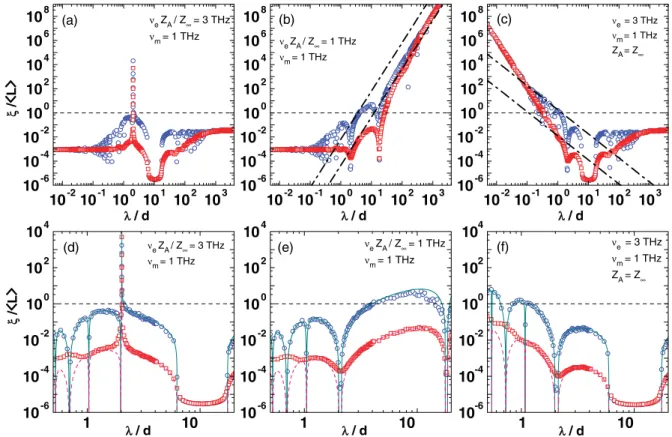
FIG. 3. (Color online) Localization length for normal incidence in units of the average system lengthLas a function of the vacuum wavelength (expressed in units ofd=a+b) forN=500 000 double layers in a RHM-LHM photonic system witha=b=12μm. LayersA
are composed by a nondispersive RHM, whereas in dispersive layersBboth the electric permittivity and magnetic permeability are described by a Drude-like model [cf. Eqs.(19)and(20), respectively]. Circles and squares correspond to numerical results obtained from Eq.(1)for=1μm and=12μm, respectively, and for 100 realizations of disorder. Calculations displayed in (a) and (b) were performed forǫ∞=1.21,μ∞=1, andǫA=μA=1 and correspond to the physical situations described in the first and third rows, respectively, of TableI. Results depicted in (c) are obtained forǫA=ǫ∞=1.21 andμA=μ∞=1 and correspond to Case 4 of TableI. In all cases, the corresponding plasmon frequencies νe=ωe/(2π) andνm=ωm/(2π) are given in each panel. Upper (=1μm) and lower (=12μm) oblique dashed-dotted lines depicted in panels (b) and (c) correspond, respectively, to theλ4andλ−2behaviors [cf. Eqs.(23)and(30), respectively]. Panels (d), (e), and (f) display the localization length, shown in panels (a), (b), and (c), respectively, in a short range of intermediate wavelengths, where solid and dashed curves are obtained from the I-M equation for=1μm and=12μm, respectively. Horizontal dashed lines represent the separation between localized and delocalized states.
layers A and B. Numerical results for ξ, in units of the average system length, are depicted in Fig. 3 as functions ofλfor normal incidence, forN =500 000 double layers in a RHM-LHM photonic system, and fora =b=12μm. Circles and squares correspond to numerical results obtained from Eq.(1)for=1μm and=12μm, respectively, and for 100 realizations of disorder. Calculations shown in Figs.3(a) and3(b)were performed for ǫ∞=1.21,μ∞=1, andǫA=
μA=1 (Z∞< ZA) and correspond to the physical situations
described in Cases 1 and 3 of Table I, respectively. Results shown in Fig. 3(c) were obtained for ǫA=ǫ∞=1.21 and
μA=μ∞=1 (Z∞=ZA) and for parameters taken according
to Case 4 of TableI. Upper (=1μm) and lower (=12 μm) dashed-dotted oblique lines depicted in Figs. 3(b) and 3(c)result from the asymptotic Eqs.(23)and(30), respectively. Horizontal dashed lines represent the border between localized and delocalized states. As one may note from Fig. 3, in all cases the I-M equation correctly predicts the critical-frequency values, i.e., a non-null and finite value ofωc(orλc=2π c/ωc)
in Fig.3(a),ωc=0 (λc→ ∞) in Fig. 3(b), and an infinite
value ofωc(λc=0) in Fig.3(c).
One should note that the numerical results represented by open symbols in Fig. 3(b) follow, in the long wavelength limit, the approximated expressionξ /L =∞(λ/d)α∞. The
values of ∞ and α∞ may be obtained for any value of the disorder amplitude by performing a statistical analysis. A detailed study of the results shown in Fig.3(b)leads to∞= (8.7±0.9)×10−5 and α
∞=4.06±0.03 for =1 μm,
whereas for =12 μm one obtains ∞=(7.2±0.6)× 10−5andα
∞=4.08±0.02. In spite that the I-M model is not
strictly applicable in the long wavelength limit, it is remarkable that the values ofα∞are found in good agreement with the λ4behavior predicted by Eq.(23). According to Eq.(23), the quantity equivalent to∞is∞/L, where∞is given by Eq.(24). We have straightforwardly obtained that∞/L = 6.4×10⁻³ and
∞/L =4.5×10⁻⁵ for =1 μm and
10-2 10-1 100 101 102 103 10-6
10-4 10-2 100 102
ν
e ZA / Z∞ = 1 THz
ν
m = 3 THz
ξ
/
L
λ
λ / d
FIG. 4. (Color online) Localization length for normal incidence, as in Fig.3(a), for plasmon frequencies νe=ωe/(2π) andνm=
ωm/(2π), which do not match any of the conditions of TableI.
numerical results of the localization length shown in Fig.3(c) may be approximated, in the short wavelength region, by the expressionξ /L =0(λ/d)α0. In this case we found0=
(1.27±0.08)×10−2andα0= −3.98±0.04 for=1μm,
whereas0=(1.16±0.05)×10−2andα0= −4.01±0.02
for =12 μm. Numerical results obtained from Eq. (1) suggest a dependenceξ ∝λ−4 of the localization length in
the limitλ→0. Such behavior differs quantitatively from the ξ ∝λ−2 dependence of the localization length predicted by the I-M equation [cf. Eq.(30)], a fact which is expected due to the divergence of both Q2AσA2 andQ2BσB2 as λ→0 and, therefore, to the inapplicability of Eq.(2)at this limit. Even though the description, by using Eq. (2), of the asymptotic behavior of the localization length in the limits of short and long wavelength is only qualitative in this particular case, such equation correctly predicts the values of critical frequencies. On the other hand, due to the particular frequency dependence of both ǫ(ω) and μ(ω) [cf. Eqs. (19) and (20)], one may note that the I-M may be used without difficulties in a finite window of the wavelength spectrum. In this sense, the good agreement between the I-M results and numerical calculations from Eq.(1)may be observed in Figs.3(d),3(e), and3(f).
We have depicted in Fig. 4 the localization length, for normal incidence, as a function of the vacuum wavelength. Both the electric and magnetic plasmon frequencies were chosen so that none of the conditions shown in Table Iare satisfied. The rest of parameters are the same as those used in Figs. 3(a) and 3(b). One may note that Z∞< ZA and
ωm> ωeZA/Z∞ in this case. According to Eq. (21), the
critical frequencyωcis an imaginary number in this case and,
as expected, the suppression of the Anderson localization is not observed.
In order to consider the effects of the oblique incidence on the localization length, we have investigated whether the behavior ofξ, obtained from the conditions of Fig.3, survives withθ =0. To this end, we depict in Figs. 5(a), 5(b), and 5(c) the localization length, as a function of the vacuum wavelength, calculated with the same sets of parameters as in Figs.3(a),3(b), and 3(c), respectively, for TE modes and incidence angleθ =π/3. Brewster anomalies at finite values of the vacuum wavelength may be clearly observed in all panels of Fig.5. Numerical values of such critical wavelengths (or frequencies) may be obtained by using the procedure described by Mogilevtsevet al..17One may note in Figs.5(d),5(e), and 5(f)the very good agreement, in a segment of the applicability region of Eq. (2), between the numerical results obtained from Eq. (1) and those obtained from the I-M equation. In contrast to the case of normal incidence in which Case 3 of TableIis satisfied [cf. Fig. 3(b)], the localization length does not diverge in the limit λ→ ∞ when θ =π/3 [cf. Fig. 5(b)]. Numerical results depicted in Fig. 5(b) indicate that the asymptotic behavior ofξ in the long wavelength limit is not robust for oblique incidence, i.e., it is strongly dependent on the incidence angleθ. Here we note that, when Case 4 of TableIis fulfilled, the diverging behavior of the localization length in the limitλ→0 still survives for oblique incidence, as one may note in Fig.5(c). This particular situation is due to the choice ofμA=μ∞=1 in the numerical calculations, as
we have mentioned in Sec.II. As a consequence, the function gOTEbecomes independent of θ in the short wavelength limit which, together with the conditionZA=Z∞, leads togTEO =0
asλ→0 and, therefore, to the suppression of the Anderson localization at this limit.
C. RHM-LHM superlattices with dispersive SRR responses Numerical results for the localization length in the long wavelength limit may not be reliable when the Drude-like model is used for the magnetic response of the metamaterial layersB. A more realistic model for describing the frequency dependence of the magnetic permeability of the slabs B is, therefore, advisable in order to study photonic-crystal properties in the low-frequency limit. We have then considered a split-ring resonator (SRR) response for the metamaterial slabsB, where the electric permittivity is still given by the Drude model [cf. Eq.(19)] and the magnetic permeability has the form30–32
μB(ω)=μ0
1−F ω
2
ω2−ω2 m
, (31)
where 0< F <1 is a factor which depends on the geometry of the split rings31andωmplays the role of a magnetic-resonance
frequency.
We now proceed, as in the above subsection, to find the critical frequencies from the I-M equation. For normal incidence the critical frequencies come from the condition gN(ωc)=0 and, therefore, are the real and positive solutions
of the equation
Z2
∞
ZA2 −1
ω4c+
ω2e+ω2m
1−Z
2
∞
Z2A 1 1−F
ω2c
10
-210
-110
010
110
210
310
-610
-410
-210
010
210
410
610
8λ
/ d
(c) νe= 3 THzνm = 1 THz
ZA = Z∞
1
10
10
-610
-410
-210
010
210
4 νe= 3 THz
νm = 1 THz Z
A = Z∞
(f)
λ
/ d
10
-210
-110
010
110
210
310
-610
-410
-210
010
210
410
610
8λ
/ d
(b) νe ZA / Z∞= 1 THz νm = 1 THz
1
10
10
-610
-410
-210
010
210
4νe ZA / Z∞= 1 THz
νm = 1 THz
(e)
λ
/ d
10
-210
-110
010
110
210
310
-610
-410
-210
010
210
410
610
8ξ
/
L
λ
/ d
(a) νe ZA / Z∞= 3 THz νm = 1 THz
1
10
10
-610
-410
-210
010
210
4νe ZA / Z∞= 3 THz
νm = 1 THz
(d)
ξ
/
L
λ
/ d
FIG. 5. (Color online) As in Fig.3but for TE modes and oblique incidence (θ=π/3). where ZA=√μA/√ǫA is the optical impedance of slabs
AandZ∞=√μ∞/√ǫ∞ is the optical impedance of meta-material layers B in the limit ω→ ∞. Here we note that μ∞=μ0(1−F) is the high-frequency magnetic permeability
of slabsB. The above equation, together with Eqs.(9)–(11), indicates thatω=0 is not a critical frequency and, therefore, we find localized states in the long wavelength limit.
For simplicity, we have studied the two particular cases of Eq.(32)which have been summarized in TableII. In Case 1 we have supposedZ∞=ZA, and as a consequence, the
fourth-order term inωcof Eq.(32)vanishes. One hasωe> ωm
F 1−F
in order to obtain real solutions forωc. The critical frequency
TABLE II. Two particular cases of Eq.(32). Conditions imposed to Eq. (32) guarantees the suppression of Anderson localization, for normal incidence, at the critical frequencies shown in the right column. The photonic system is composed by layersAof a nondispersive RHM, and by layersB of a SRR metamaterial with electric permittivity and magnetic permeability given by Eqs.(19) and(31), respectively.
Cases Conditions Critical frequency
1 ωe> ωm
F 1−F
Z∞=ZA
ωc→ ∞
ωc= ωeωm ω2
e−ω2m1−FF
2 ωe=ωm
Z2∞
Z2A(1−F)−1
Z∞> ZA
ωc=
√ω
eωm
4
Z2∞ Z2A−1
is then given by
ωc=
ωeωm
ω2 e−ω2m
F 1−F
. (33)
Also, due to the matching of the optical impedance of slabs AandB when ω→ ∞, one may expect the suppression of Anderson localization in such a limit. In this case, the behavior of the localization length, predicted from the I-M equation, is described by Eq.(26), where
Ŵ0=
32π2c4
ǫ2Aμ2
∞d
ω2 e−ωm2
F 1−F
2 (34)
andG0 =G0(λ) is given by Eq.(28), withμ∞=μ0(1−F)
in Eq.(29). The function modulating the maxima ofξis given by Eq.(30), with the appropriate value of0 obtained from
Ŵ0andG0, as we have mentioned in the above subsection.
In Case 2 of TableII, we have imposed the conditionωe=
ωm Z2
∞ Z2
A(1−F)−
1, with Z∞> ZA √
1−F in order to ωe be
real. As a consequence, the quadratic term inωcof Eq.(32)
vanishes, andZ∞> ZAfor obtaining real values of the critical
frequency. We have discarded the two imaginary solutions and the negative real solution of Eq.(32), as none of them has a physical meaning. The single positive solution forωcreads,
ωc= √ω
eωm
4
Z2
∞ Z2
A −1
. (35)
10-2 10-1 100 101 102
10-6
10-4
10-2
100
102
104
106
ξ
/
L
λ / d
(a)
10-2 10-1 100 101 102
10-6
10-4
10-2
100
102
104
106
ξ
/
L
λ / d
(b)
FIG. 6. (Color online) Localization length, for normal incidence, in units of the average system lengthL, as a function of the vacuum wavelength expressed in units of d=a+b. Calculations were performed using Eq. (1), a=b=12μm,N=500 000, and 100 realizations of disorder. Circles and squares correspond to numerical data obtained for =1 μm and =12 μm, respectively. The electric and magnetic responses of layersBare described by Eqs.(19) and(31), respectively, withǫA=ǫ∞=1.21,μA=1,F=1/4, and
ωe
2π =3 THz. Results displayed in (a) were computed by setting
μ0=4/3 andω2mπ
F
1−F =1 THz and correspond to Case 1 of TableII. Parameters used in (b) wereμ0=8/3 andω2πm
Z∞2 ZA2
1
1−F−1=3 THz and correspond to Case 2 of TableII. Upper and lower oblique lines in panel (a) correspond to the asymptotic behavior of the localization length, for =1μm and=12 μm, respectively, obtained as explained in the text. Horizontal dashed lines represent the separation between localized and delocalized states.
disorder amplitude for both slabs AandB. Figure 6 shows the normal-incidence localization length in a multilayered system with the electric and magnetic dispersions of slabsB given by Eqs.(19)and(31), respectively. Results depicted in Figs. 6(a) and 6(b) are obtained by appropriately choosing the superlattice parameters according to Cases 1 and 2, respectively, of Table II. Circles and squares correspond to =1 μm and =12 μm, respectively. As in the previous subsection, the localization length may be written, in the vicinity ofλ=0, asξ /L =0(λ/d)α0. A statistical
analysis of the numerical data obtained from Eq.(1)reveals that 0=(1.34±0.07)×10−2 andα0= −3.98±0.03 for
=1 μm, whereas 0=(1.08±0.04)×10−2 and α0= −4.03±0.02 for=12μm. Such results are in agreement with those previously obtained for the Drude-like response in metamaterial layersB and suggest a dependenceξ ∝λ−4
in the limitλ→0. The I-M equation correctly predicts the singularity of the localization length as λ→0, but such a prediction is only qualitative. For finite values of the critical frequency, however, the I-M equation quantitatively predicts the position of the peaks displayed in both Figs. 6(a) and 6(b). The corresponding vacuum wavelength (λc=2π c/ωc)
associated with those critical frequencies areλc/d ≈6.80 and
λc/d ≈4.73, respectively, and agree very well with the results
obtained from Eqs.(33)and(35), respectively.
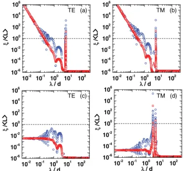
We have also numerically studied the influence of oblique incidence on the localization length. Results computed from Eq. (1) are displayed in Fig. 7. In panels7(a) and 7(b)we have used the same set of parameters of Fig.6(a), whereas in panels 7(c) and 7(d) the corresponding parameters were
10-2 10-1 100 101 102 10-6
10-4 10-2 100 102 104 106
ξ
/
L
λ / d
TE (a)
10-2 10-1 100 101 102 10-6
10-4 10-2 100 102 104 106
ξ
/
L
λ / d
TM (b)
10-2 10-1 100 101 102 10-6
10-4 10-2 100 102 104 106
ξ
/
L
λ / d
TE (c)
10-2 10-1 100 101 102 10-6
10-4 10-2 100 102 104 106
ξ
/
L
λ / d TM (d)
FIG. 7. (Color online) TE and TM localization lengths, in units of the average system lengthL, for oblique incidence withθ=π/3. Results depicted in (a) and (b) were performed for the same set of parameters used in Fig.6(a), whereas the data plotted in (c) and (d) are evaluated using the parameters of Fig.6(b). Horizontal dashed lines represent the separation between localized and delocalized states.
chosen as in Fig.6(b). Calculations shown in Figs.7(a)and 7(c)[7(b)and7(d)] were obtained for TE (TM) modes. It is apparent from Figs.7(a)and7(b)that the singularity ofξ in the limitλ→0 still survives in the case of oblique incidence for both the TE and TM modes. As discussed above, these facts are due to the choice of μA=μ∞=μ0(1−F) and
ǫA=ǫ∞together with the matching of the optical impedances
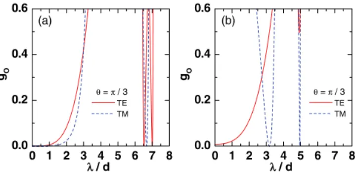
of the slabs A andB in the high-frequency limit. In other words, the delocalization in the limitλ→0 is omnidirectional for the photonic superlattice studied in Figs.6(a),7(a), and 7(b). Moreover, all the singularities of the localization length appearing for positive finite values ofλcorrespond to Brewster anomalies. As one may note from Fig.7(c) for TE modes, the oblique incidence may lead to a situation in which no suppression of the Anderson localization is observed in the whole range of wavelengths considered in the present study. As mentioned before, the positions of the singularities of ξ in the frequency (or wavelength) spectrum for both TE and TM modes in the case of oblique incidence may be fully understood by analyzing the functions gOTE and gOTM, respectively [cf. Eqs. (15) and (16), respectively], which are displayed in Fig. 8 for the different cases depicted in Fig.7. For example, for the TE modes shown in Fig. 7(a) the corresponding function gOTE, represented as a solid line in Fig.8(a), vanishes atλc/d =0,λc/d ≈6.525, andλc/d ≈
7.007. The two last values ofλcare a doublet which is observed
in Fig.7 (a), due to the scale of the figure, as a single peak in the localization length. For the TM modes in Fig. 7(b) we have two singularities corresponding to the zeros ofgOTM [cf. dashed line in Fig.8(a)] located atλc/d =0 andλc/d ≈
0 1 2 3 4 5 6 7 8 0.0
0.2 0.4 0.6
θ = π / 3 TE TM
gO
λ / d (a)
0 1 2 3 4 5 6 7 8 0.0
0.2 0.4 0.6
θ = π / 3 TE TM
gO
λ / d (b)
FIG. 8. (Color online) Vacuum wavelength dependence of func-tionsgX
Oforθ=π/3. Solid and dashed lines correspond toX=TE and X=TM electromagnetic modes, respectively [cf. Eqs. (15) and (16), respectively]. Results displayed in panel (a) correspond to the first case of TableIIwith parameters used in Figs.7(a)and 7(b), whereas in panel (b) we use the set of parameters of Figs.7(c) and7(d), which correspond to the second case of TableII.
[see the solid line in Fig.8(b)], corresponding to the TE modes displayed in Fig.7(c), does not vanish atλ=0 or at other values of λ and, therefore, the TE modes remain localized in this case. Also, the TM modes displayed in Fig.7(d)are delocalized atλc/d ≈3.179 andλc/d ≈4.948, which are the
zeros of the corresponding function gTMO [cf. dashed line in Fig.8(b)].
D. Absorption effects
As metamaterials are intrinsically dispersive materials, it is also convenient to investigate the effects of absorption on the localization length. Such effects may be appropriately introduced by modifying the electric and magnetic responses of the heterostructure slabs. Here we assume that slabsAare nondispersive, whereas the electric susceptibility of slabsBis given by
ǫB(ω)=ǫ∞
1− ω
2 e
ω(ω+i ωeγe)
, (36)
where γe is a phenomenological electric damping constant
expressed in units of the electric plasmon frequency. Within the Drude-like model the magnetic permeability of the slabs
Bis given by
μB(ω)=μ∞
1− ω
2 m
ω(ω+i ωmγm)
, (37)
where γm is the magnetic damping constant in units of the
magnetic plasmon frequency. Numerical calculations for the localization length may then be obtained from Eq.(1).
To illustrate absorption effects onξ, we depict in Fig. 9 the localization length for normal incidence, as a function of λ, and for various values of the electric and magnetic damping constants. Calculations displayed in Figs.9(a),9(b), and9(c)were performed for the same set of parameters used in Figs.3(a),3(b), and3(c), respectively. Here we have restricted the range ofλ to a vicinity of the critical frequencies. It is apparent from Fig.9(a)that the Brewster anomaly, obtained in the absence of absorption, becomes smeared out as the damping constants increase. This is related to the decrease of the intensity of the transmitted beam due to the absorption in the metamaterial layers. Moreover, the asymptotic behavior of the localization length in the limit λ→ ∞ observed in Fig. 9(b) for γe=γm=0 is dramatically modified in the
presence of the absorption. In this case, numerical calculations indicate that the λ4 behavior of ξ does not survive when
the damping constants are introduced. Results in Fig.9(c), however, indicate that the divergence ofξ in the limitλ→0 still remains in the presence of absorption.
IV. CONCLUSIONS
Summing up, we have investigated the localization prop-erties of electromagnetic waves in 1D disordered photonic superlattices in which the electric permittivity and magnetic permeability of the different slabs composing the heterostruc-ture may depend on the wave frequency. First, we have per-formed a theoretical study of the properties of the localization length by using the I-M model recently developed for weakly disordered photonic systems.17,22 In addition, we carried out numerical calculations of the localization length by using its definition [cf. Eq. (1)] involving the transmissivity of the heterostructure. Generally speaking, the I-M results for the localization length agree with the numerical results obtained from Eq.(1)only for small amplitudes of disorder, and in a
10-2 10-1
10-2
100
102
104
106
108
λ / d
(c)
νe= 3 THz
νm = 1 THz ZA = Z∞
102 103
10-8
10-4
100
104
108
λ / d
(b)
νe ZA / Z∞= 1 THz
νm = 1 THz
100 101
10-6
10-4
10-2
100
102
104
ξ
/
L
λ / d
(a)
νe ZA / Z∞= 3 THz
νm = 1 THz
FIG. 9. (Color online) As in Fig.3, with=1μm, and including effects of the absorption on the localization length. Results were displayed in the vicinity of a critical frequency. Squares, circles, up-triangles, and down-triangles correspond to damping constants γe=γm=0,
region of the frequency spectrum where the I-M model is valid. Such a region is determined by the frequency dependence of both the electric permitivitty and magnetic permeability of the materials composing the heterostructure. In all cases studied in the present work, the I-M equation correctly predicts the critical-frequency values at which the localization length diverges and suppression of Anderson localization occurs.
For nondispersive RHM-RHM superlattices, present nu-merical results confirm theλ2dependence of the localization
lengthξin the long wavelength limit, whereas for LHM-RHM photonic crystals we have shown that the asymptotic behavior of the localization length is strongly dependent on both electric and magnetic responses that characterize the LHM slabs, i.e., it is essentially determined by the specific type of metamaterial which constitutes the LHM layers. In this sense, results obtained from Eq. (1) suggest, under certain conditions discussed in Sec. III, a λ4 dependence of the localization length, only for normal incidence, in the limit λ→ ∞. Moreover, in some specific cases the localization length exhibits aλ−4asymptotic behavior asλ
→0, which is
observed for both normal and oblique incidence and even in the presence of absorption.
Here, one should point out that researchers worldwide are making efforts to develop fabrication techniques that compensate losses to produce more efficient photonic media.33 Therefore, the combination of metamaterials with electrically and optically pumped gain media and emerging graphene technology is expected to lead to low-loss materials suitable to use in optical devices and in the electronics industry. In that respect, we do hope the present theoretical study will help to stimulate low-loss experimental studies and further experimental and theoretical work on the subject of suppression of Anderson localization in disordered photonic heterostructures.
ACKNOWLEDGMENTS
The present work was partially financed by Brazilian Agencies CNPq and FAPESP as well as by the Scientific Colombian Agency CODI, University of Antioquia.
1P. W. Anderson.Phys. Rev.109, 1492 (1958).
2A. Lagendijk, B. A. van Tiggelen, and D. S. Wiersma,Phys. Today
62, 24 (2009).
3S. John,Phys. Rev. Lett.58, 2486 (1987). 4S. F. Liew and H. Cao,J. Opt.12, 024011 (2010).
5J. D. Joannopoulos, S. G. Johnson, J. N. Winn, and R. D. Meade, in Photonic Crystals: Molding the Flow of Light(Princeton University Press, Princeton, 2008).
6D. R. Smith, W. J. Padilla, D. C. Vier, S. C. Nemat-Nasser, and S. Schultz,Phys. Rev. Lett.84, 4184 (2000).
7P. Markoˇs and C. M. Soukoulis,Wave Propagation: From Elec-trons to Photonic Crystals and Left-Handed Materials(Princeton University Press, Princeton, 2008).
8C. Enkrich, M. Wegener, S. Linden, S. Burger, L. Zschiedrich, F. Schmidt, J. F. Zhou, Th. Koschny, and C. M. Soukoulis,Phys. Rev. Lett.95, 203901 (2005).
9W. Cai, U. K. Chettiar, H. K. Yuan, V. C. de Silva, A. V. Kildishe, V. P. Drachev, and V. M. Shalaev,Opt. Express15, 3333 (2007). 10D. R. Smith, J. B. Pendry, and M. C. K. Wiltshire,Science305, 788
(2004).
11J. B. Pendry, D. Shurig, and D. R. Smith, Science 312, 1780 (2006).
12U. Leonhardt,Science312, 1777 (2006).
13A. A. Asatryan, L. C. Botten, M. A. Byrne, V. D. Freilikher, S. A. Gredeskul, I. V. Shadrivov, R. C. McPhedran, and Y. S. Kivshar, Phys. Rev. Lett.99, 193902 (2007).
14A. A. Asatryan, S. A. Gredeskul, L. C. Botten, M. A. Byrne, V. D. Freilikher, I. V. Shadrivov, R. C. McPhedran, and Y. S. Kivshar, Phys. Rev. B81, 075124 (2010).
15P. Sheng, Introduction to Wave Scattering, Localization, and Mesoscopic Phenomena(Academic, New York, 1995).
16E. J. Torres-Herrera, F. M. Izrailev, and N. M. Makarov,Europhys. Lett.98, 27003 (2012).
17D. Mogilevtsev, F. A. Pinheiro, R. R. dos Santos, S. B. Cavalcanti, and L. E. Oliveira,Phys. Rev. B82, 081105(R) (2010).
18D. Mogilevtsev, F. A. Pinheiro, R. R. dos Santos, S. B. Cavalcanti, and L. E. Oliveira,Phys. Rev. B84, 094204 (2011).
19E. Reyes-G´omez, A. Bruno-Alfonso, S. B. Cavalcanti, and L. E. Oliveira,Phys. Rev. E84, 036604 (2011).
20A. A. Asatryan, L. C. Botten, M. A. Byrne, V. D. Freilikher, S. A. Gredeskul, I. V. Shadrivov, R. C. McPhedran, and Y. S. Kivshar, Phys. Rev. B85, 045122 (2012).
21J. E. Sipe, P. Sheng, B. S. White, and M. H. Cohen,Phys. Rev. Lett.
60, 108 (1988).
22F. M. Izrailev and N. M. Makarov,Phys. Rev. Lett.102, 203901 (2009).
23M. M. Sigalas, C. M. Soukoulis, C. T. Chan, R. Biswas, and K. M. Ho,Phys. Rev. B59, 12767 (1999).
24L. I. Deych, D. Zaslavsky, and A. A. Lisyansky,Phys. Rev. Lett.
81, 5390 (1998).
25Cheng-Ching Wang, and Pi-Gang Luan,Phys. Rev. E65, 066602 (2002).
26M. Mazilu and K. Dholakia,Opt. Express14, 7709 (2006). 27Sadao Adachi,J. Appl. Phys.58, 1R (1985).
28H. Jiang, H. Chen, H. Li, Y. Zhang, and S. Zhu,Appl. Phys. Lett.
83, 5386 (2003), and references therein.
29L. H. Zhang, Y. H. Lia, Y. Q. Ding, W. Tan, H. T. Jiang, Z. G. Wang, H. Q. Li, Y. W. Zhang, and H. Chen,Eur. Phys. J. B77, 1 (2010). 30T. J. Yen, W. J. Padilla, N. Fang, D. C. Vier, D. R. Smith, J. B.
Pendry, D. N. Basov, and X. Zhang,Science303, 1494 (2004). 31F. S. S. Rosa, D. A. R. Dalvit, and P. W. Milonni,Phys. Rev. Lett.
100, 183602 (2008).
32R. S. Penciu, M. Kafesaki, Th. Koschny, E. N. Economou, and C. M. Soukoulis,Phys. Rev. B81, 235111 (2010).

![TABLE I. Conditions for which ω c [cf. Eq. (21)] is a critical frequency, obtained for photonic systems composed by layers A of a nondispersive RHM and LHM layers B with dispersives electric permittivity and magnetic permeability given by a Drude-like mode](https://thumb-eu.123doks.com/thumbv2/123dok_br/16300349.186049/6.911.538.835.119.235/conditions-critical-frequency-nondispersive-dispersives-permittivity-magnetic-permeability.webp)