3D Reconstruction of Coronary Artery
Vascular Smooth Muscle Cells
Tong Luo1, Huan Chen1, Ghassan S. Kassab1,2,3*
1Biomedical Engineering, IUPUI, Indianapolis, IN, United States of America,2Surgery, IUPUI, Indianapolis, IN, United States of America,3Cellular and Integrative Physiology, IUPUI, Indianapolis, IN, United States of America
Abstract
Aims
The 3D geometry of individual vascular smooth muscle cells (VSMCs), which are essential for understanding the mechanical function of blood vessels, are currently not available. This paper introduces a new 3D segmentation algorithm to determine VSMC morphology and orientation.
Methods and Results
A total of 112 VSMCs from six porcine coronary arteries were used in the analysis. A 3D semi-automatic segmentation method was developed to reconstruct individual VSMCs from cell clumps as well as to extract the 3D geometry of VSMCs. A new edge blocking model was introduced to recognize cell boundary while an edge growing was developed for opti-mal interpolation and edge verification. The proposed methods were designed based on Region of Interest (ROI) selected by user and interactive responses of limited key edges. Enhanced cell boundary features were used to construct the cell’s initial boundary for further edge growing. A unified framework of morphological parameters (dimensions and orienta-tions) was proposed for the 3D volume data. Virtual phantom was designed to validate the tilt angle measurements, while other parameters extracted from 3D segmentations were compared with manual measurements to assess the accuracy of the algorithm. The length, width and thickness of VSMCs were 62.9±14.9μm, 4.6±0.6μm and 6.2±1.8μm (mean±SD).
In longitudinal-circumferential plane of blood vessel, VSMCs align off the circumferential direction with two mean angles of -19.4±9.3° and 10.9±4.7°, while an out-of-plane angle (i.e., radial tilt angle) was found to be 8±7.6° with median as 5.7°.
Conclusions
A 3D segmentation algorithm was developed to reconstruct individual VSMCs of blood ves-sel walls based on optical image stacks. The results were validated by a virtual phantom and manual measurement. The obtained 3D geometries can be utilized in mathematical models and leads a better understanding of vascular mechanical properties and function. OPEN ACCESS
Citation:Luo T, Chen H, Kassab GS (2016) 3D Reconstruction of Coronary Artery Vascular Smooth Muscle Cells. PLoS ONE 11(2): e0147272. doi:10.1371/journal.pone.0147272
Editor:Thomas Abraham, Pennsylvania State Hershey College of Medicine, UNITED STATES
Received:December 29, 2014
Accepted:January 2, 2016
Published:February 16, 2016
Copyright:© 2016 Luo et al. This is an open access article distributed under the terms of theCreative Commons Attribution License, which permits unrestricted use, distribution, and reproduction in any medium, provided the original author and source are credited.
Data Availability Statement:All relevant data are within the paper and its Supporting Information file.
Funding:This work was supported by the National Institute of Health-National Heart, Lung, and Blood Institute Grant 1 R01 HL117990.
Introduction
Mechanical stresses induced in the vessel wall are in part influenced by arrangement and shape of individual vascular smooth muscle cells (VSMCs), most of which are believed to be mainly distributed along the circumference of the vascular wall [1–3]. There has been significant effort, based on 2D histology images [4], to determine cellular morphology to predict vascular mechanical response. The mechanical models, however, require accurate geometrical informa-tion of cells exposed to the biomechanical microenvironments of vessel wall [5–6]. It is expected that 3D cellular structure can provide more accurate geometries (e.g., 3D dimensions and orientation) for better understanding of vascular biomechanics. Furthermore, realistic 3D cellular morphology of blood vessels are also essential for understanding pathology of blood vessels, given that the major causes of cardiovascular disease (e.g., hypertension and atheroscle-rosis) typically involve hypertrophy or hyperplasia of VSMCs [7–8]. A 2D view of cells is lim-ited and complex geometric features can be more accurately represented based on 3D
reconstruction of cells. The latest developments of microscopy technology enable noninvasive visualization of VSMCs [9] and provides high-quality image stacks for computational analysis of 3D reconstruction of individual cells.
A complete VSMC reconstruction requires 3D cell segmentation and surface coordinates [10]. Generally, the studies of 3D model reconstruction have focused on single cells in clumps. Complex and tenuous structure of multiple cells, however, challenge most image analysis methods. Some new algorithms address special VSMCs clump segmentation [11–12], while most 3D models have been reduced to simple geometries and were not segmented from cell samples [13]. An efficient segmentation algorithm is needed to improve accuracy of 3D recon-struction for a single cell.
There exist two main problems in VSMC segmentations: 1) the general segmentation prob-lem must be solved and 2) the special features of VSMC scanned in longitudinal-circumferen-tial plane must be captured. The major challenge is to distinguish boundaries of touching or overlapped objects [14–17]. The limitation of segmentation algorithms in microscope images has been discussed in the literature [17–18], and there are inter-cell and intra-cell intensity var-iances (intersection of grey levels among different objects), such as adjacent cells and back-ground. Generally, weak boundaries typically occur in object neighboring. Specifically, cell clumps containing multiple cells with various shapes, sizes, orientations and positions, make complex structures that are difficult to analyze.
Here, we analyzed the geometry and shape of VSMCs by introducing a new edge blocking model for cell clump segmentation algorithm. The cell edge was decomposed into several parts and different strategies were tested. Edge stability and edge growing were proposed to address the edge gap problem. A virtual phantom model was used to validate the measurements of VSMC tilt angles, while the validation of other parameters was made by comparison with man-ual measurements. The 3D geometries of VSMCs including the width, length, thickness, slen-derness ratio, in-plane angle (orientation in longitudinal-circumferential plane) and out-of-plane angle (i.e., radial tilt angles) were extracted based on the 3D reconstruction.
Methods
VSMC Image Data
Images from six healthy pig (body weight in the range of 80–90 Kg) coronary arteries were ana-lyzed in the present study. The hearts were harvested immediately after sacrifice at a local slaughterhouse (Archers Meats, Greenwood, IN; where our group was located when the mea-surements were performed). Details have been provided in a previous study [19]. The hearts
were then transported to the laboratory in 4°C physiological solution (0.9% NaCl) and the cor-onary artery segments were dissected carefully from the hearts and immersion-fixed in 4% methanol-free paraformaldehyde solution. 5x5 mm2cross-sections were then sectioned from the segments and the circumferential direction was marked (Fig 1a). The adventitia was peeled off from the sections to facilitate the staining and imaging, and samples were then labeled by two fluorescent probes: phalloidin (excitation/emission wavelength: 495/518 nm) and DAPI (excitation/emission wavelength: 358/461 nm) to capture the F-actin and nucleus of VSMCs (Fig 1b). After staining, the sections were wet mounted on microscope slides using a glycerin-water mixture. The samples were scanned by an FV1000-MPE confocal microscope equipped with multiple laser options and a 60x 1.1NA water immersion objective. Z-stack scans were performed with a 0.25μm step size, and a scanning spot (i.e., imaging data set) covered a vol-ume of 211x211x10μm3.
User Input
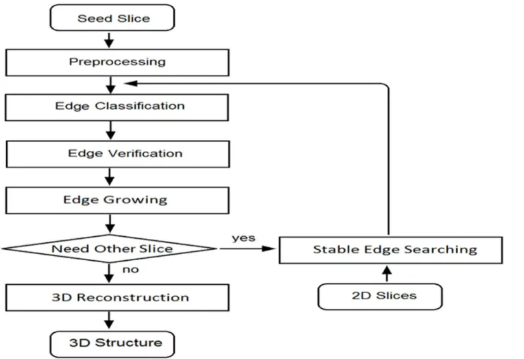
An ROI on initial slice was drawn by a user in the semi-automation segmentation algorithm. Specific nuclei were selected to be the start points, and edges in ROI were processed and treated as initial edges. A flow chart for image processing is shown inFig 2where the primary proce-dures are introduced in the paragraphs below and the algorithm technical details are presented inS1 Fig. In sequential slices, edges were detected by a newly developed edge blocking method. The edge blocking method may lead to false results under some circumstances, however, such as when some edges overlap with others. Hence, user input was needed to select initial slice or key edges. Slice numbers were selected based on average nucleus thickness. Generally, 13–15 Fig 1. a)Vessel were imaged (black dot region) on longitudinal-circumferential plane. X, Y, and Z indicate the longitudinal direction, circumferential directions and radial directions of blood vessel, respectively;b)
Image with a resolution of 512 × 512 pixels. Blue indicates the nucleus, and green indicates F-actin, i.e., the cell.
slices were used for a nucleus. Usually, the 2D boundary was composed of dozens of points, manual segmentation cannot have the enough high accuracy and all boundary points were used to sketch out boundary. The computerized gap linking method operated directly on edge segments which were points groups, the time complexity of computerized method is roughlyO (N)on part of boundary points where the edge detection is revised.
Output Definition
The output of original images was the cell contours in 2D slices and 3D object. The 3D segmen-tation of entire cell including nucleus and cytoskeletal structures. Based on 2D contours, the 3D object was reconstructed, and smooth surface was obtained for further geometric measure-ments. The 3D nucleus structure was obtained from nucleus image and used for tilt angle mea-surements. More details of geometrical parameter extractions are outlined below. The
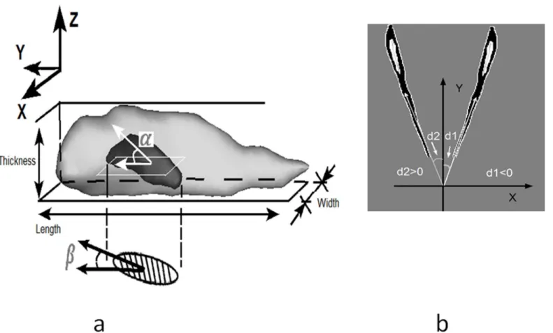
schematic definition of the parameters of VSMC length, width and thickness are illustrated in Fig 3awhere the actual 3D shape of the nucleus is presented.
Extraction of Geometrical Parameters
Out-of-plane and In-plane orientation angles are shown asαandβinFig 3a. The projection of a 3D cell on the XY plane (i.e., longitudinal-circumferential plane) approximates an ellipse that Fig 2. Flow chart of the image processing algorithm.
doi:10.1371/journal.pone.0147272.g002
consists of a long axis and a short axis by using a MATLAB Function RegionProps. According to spherical coordinate system terminology, in-plane angle is an angle between the long axis and the Y direction (i.e., circumferential direction of the vessel), while out-of-plane angle is an altitude angle out of XY plane. Orientation was also pointed towards the cell blunt pole and there was a deviation from the Y-axis in 2D image coordinates. The in-plane orientation angle was then outputted and ranges from -90 to 90 degree (the circumferential direction is defined as 0) as shown inFig 3b. The thickness was extracted on height along Z axis; and the length and width were extracted based on 2D projections.
To measure the tilt angle (defined in the range of 0 to 90°), the 3D surface coordinates of cell were used to form 3-by-3 covariance matrix, which measures the position difference between XYZ directions. A Principal component analysis (PCA) was employed to obtain the principal component vector that was equal to the tilt direction. A PCACOV function in MATLAB can be used for the analysis with two options: normalized coordinates with data size or non-normalized coordinates. The accuracy of two options was analyzed inS1 Fig. The tilt angle was extracted based on the nucleus image based on the same approach.
Edge Blocking Model
An idealized shape model of a single cell is shown inFig 4a. Longitudinal-circumferential plane was denoted asY-Xplane. The nucleus was binarized and overlapped virtually to the cell Fig 3. a) 3D surface rendering of nucleus denotes the out-of-plane angle (tilt angle), labeled asα, in-plane orientation angle of projected nucleus was denoted asβ. Shade region below in XY plane is an approximate ellipse for nucleus region. X,Y,Z coordinate axis is consistent with that inFig 1. The definition of cell length, width and thickness were illustrated.b)Two cell with typical in-plane angles were illustrated.
image (i.e., image of F-actin) at the cell center. Outside the nucleus, the edges or segments sym-metrically distributed and the boundary was defined as:
cell boundary¼ fleftðrightÞtrunk edge;leftðrightÞ tail edge;gapg ð1Þ
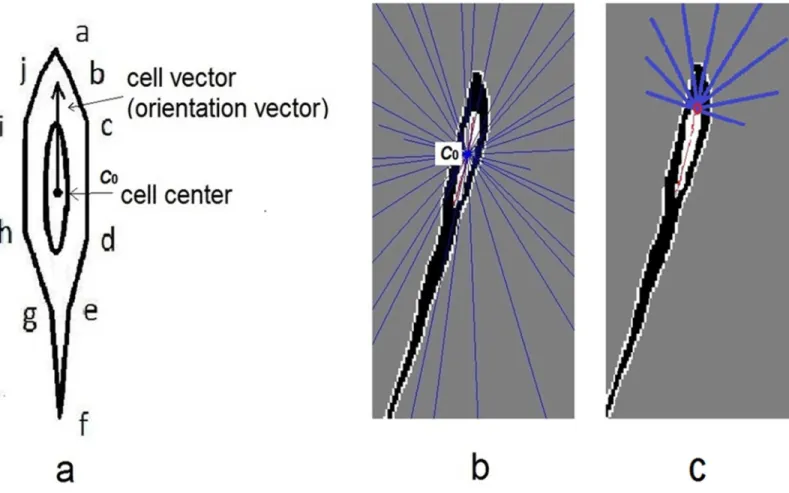
The left and right trunk edges were relatively close to the nucleus. Since a cell has varying curvature and width, the inner edges were detected in a cell image in which the intensity was lower in the nucleus region. Nuclei center pixel was defined as the cell center. Each cell was also equalized to a cell vector (orientation vector) from center to one endpoint of long axis. After nucleus region thinning, one skeleton with two end points was extracted by Matlab R2011b Image Processing toolbox function BWMORPH. The function provided specific math-ematical morphology operations to the binary image, such as regional thinning and finding endpoint.
An edge blocking model was proposed such that the cell edge segments were intersected by ray lines emitted from centerc0. A cell image with ray lines is illustrated inFig 4b, in which nucleus skeleton is depicted in red and the blue lines are ray lines. The first intersection points were determined by the cellular edge and ray lines. Edges of adjacent cells and ray lines may also intersect, but their intersections were considered to be blocked by current cell edge. The Fig 4. a)An idealized shape model of single cell was showed. The right edge was ordered in a-b-c-d-e-f. A trunk edge was b-c-d-e and tail edge was a-b and e-f. The cell center was overlapped by ellipses, it was the nucleus. A vector of the cell direction is indicated by an arrow along the long-axis of the cell. Cell center was denoted as C0.b)Blue ray lines emitted from the center, while the nucleus skeleton in red was drawn with two end points.c)Extended ray lines were emitted from end point.
doi:10.1371/journal.pone.0147272.g004
ray line is defined as a vector, emitted from the geometric center of the nucleus. The two fea-tures in ray include scattering angleθand emitting lengthlfrom the center to intersection
point. The angleθwill be converted from radian into degree within range of [0−360°) as
fol-lows:
y¼mod ðtan 1 ny
nx
tan 1 y y0 x x0
Þ; 6:28
ð2Þ
l¼lc0ð1þlc1cosðyÞÞ; lc1¼5;lc0 ¼30 ð3Þ
where (nx,ny) denotes cell vector, (x,y) denotes edge point and (x0,y0) denotes cell center. The length unit is pixel andlc1,lc0are determined as the minimal and maximal emitting lengths, respectively. If the ray lines are parallel to edge direction at the tail, new expanded ray lines are emitted from the one end point of skeleton to increase scattering area (Fig 4c).
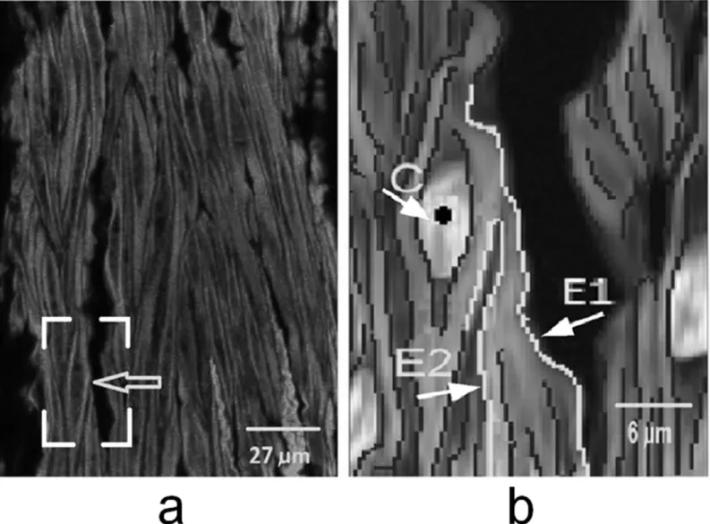
There are two kinds of edge gaps in a cell: 1) Type I is gaps between broken edges of the same cell, and 2) Type II is caused by other cells overlapping or adhering (as shown inFig 5; Fig 5ais the original image, andFig 5bis a zoom-in image. E1, E2 are edges of two different cells. Generally, when ray line is emitting from the center pointC, some parts of E1 and E2 are blocked by cell edge centered at pointC. Gaps were detected based on the edge blocking model and only unblocked segments were retained and linked later. In this model, block detection was implemented by intersections of rays and edges [20], and it is efficient for segmentation of various shape objects.
2D to 3D Segmentation
Cell edges were first processed by using the edge blocking model. The ray lines intersect with three types of edges: inner edge, Type A/B/C edge, or edge of other cells as defined inS1 Fig. The intersection pointes can be ordered according to their distance to the center; i.e., the closest are the first points, and the farthest are the third points. The third points were usually blocked by the first two and treated as noises. The inner edge was connected to the nucleus region and removed by region growing. After the gap type was identified, the corresponding gap can be filled by either Bilateral Spline Interpolation or Laplace verification principal component anal-ysis (PCA).
Anisotropic filtering was done in preprocessing and edge growing was based on different edge category. Edge feature was enhanced by edge verification. The edge in 3D context was searched based on stable edge criteria, where the stable edge was obtained in 2D slices. The seg-mentations were implemented based on sequential 2D images of cells where adjacent slices pro-vide 3D structural information. The challenge is cell segmentation due to the complex structure, while the segmentation of the nucleus is relatively easy and can be completed by ImageJ process binary toolbox. The 2D boundary of a slice was acquired after edge linking, and then used for 3D segmentation. The 3D surface was rendered by overlapping and filling 2D boundaries of all sequential slices. The MATLAB mathematical morphological operation function of BWMORPH was used to fill gaps and remove noise from binary images. MeshLab was a software tool used to improve the quality of generated 3D mesh and Meshlab global Laplacian smooth was used for initial smoothing and selected face smooth was used to refine the local geometry.
Validation of Tilt Angle Measurement
angles are predefined. The surface mesh was converted into sequential 2D images, which were later reconstructed into the 3D object using the proposed 3D algorithm. The tilt angle was extracted based on the reconstructed 3D ellipsoid and compared with the predefined angle.
Manual Validation of 2D Morphology Parameters
Manual validation is a typical method used in computer segmentation when there is no gold stan-dard [19]. Manual geometry measurements of the same cells on 2D images were performed by a different person (blinded to the automated results) by use of ImageJ to validate the proposed 3D algorithm. A 2D image slice (usually in the middle of a stack) was selected to present 2D geometry of individual cells. The length, width, slenderness ratio (defined as length/width) and in-plane ori-entation angle of cells were measured directly on 2D images and then compared with the semi-automatic measurements. ImageJ provides measurement toolbox for manual operations. To reduce noise, width was obtained by taking the average of measurements at several positions. The validation was based on statistical results and the mean and variances were compared.
Fig 5. a)Original image, arrow indicates the position of Fig 5b. The nuclei were in darker gray and overlaid from separated image. Cell was in gray.b)Zoom in region from box frame in Fig 5a, where E1, E2 were edges from two merged cells, and dark dot C was a cell center.
doi:10.1371/journal.pone.0147272.g005
Results
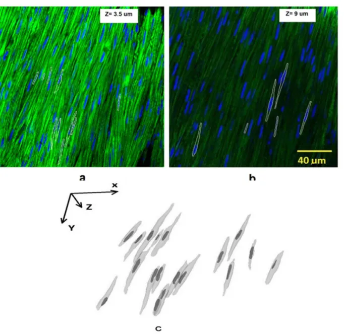
The original cell image and overlapped segmentation contours are shown inFig 6a and 6b. Two slices were used to depict the contours of 3D object (the depths at z direction were 3.5 and 9μm, respectively). The 3D structure of VSMCs is rendered inFig 6cwhere the X, Y, Z coordi-nates align with that of the 2D image. The longitudinal and circumferential directions of vessel segment correspond to X and Y axis, respectively; when the radial direction corresponds to the Z direction inFig 6c. Eighteen cells including the nuclei were reconstructed. Although some cells were very close to adjacent cells, they were distinguished by their respective nuclei (dark color). Since the largest contour of each cell was not always in the same plane, the contour sizes of cells were different.
Fig 6. a)3D cell contours in white were overlapped on original cell image. A slice at z = 3.5μm was analyzed. Blue indicates the nucleus, and green indicates the cell.b)A different slice at z = 9μm was analyzed to depict various layers of contours.c)3D rendering of cells and nuclei from a representative sample. The XYZ Coordinate system was consistent with that inFig 1. The viewpoint was taken from bottom to top along Z axis.
The statistical distributions of morphometry of 112 VSMCs are shown inFig 7a–7dfor length, width, thickness, and orientation angle, respectively. The length, width and thickness (Fig 7a–7c) show approximately normal distributions with mean±SD of 62.9±14.9μm, 4.6 ±0.6μm and 6.2±1.8μm, respectively, while the in-plane orientation distribution (Fig 7d) is a bimodal normal distribution (mixture of two normal distributions) with two different mean angles of -19.4±9.3° and 10.9±4.7°. The analysis of out-of-plane angles was based on more than 1,600 nuclei which shows a skewed distribution with a mean angle of 8.0±7.6° (median of 5.7°) (Fig 7e). Our results show that most VSMCs align off the circumferential direction with two nearly symmetric in-plane angels and with a small out-of-plane angle.
The geometrical parameters and orientation of VSMCs obtained by both the semi-auto-mated method and manual measurements are summarized inTable 1. There was excellent agreement between segmentation algorithm and manual measurements. Measurements of Fig 7. Various geometric parameters and orientation from cells:a)Length (μm).b)Width (μm);c)Thickness (μm),d)Orientation (degree) had two different values.e)Out-of-plane angle (degrees) histogram analyzed based on more than 1600 nuclei. Mean is the average value of measurement and SD is the standard variance. The normal distribution curve were fitted in the histograms in Fig 7a–7d, kernel distribution curve was fitted in Fig 7e.
doi:10.1371/journal.pone.0147272.g007
orientation angle were nearly identical for both methods, while the difference between mea-surements of length and width were 2.7% and 4.7%, respectively. The comparison of intra-group measurements was summarized in Tables2–4. If there was bimodal distribution of in-plane orientation angle in each heart, the comparison was listed in two columns inTable 3. Results show that the difference was<10% for most parameters.
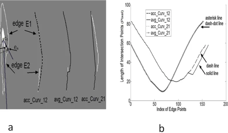
For the interpolation procedure, we proposed a new algorithm of Bilateral Spline Interpola-tion (details are outlined inS1 Fig). An example is illustrated inFig 8to compare the measure-ment of accumulated curvature (acc_Curv) to average curvature (avg_Curv). The two circles (as noted by arrows e2jand e1i) in the left cell ofFig 8awere unblocked and blocked intersection points, respectively. The three right columns inFig 8awere the interpolated new edges (dark line), acc_Curv_12 means from edge 2 to edge 1. Different edge sequences and measurement Table 1. Geometric data of vascular smooth muscle cells.
Number Orientation (degrees) Length (μm) Width (μm) Thickness (μm) Slenderness Ratio
Algorithm (n = 112) -19.4±9.3 62.9±14.9 4.6±0.6 6.2±1.8 12.3±4.3
10.1±4.7
Manual (n = 112) -19.2±9.2 61.2±14.1 4.4±0.7 14.1±3.3
11.1±4.3
Orientation is the binary 2D region orientation projected from 3D data. Length and Width were computed on the 2D region. The values are summarized as average and standard deviation (mean±SD). The second row was the manual measurement result in 2D images.
doi:10.1371/journal.pone.0147272.t001
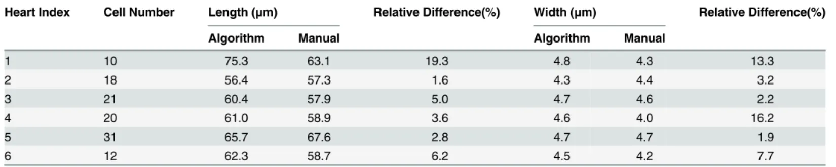
Table 2. Geometric data measurement by each heart.
Heart Index Cell Number Length (μm) Relative Difference(%) Width (μm) Relative Difference(%)
Algorithm Manual Algorithm Manual
1 10 75.3 63.1 19.3 4.8 4.3 13.3
2 18 56.4 57.3 1.6 4.3 4.4 3.2
3 21 60.4 57.9 5.0 4.7 4.6 2.2
4 20 61.0 58.9 3.6 4.6 4.0 16.2
5 31 65.7 67.6 2.8 4.7 4.7 1.9
6 12 62.3 58.7 6.2 4.5 4.2 7.7
Difference Ratio was defined as: (Algorithm value minus Manual value) / Manual value. doi:10.1371/journal.pone.0147272.t002
Table 3. In-plane Orientation angle by each heart. Heart Index Cell Number Orientation angle d1
(degree)
Relative Difference (%) Orientation angle d2 (degrees)
Relative Difference (%)
Algorithm Manual Algorithm Manual
1 10 8.7 9.0 2.8
2 18 -14.1 -14.9 5.3
3 21 -16.4 -18.5 11.2 8.3 9.6 13.2
4 20 -18.0 -15.7 15.0 10.6 9.6 10.5
5 31 -19.4 -18.2 6.2 16.9 16.5 2.5
6 12 -29.8 -30.0 0.5
methods were combined into all interpolation options. The lengths of intersection points were plotted inFig 8b. Asterisk line (avg_Curv) overlapped with dash-dot line (acc_Curv) as their values were identical (Asterisk line and dash-dot line results were computed from avg_Curv_21 and acc_Curv_22 methods, respectively). The solid line (avg_Curv) and dash line (acc_Curv) had partial overlap. The dash line indicates the interpolated result is smooth; i.e., the connec-tion posiconnec-tion determined by acc_Curv may produce better result. For various direcconnec-tions, the final result was based on Standard Variance of intersection point lengths (SD). Hence, smaller standard variance and smaller curvature metric were obtained in the second column ofFig 8a. The measurement of acc_Curv, avg_Curv and SD from four interpolation options were {21.7, 0.1, 18.5}, {22.6, 0.1, 18.3}, {1.2, 0.0, 22.1}, {1.2, 0.0, 22.1}. The curvature computation unit was based on image pixel.
Table 4. Out-plane Orientation angle by each heart.
Heart Index Nuclei Number Mean Tilt Angle (degree) Standard Deviation
1 271 9.4 8.2
2 269 9.3 8.1
3 352 8.0 7.6
4 250 4.3 4.2
5 260 8.0 7.4
6 223 9.2 8.3
doi:10.1371/journal.pone.0147272.t004
Fig 8. Four options of interpolation were compared:a)Interpolation results overlapped on cell image boundary in dark, unblocked e2jand blocked points e1i were drawn. Ray lines were dark, the longer ray line with 0°. leiwas used to denote distance of intersection between point e1iand center co.b)Four options of interpolation were illustrated to show the intersection points length of interpolated edges.
doi:10.1371/journal.pone.0147272.g008
Discussion
A 3D reconstruction of VSMCs is a significant challenge because of the complex cell geome-tries and orientation. Classical segmentation methods have been used in cross-sectional images [21–23] of blood vessel wall to reduce the risk of false recognition. These studies did not con-sider cellular structures, however, with orientation in the circumferential direction [24]. In present study, 112 cells were selected independently for the computer algorithm along with manual measurements for validations. The differences between the measurements of length and width were 2.7% and 4.7%, which confirmed the semi-automated algorithm is a reliable method for 3D cell extraction. The measurements of these 112 cells were also in line with previ-ous measurements where additional 500 VSMCs were measured manually [19]. The differ-ences between these measurements were 10.9% for length, 15.6% for width, and 19.5% for slenderness (propagation of error due to error in length and width). For orientation angles, the differences were 3.6% and 35.7% for the first and second peaks, respectively. The larger differ-ence of the second peak was a result of nearly symmetric bimodal orientation distribution of 112 cells while the 500 cells followed a more symmetrical bimodal distribution. These statistical comparisons are reasonable given that the previous 500 cells were not the same as the 112 VSMCs used in the present study. For the measurement of tilt angle, the nucleus images were processed and then validated by the virtual phantom model. Over 1,600 nuclei were processed to verify statistical accuracy.
The 3D reconstruction of VSMCs showed that cells arrange with small out-of-plane angles (mean of 8°) in porcine coronary arteries, which is inconsistent with other studies [25]. Fuji-wara and Uehara reported an average of 23° for the rat thoracic aorta and O'Connell et al. found a slightly lower value of 19° for the rat abdominal aorta [26]. These differences are not unexpected given that the former measurements were based on scanning electron microscopy (SEM) image of vessel cross-sections (2D) and that of the latter were based on 3D rendering of SEM images. Furthermore, the coronary arteries are muscular vessels while the aorta is an elas-tic vessel and hence there may be some intrinsic differences in VSMC arrangement. Our mea-surements revealed that VSMCs of porcine coronary arteries distribute largely on the
longitudinal-circumferential plane following two nearly symmetric oblique orientation distributions.
The proposed segmentation algorithm addresses the limitations of 3D objects based on con-focal microscopic image stacks. A 3D reconstruction of subcellular object was performed by Wood ST et al. [27], but they only reconstructed a single cell surrounded by background region. For a complex cell clump, however, automatic algorithms are only feasible under strict conditions. Therefore, image segmentation and importing of cell components [28] have been mostly completed by manual operation which is time-consuming and prone to human error. Here, we performed manual measurement to validate the proposed semi-automated method since the classical computer validation algorithms, like ratio cut [29], were not suitable. Most of validation algorithms are designed for natural images with closed contours. When used in VSMCs images, smaller and round cells were obtained and the longer tails may be missed. Generally, there are few morphology or geometry databases of muscle cell structure in litera-ture or open cell databases, such as Murphy Lab-Data [30] or Madin-Darby Canine Kidney [31] to provide validation.
VSMCs have different shape patterns than cells processed in Voronoi-based methods [32–
have more complex features [36]. Edge grouping method has been mainly developed in non-biological image segmentation, and the cost function of edge closure is depended on a specific image. For example, some edge linking methods which search salient edges are not applicable to edges of cells [37–40]. The grouping effect relies on edge classification and proper connectiv-ity graph model [41]. The edge based method is a good option (e.g., the edge blocking model) which localizes cell center as the basis for edge gap linking. There are also other similar model-based algorithms in edge or region detection, such as Active Segmentation with Fixation (ASF) [42] and the algorithms of Shen & Shi [43].
Many typical features of biological images are not applicable for extraction of VSMC char-acteristics. For instance, concave points are important to separate adjacent cells [44–48], but recognition of concave points is limited to stable and symmetric image features. For non-sym-metric concave points, other shape information such as stable elliptical shape has been used to compose touching cells [47,49–50]. The proposed edge blocking model can combine position with shape information. Stable edges are used to restrict edges selecting in a local region and the accuracy can be improved by exploring more statistical features of 3D cell shape or spatial constraints. Although both edge and region information can improve the edge grouping robustness, region information cannot be used when cell intensity of neighboring cells are simi-lar [37]. There are other segmentation strategies such as Ball Pivoting or construction of a con-vex hull from the detected edges and points, but model parameters are difficult to select. Therefore, 3D volume was obtained by traditional method of stacking 2D slice segmentation. Finally, mesh surface or 3D volume smoothing needs to be applied to overcome the inaccura-cies of 2D segmentation. A reduction in the number of processed slices and the application of 3D interpolation on segmented slices can improve algorithm efficiency and should be investi-gated in the future.
In order to design more efficient image processing techniques, it is necessary to build a stan-dard microscopy database of VSMCs by either manual or computerized methods as a refer-ence. Group methods also require more machine learning algorithms [51]. Good classification of edges based on large data base can also help inform new feature recognition. Many advanced probability inference models cannot use the region patch or edge feature in VSMC images due to lack of validation data or training data sets.
Limitations of Study
The detailed analysis of inter- vs intra-group variability was only based on limited number of cells in some samples in all 6 hearts. It is not sufficient for a rigorous statistical analysis. Based on imaging quality limitations, the number of segmented cells in some samples was small. This is a limitation that will need to be addressed with collection of greater sets of data. The vascular smooth muscles can alter their geometry with contraction and tissue fixation can also distort the geometry. Here, we ensured that the VSMC were fully relaxed and the tissues were not physically clamped. Finally, since there is no gold standard for 3D reconstruction of VSMCs, we used a manual method for validation of the 3D algorithm. A synthetic data was used to spe-cifically validate the measurement of out-of-plane angles that was not amenable to the 2D manual process.
Summary
The VSMC morphology was extracted from confocal microscopy image stacks by using a 3D segmentation algorithm. Cell segmentation was decomposed into several procedures, including block detection and edge growing. The edge classification was based on shape and position relation. Semi-automation method was proposed to overcome the failure of edge detection,
where the region of interest was applied and the user can select key edges for edge growing. The 3D reconstruction was validated by manual measurement. The 3D database of VSMC geometry can be utilized for better understanding of the physiology and biomechanics of coro-nary arteries.
Matlab scripts of the core algorithm were uploaded to public website:http://dx.doi.org/10. 6084/m9.figshare.1504123.
Appendix
Edge Processing
For non-uniform intensity problem resulting from fluorescent indicator density drop off, 2D deconvolution tool was used in some overly-bright slices where 3D deconvolution may miss subtle edges and cause ring artifacts. Coherent filtering was then used for local region smooth-ing and edge was extracted by Canny detector.
Other preprocessing included bifurcation removal, spur removal and single-pixel edge crea-tion such that an edge can only have two end points. The order of edges was the same as the ray angle in a clock-wise direction. Edges were classified in one of three categories: 1) Type A: Real edge with positive or negative second order derivative; gradient was pointed to cell center; disconnected; 2) Type B: False edge from other cell, with incorrect second order derivative; nearby real edge was not detected by Canny as obscure feature; and 3) Type C: Touching edge with other cell, but with same derivative as current cell. Positive or negative second order deriv-atives were denoted at left or right side of cell, respectively; e.g., right side edge’s gradient direc-tion must point to left, where cell region is located with higher intensity. The line fitting of high order derivative extreme points in edge were used an alternative technique for Canny detector to find real cell edge. For instance, Laplace operation was used along specific profile to search local extreme points. The details are provided in the next section.
Edge Growing
Edge growing algorithm is the keystone of segmentation where the growing was defined as a new line or curve which connected one edge’s top with another edge’s bottom. According to edge and gap categories, major techniques were based on interpolation and PCA analysis. Canny edge from other cell was sometimes incorrectly identified to belong to current cell edge. The white circle inS1A Figdenotes the complex edge patterns located at the top of a nucleus. Edge indicated by green was from current cell and was from another cell (Type B edge). The real edge point was indicated by red, and it was detected by second-order derivative not by Canny. The yellow indicated edge detected by both Canny detector and Laplace. In fact, yellow was Type A edge which was at the right trunk or tail edge in this figure.
1) Laplace Verification PCA. To restore new edge at red point, Laplace Verification PCA
method was proposed as follows:
1) Select points from sampling region surrounding by consecutive ray lines (within 5–10°).
2) Original image intensity profile along rayRc0eiwas processed by LaplaceΔ.
3) Coordinate piwith value Ipi0(or Ipi0)was selected as belowEq (A1).
4) Select initial sampling window (5× 5 window) centered at one position piwhere all posi-tions were analyzed by Principal component analysis on covariance matrix (PCACOV).
5) Principal component vector v1was set equal to the direction of verified edge in the local
all piin the local window.The direction was selected as the principal component vector and the edge length was the maximal distance between center and to all pi.
6) After new edge was drawn,local sampling window was translated to the end point of new edge for next sampling,go back to step 1).
7) The loop was terminated after ray lines were processed or gap was filled.
fIpijIpi 2Ip;Ip¼DðRc0eiÞ;Ipi 0or Ipi 0g ðA1Þ
jv1;v2j ¼pcacovðpiÞ ðA2Þ
piwas restricted between nucleus edge and Type B edge along profile line.
2) Bilateral Spline Interpolation. The type I gap was filled by Bilateral Spline
Interpola-tion. Spline interpolation [52] was computed between the unblocked edges pair (E1,E2),E1= {e11,. . .,e1m},E2= {e21,. . .,e2n}. Gap was between (e1m,e21) and parameter tension was set to zero. The 2D positionpewas element of interpolation as inEq A3.
fpjp1[p2g; p1¼ fpe11;. . .;pe1i;. . .;pe1mg; p2 ¼ fpe21;. . .;pe2j;. . .;pe2ng ðA3Þ
Bilateral means twice interpolation; i.e., from p1 to p2
from p2 to p1;
(
all elements inp1were selected,
but inp2, elements were frome2jto the end ofe2n,e2jwas notfixed at one edge point.
Measure-ment of curvatureκof all interpolation results was obtained by moving a start point to a differ-ent positione2j. It was depicted as follows:
argminj
X
ðk2
eÞ; feje11ee1m; e1m<e2j; e2jee2ng ðA4Þ
The operatormeans the order of points is as follows: firstsecond, secondfirst. The accumulated curvature of edge point and the length-normalized curvature were sought to determine the edge with the minimum value. For interpolationfrom p2to p1, the measurement
was obtained as below:
argmini
X
ðk2
e0Þ; fe0je2ne
0e21
; e21<e1i; e1ie0e11g ðA5Þ
New linked edgeseande0in Eqs (A4) and (A5) were converted intoleandle0, where the valuelewas the length between intersection point and center. The final selection was based on
smaller standard variance ofleandle0. The illustrated procedure was referred inFig 7.
3) Alternative method. For tail edge, another Splitting approach was employed. An
exam-ple of Type C edge was depicted inS1C Fig. The edges of two adjacent cells merged into a single edge. After connecting the edge and three auxiliary lines (thick red lines), they formed a closed polygon ABCDEF. The shortest distance from edge to line BD (i.e.; CF inS1D Fig) were deter-mined by either area or length of line segment. The original edge EFA was split at F and treated as a new edge ready for edge linking.
Stable Edge
The stable edge algorithm identified the same edge in different slices. If two edges in two slices belonged to the same cell, one edge was taken as seed, while another edge in the second slice could be sought as stable edge in the same position or within a local window. Although edges may move slightly, there were no abrupt position changes along the slices. The linking of stable edges was based on same method mentioned above. When there was no stable edge found, an
alternative method (e.g., interpolation, PCA analysis, etc.) was used to find the edge (as described in above section).
The searching neighbor was usually set as 3 or 5 pixels square. Computation overlap of point was defined inEq (A6)and the stability of point was given asEq (A7):
Oðei;e0Þ ¼1
minðdðei;e0ÞÞ
w ; e02E0 ðA6Þ
S¼ 1
M XM
j¼1Oðei;e0Þ ðA7Þ
wis the neighbor window width,d(ei,e0) is distance from pointeito any pointe0in seed edge. Mwas the number of slices. Point with maximal0(ei,e0) along one ray line was taken as a stable point. An edge was regarded as stable edge when the ratio of its stable points was more than 30% or other threshold. Below this threshold, edge was regarded as an unstable noise[1].
Validation of Tilt Angle Measurement
The virtual phantom, an idealized ellipsoid, was considered. The ellipsoid is determined by a group of 2D curves with particular parameters, including semi-major axis and semi-minor axis. Generally, it can be rotated to an arbitrary angle by matrix operation and deformation on any sites. In our explanatory model, the semi-major axis, semi-minor axis and rotation angle of the ellipsoid were chosen within the range of cellular parameters (as shown inFig 7). Moreover, mesh deformation was considered on the ellipsoid surface to simulate the irregular part of the boundary. The tilt angle of an ellipsoid is identical to the vector angle of semi-major axis. The virtual phantom was modified based on an open-source code in MATLAB file exchange. The program of the validation model was uploaded to the same website in figshare.
The surface of ellipsoid was decomposed into 3D voxel in sequential slices and 2D images were generated. Using the proposed segmentation algorithm, a 3D object was reconstructed based on obtained 2D images. The process of decomposing mesh surface into voxel was called Voxelization. A tilt angle was measured based on 3D voxel and compared with the predefined rotation angle of the ellipsoid. The PCACOV-based measurement method was therefore validated.
The reconstructed geometry based on 3D voxel is not as smooth as the ellipsoid mesh since high curvature was not preserved in Voxelization. Although the induced tilt angle of 3D voxel departed from a predefined angle, the deviation was very slight.S1E–S1H Figshows the differ-ence between the predefined and 3D voxel-measured tilt angles to be less than 10%. When con-sidering size normalization, PCANormCOV lead to a less accurate result than that of
PCACOV. Moreover, the dimension of the ellipsoid has little influence on the measurements. There was no difference found between the ellipsoid with two different long axes: 70 and 40 pixel, respectively.
Supporting Information
S1 Fig. A.Edge map for original cell image, Canny edge was green, Laplace operation result
was red point, yellow was the overlapped edge which denoted correct edge in boundary.B.
Original image, cell was green and nucleus was blue, white circle showed the compared regions of current cell.C.Original image with arrow indicated skeleton.D.AFE was edge points from two cells and will be split. ABCDEF were the auxiliary points to test the shortest distance from AFE to BCD, F was at the shortest position. AB and ED were vertical to its own cell vector. Blue indicates the nucleus, and green indicates the cell.E.Ellipsoid mesh surface as digital phantom.F.3D Render of Voxel object after voxelization of Ellipsoid.G.Rotated Ellipsoid with a tilt angle.H.Difference between measured and predefined tilt angle. Two different mea-surement methods were used. PCANormCOV 70 indicated size normalization and PCACOV 70 indicated non-normalization, 70 was length along Y axis.
(TIF)
Author Contributions
Conceived and designed the experiments: TL HC GSK. Performed the experiments: TL. Ana-lyzed the data: TL. Contributed reagents/materials/analysis tools: TL HC. Wrote the paper: TL.
References
1. Clark JM, Glagov S. Transmural organization of the arterial media. The lamellar unit revisited. Arterio-sclerosis, Thrombosis, and Vascular Biology. 1985; 5(1):19–34.
2. Wolinsky H, Glagov S. A lamellar unit of aortic medial structure and function in mammals. Circulation Research. 1967; 20(1):99–111. PMID:4959753
3. Hansen T, Dineen D, Pullen G. Orientation of arterial smooth muscle and strength of contraction of aor-tic strips from DOCA-hypertensive rats. Journal of Vascular Research. 1980; 17(6):302–11.
4. Taber LA. Biomechanics of growth, remodeling, and morphogenesis. Applied mechanics reviews. 1995; 48(8):487–545.
5. Vito RP, Dixon SA. Blood vessel constitutive models-1995-2002. Annual review of biomedical engi-neering. 2003; 5(1):413–39.
6. Hollander Y, Durban D, Lu X, Kassab GS, Lanir Y. Experimentally validated microstructural 3D consti-tutive model of coronary arterial media. Journal of biomechanical engineering. 2011; 133(3):031007. doi:10.1115/1.4003324PMID:21303183
7. Bund SJ, Lee RM. Arterial structural changes in hypertension: a consideration of methodology, termi-nology and functional consequence. Journal of vascular research. 2004; 40(6):547–57.
8. Baskurt OK, Yalcin O, Meiselman HJ. Hemorheology and vascular control mechanisms. Clinical hemorheology and microcirculation. 2004; 30(3):169–78.
9. McDonald DM, Choyke PL. Imaging of angiogenesis: from microscope to clinic. Nature medicine. 2003; 9(6):713–25. PMID:12778170
10. Todd ME, Laye CG, Osborne DN. The dimensional characteristics of smooth muscle in rat blood ves-sels. A computer-assisted analysis. Circulation research. 1983; 53(3):319–31. PMID:6883653 11. Meijering E. Cell segmentation: 50 years down the road [life sciences]. Signal Processing Magazine,
IEEE. 2012; 29(5):140–5.
12. Rohde GK, editor New methods for quantifying and visualizing information from images of cells: An overview. Engineering in Medicine and Biology Society (EMBC), 2013 35th Annual International Con-ference of the IEEE; 2013: IEEE.
13. Funnell W, Maysinger D. Three-dimensional reconstruction of cell nuclei, internalized quantum dots and sites of lipid peroxidation. Journal of nanobiotechnology. 2006; 4(10).
14. Jain AK, Smith SP, Backer E. Segmentation of muscle cell pictures: a preliminary study. Pattern Analy-sis and Machine Intelligence, IEEE Transactions on. 1980 (3: ):232–42.
15. Pal NR, Pal SK. A review on image segmentation techniques. Pattern recognition. 1993; 26(9):1277–
94.
16. Nattkemper TW. Automatic segmentation of digital micrographs: A survey. Medical Informatics. 2004; 11:847–51.
17. SmochinăC, Herghelegiu P, Manta V. Image processing techniques used in microscopic image seg-mentation. Technical report, Gheorghe Asachi Technical University of Iaşi, 2011.
18. Smochina C, Serban A, Manta V, editors. Segmentation of cell nuclei within chained structures in micro-scopic images of colon sections. Proceedings of the 27th Spring Conference on Computer Graphics; 2011: ACM.
19. Chen H, Luo T, Zhao X, Lu X, Huo Y, Kassab GS. Microstructural constitutive model of active coronary media. Biomaterials. 2013; 34(31):7575–83. doi:10.1016/j.biomaterials.2013.06.035PMID:23859656 20. Legland D. geom2d.http://www.mathworks.com/matlabcentral/profile/authors/127343-david-legland.
2005.
21. Cheng J, Zhu X, Cheng H, Zhao H, Wong ST, editors. A quantitative analysis of F-actin features and distribution in fluorescence microscopy images to distinguish cells with different modes of motility. Engi-neering in Medicine and Biology Society (EMBC), 2013 35th Annual International Conference of the IEEE; 2013: IEEE.
22. Histace A, Meziou L, Matuszewski B, Precioso F, Murphy M, Carreiras F. Statistical region based active contour using a fractional entropy descriptor: Application to nuclei cell segmentation in confocal micros-copy images. Annals of British Machine Vision Association. 2013; 2013(5):1–15.
23. Cui C, JaJa J, Turbyville T, Beutler J, Lockett S. Computational Framework for Controlled F-actin Stained Confocal Microscopy Image Simulation. 2009.
24. Kim YJ, Brox T, Feiden W, Weickert J. Fully automated segmentation and morphometrical analysis of muscle fiber images. Cytometry Part A. 2007; 71(1):8–15.
25. Fujiwara T, Uehara Y. The cytoarchitecture of the medial layer in rat thoracic aorta: a scanning elec-tron-microscopic study. Cell and tissue research. 1992; 270(1):165–72. PMID:1423519
26. O'Connell MK, Murthy S, Phan S, Xu C, Buchanan J, Spilker R, et al. The three-dimensional micro-and nanostructure of the aortic medial lamellar unit measured using 3D confocal and electron microscopy imaging. Matrix Biology. 2008; 27(3):171–81. doi:10.1016/j.matbio.2007.10.008PMID:18248974 27. Wood ST, Dean BC, Dean D. A linear programming approach to reconstructing subcellular structures
from confocal images for automated generation of representative 3D cellular models. Medical image analysis. 2013; 17(3):337–47. doi:10.1016/j.media.2012.12.002PMID:23395283
28. Slomka N, Gefen A. Confocal microscopy-based three-dimensional cell-specific modeling for large deformation analyses in cellular mechanics. Journal of biomechanics. 2010; 43(9):1806–16. doi:10. 1016/j.jbiomech.2010.02.011PMID:20188374
29. Wang S, Siskind JM. Image segmentation with ratio cut. Pattern Analysis and Machine Intelligence, IEEE Transactions on. 2003; 25(6):675–90.
30. Coelho LP, Shariff A, Murphy RF, editors. Nuclear segmentation in microscope cell images: a hand-segmented dataset and comparison of algorithms. Biomedical Imaging: From Nano to Macro, 2009 ISBI'09 IEEE International Symposium on; 2009: IEEE.
31. Irvine JD, Takahashi L, Lockhart K, Cheong J, Tolan JW, Selick H, et al. MDCK (Madin–Darby canine kidney) cells: a tool for membrane permeability screening. Journal of pharmaceutical sciences. 1999; 88(1):28–33. PMID:9874698
32. Dryden IL, Farnoosh R, Taylor CC. Image Segmentation using Voronoi Polygons and MCMC, with Application to Muscle Fibre Images. Journal of Applied Statistics, 2006, 33(6): 609–622.
33. Klemencic A, Pernus F, Kovacic S, editors. Segmentation of muscle fibre images using Voronoi dia-grams and active contour models. Pattern Recognition, 1996, Proceedings of the 13th International Conference on; 1996: IEEE.
34. Fok Y-L, Chan JC, Chin RT. Automated analysis of nerve-cell images using active contour models. Medical Imaging, IEEE Transactions on. 1996; 15(3):353–68.
35. Kanizsa G, Kanizsa G. Organization in vision: Essays on Gestalt perception: Praeger New York; 1979.
36. Elder JH, Krupnik A, Johnston LA. Contour grouping with prior models. Pattern Analysis and Machine Intelligence, IEEE Transactions on. 2003; 25(6):661–74.
37. Stahl JS, Wang S. Edge grouping combining boundary and region information. IEEE Transactions on Image Processing. 2007; 16(10):2590–606. PMID:17926939
38. Ghita O, Whelan PF. Computational approach for edge linking. Journal of Electronic Imaging. 2002; 11 (4):479–85.
40. Geisler W, Perry J, Super B, Gallogly D. Edge co-occurrence in natural images predicts contour group-ing performance. Vision research. 2001; 41(6):711–24. PMID:11248261
41. Wang H, Oliensis J, editors. Salient contour detection using a global contour discontinuity measure-ment. Computer Vision and Pattern Recognition Workshop, 2006 CVPRW'06 Conference on; 2006: IEEE.
42. Mishra A, Aloimonos Y, Fah CL, editors. Active segmentation with fixation. Computer Vision, 2009 IEEE 12th International Conference on; 2009: IEEE.
43. Shen H, Shi Y. Method of incorporating prior knowledge in level set segmentation of 3D complex struc-tures. Google Patents; 2010.
44. Fernandez G, Kunt M, Zrÿd J-P, editors. A new plant cell image segmentation algorithm. Image Analy-sis and Processing; 1995: Springer.
45. Ji L. Intelligent splitting in the chromosome domain. Pattern Recognition. 1989; 22(5):519–32.
46. Kumar S, Ong SH, Ranganath S, Ong TC, Chew FT. A rule-based approach for robust clump splitting. Pattern Recognition. 2006; 39(6):1088–98.
47. Bai X, Sun C, Zhou F. Splitting touching cells based on concave points and ellipse fitting. Pattern recog-nition. 2009; 42(11):2434–46.
48. Schmitt O, Hasse M. Morphological multiscale decomposition of connected regions with emphasis on cell clusters. Computer Vision and Image Understanding. 2009; 113(2):188–201.
49. Gonçalves WN, Bruno OM. Automatic system for counting cells with elliptical shape. arXiv preprint arXiv:12013109. 2012.
50. Hukkanen J, Sabo E, Tabus I, editors. Representing clumps of cell nuclei as unions of elliptic shapes by using the MDL principle. Proc of the European Signal Processing Conference, Barcelona, Spain; 2011.
51. Jung C, Kim C, Chae SW, Oh S. Unsupervised segmentation of overlapped nuclei using Bayesian clas-sification. Biomedical Engineering, IEEE Transactions on. 2010; 57(12):2825–32.
52. Khan MA, Sarfraz M. Motion Tweening for Skeletal Animation by Cardinal Spline. Informatics Engineer-ing and Information Science: SprEngineer-inger; 2011. p. 179–88.