www.the-cryosphere.net/7/1579/2013/ doi:10.5194/tc-7-1579-2013
© Author(s) 2013. CC Attribution 3.0 License.
The Cryosphere
The sensitivity of flowline models of tidewater glaciers to parameter
uncertainty
E. M. Enderlin1,2, I. M. Howat1,2, and A. Vieli3
1Byrd Polar Research Center, The Ohio State University, 1090 Carmack Road, Columbus, Ohio 43210-1002, USA 2School of Earth Sciences, The Ohio State University, 275 Mendenhall Laboratory, 125 South Oval Mall, Columbus,
Ohio 43210-1308, USA
3Department of Geography, University of Zurich, Winterthurerstr. 190, 8057 Zurich, Switzerland
Correspondence to:E. M. Enderlin ([email protected])
Received: 22 May 2013 – Published in The Cryosphere Discuss.: 13 June 2013 Revised: 22 August 2013 – Accepted: 29 August 2013 – Published: 7 October 2013
Abstract.Depth-integrated (1-D) flowline models have been
widely used to simulate fast-flowing tidewater glaciers and predict change because the continuous grounding line track-ing, high horizontal resolution, and physically based calving criterion that are essential to realistic modeling of tidewa-ter glaciers can easily be incorporated into the models while maintaining high computational efficiency. As with all mod-els, the values for parameters describing ice rheology and basal friction must be assumed and/or tuned based on ob-servations. For prognostic studies, these parameters are typ-ically tuned so that the glacier matches observed thickness and speeds at an initial state, to which a perturbation is ap-plied. While it is well know that ice flow models are sensi-tive to these parameters, the sensitivity of tidewater glacier models has not been systematically investigated. Here we investigate the sensitivity of such flowline models of out-let glacier dynamics to uncertainty in three key parameters that influence a glacier’s resistive stress components. We find that, within typical observational uncertainty, similar initial (i.e., steady-state) glacier configurations can be pro-duced with substantially different combinations of parameter values, leading to differing transient responses after a per-turbation is applied. In cases where the glacier is initially grounded near flotation across a basal over-deepening, as typically observed for rapidly changing glaciers, these dif-ferences can be dramatic owing to the threshold of stability imposed by the flotation criterion. The simulated transient re-sponse is particularly sensitive to the parameterization of ice rheology: differences in ice temperature of∼2◦C can
deter-mine whether the glaciers thin to flotation and retreat
unsta-bly or remain grounded on a marine shoal. Due to the highly non-linear dependence of tidewater glaciers on model param-eters, we recommend that their predictions are accompanied by sensitivity tests that take parameter uncertainty into ac-count.
1 Introduction
Similarly, the longitudinal stress parameterization also varies between models (e.g., Nick et al., 2010; Colgan et al., 2012). The inclusion of longitudinal stresses accounts for the along-flow transfer of stress perturbations, such as those aris-ing from ice shelf thinnaris-ing and groundaris-ing line retreat. In these cases, accelerated ice flow near the terminus will be transferred inland through longitudinal stress coupling, lead-ing to dynamic thinnlead-ing along the outlet glacier trunk (Nick et al., 2009; Vieli and Nick, 2011). In order to accurately sim-ulate both the initial change in dynamics triggered by exter-nal forcing, and the resulting evolution, the grounding line position must be accurately tracked using moving grid or heuristic approaches that satisfy the Schoof (2007) bound-ary layer theory (Pattyn et al., 2012). Changes in the calv-ing front position on seasonal (or longer) timescales must also be determined using a physically based calving criterion (e.g., Nick et al., 2010; Vieli and Nick, 2011) rather than an arbitrary, fixed calving front position. Although several large-scale ice sheet models include longitudinal stress gra-dients and continuous grounding line tracking (Favier et al., 2012; Gudmundsson et al., 2012; Cornford et al., 2013), most large-scale models are currently unable to incorporate physi-cally based calving front variations necessary for simulating rapid changes in tidewater glacier dynamics.
All models must be constrained by observations. Although ice thickness and speed data are available for many tidewater glaciers, little or no data are available on the properties of the ice (i.e., temperature, fabric, damage, etc.) and interactions between the ice and the underlying bed, leading to large un-certainty in the appropriate parameter values for the ice rhe-ology and the basal sliding relation. These parameters are, therefore, either tuned until the simulated ice thickness and speed reasonably approximate the available measurements (e.g., Nick et al., 2009, 2013) or solved using inverse meth-ods (e.g., Morlighem et al., 2010; Arthern and Gudmunds-son, 2010), usually under the assumption of initial stability. While variations in these parameters within their uncertainty have been shown to strongly influence ice sheet model pre-dictions (Stone et al., 2010; Greve et al., 2011; Applegate et al., 2012), the sensitivity of tidewater glacier models to these parameters remains largely untested, with most studies fo-cusing on uncertainty in the external forcing (Vieli and Nick, 2011; Colgan et al., 2012; Nick et al., 2013).
Here we examine the sensitivity of a moving-grid, width-and depth-integrated numerical ice flow model (Nick et al., 2009, 2010, 2013; Vieli and Nick, 2011) to uncertainty in three key ice rheology and basal sliding parameterizations. While recent modeling has shown that, in some cases, trans-verse flow can strongly effect the behavior of tidewater glaciers (Gudmundsson et al., 2012), the simplicity of flow-line models allow for more straightforward assessment of the relative sensitivity to individual parameters and their ef-ficiency allows for exploration of a large area of parame-ter space. We also note that for a typical tidewaparame-ter glacier flowing through a rock-walled fjord and terminating at a
grounded front or confined ice tongue, the assumption of par-allel flow inherent in flowline models is likely to be valid.
In Sect. 2, we describe the geometry of the simulated glaciers, the key parameters included in our sensitivity study and their influence on ice flow, as well as the external forc-ing parameterizations used in our model simulations. Sec-tion 3 describes the results of the initial stable and transient (i.e., perturbed) simulations. Namely, we find that a non-unique combination of parameter values can produce simi-lar (i.e., within the typical measurement uncertainty) stable glacier configurations that exhibit dramatically different re-sponses to a step change in external forcing. The influence of parameter uncertainty on the model results is presented in Sect. 4 and the implications for flowline models applied to real glacier systems are presented in Sect. 5. We find that varying model parameters within observational constraints can result in vastly different predictions of glacier behav-ior from similar initial conditions and conclude that, in po-tentially many cases, prognostic models of tidewater glaciers cannot be reasonably constrained using the available data.
2 Model description
We use a previously published (Enderlin et al., 2013) flow-line model that includes lateral, basal, and along-flow lon-gitudinal stresses and uses an effective pressure-dependent sliding law as well as a crevasse depth-dependent calving cri-terion (Benn et al., 2007; Nick et al., 2010) to test flowline model sensitivity to parameter uncertainty. The simulated ice flow depends on a number of parameters, including ice rheol-ogy, basal sliding, and surface mass balance. Here we focus on two parameters used to describe the ice rheology, namely the rate factor and enhancement factor, as well as the expo-nent used to relate ice flow speed and basal resistive stress (i.e., basal sliding relation exponent). We focus our analysis on these three parameters in particular because they strongly influence the resistive stress balance components that gov-ern ice flow but are poorly constrained for most fast-flowing tidewater outlet glaciers. The parameters are varied across 18 simulations, as described in Table 1.
2.1 Glacier geometry
Table 1.List of values for the rate factor (A), enhancement factor (E), and basal sliding exponent (m)used in the model simulations. The maximum width- and depth-integrated ice temperature (Tmax) used to calculate the rate factor is also shown.
Combination A(Tmax) E m
1 1.7×10⁻²⁴(−2◦C) 1 1
2 1.7×10⁻²⁴(−2◦C) 2 1
3 1.7×10⁻²⁴(−2◦C) 1 2
4 1.7×10⁻²⁴(−2◦C) 2 2
5 1.7×10⁻²⁴(−2◦C) 1 3
6 1.7×10⁻²⁴(−2◦C) 2 3
7 1.2×10⁻²⁴(−4◦C) 1 1
8 1.2×10⁻²⁴(−4◦C) 2 1
9 1.2×10⁻²⁴(−4◦C) 1 2
10 1.2×10⁻²⁴(−4◦C) 2 2
11 1.2×10⁻²⁴(−4◦C) 1 3
12 1.2×10⁻²⁴(−4◦C) 2 3
13 7.9×10⁻²⁵(−6◦C) 1 1
14 7.9×10⁻²⁵(−6◦C) 2 1
15 7.9×10⁻²⁵(−6◦C) 1 2
16 7.9×10⁻²⁵(−6◦C) 2 2
17 7.9×10⁻²⁵(−6◦C) 1 3
18 7.9×10⁻²⁵(−6◦C) 2 3
bed slopes, as has been observed for numerous outlets in Greenland (e.g., Joughin et al., 2010) and Antarctica (Hulbe et al., 2008; Rignot, 2008). Therefore, to account for the in-fluence of bed topography on glacier behavior, we perform the simulations using two bed elevation profiles that consist of an inland accumulation zone where the bed is above sea level and an outlet channel of constant width where the bed is below sea level. Within the outlet channel, we use two quasi-end-member bed elevation profiles: (1) a seaward-dipping profile that inhibits stable inland grounding line migration and (2) an over-deepened profile that potentially promotes rapid and unstable retreat of the grounding line from a ma-rine shoal into a basal depression. The over-deepened profile is designed to be of typical dimensions for major Greenland outlets (see Enderlin et al., 2013 for details). For the seaward-dipping profile, the bed elevation gradually decreases with distance from the ice divide so that both bed elevation pro-files reach the depth of 420 m below sea level at a distance of
∼100 km from the ice divide. To minimize the influence of
width variations on the transient glacier behavior, the same width profile is used for all simulations: the width gradually decreases throughout the accumulation zone from a maxi-mum value of 120 km at the ice divide, reaching a uniform width of∼7 km within the topographically confined outlet
channel.
2.2 Model parameters and associated uncertainties
The influence of the rate factor, enhancement factor, and basal sliding relation exponent on ice flow and their pre-scribed uncertainty ranges are depre-scribed below.
2.2.1 Rate factor
The rate factor, A, affects the speed at which ice deforms (i.e., strain rate) under a given stress, with higher values cor-responding to lower effective viscosities and faster defor-mation rates. The defordefor-mation rate strongly increases with temperature,T, as dislocations in the ice become more mo-bile. The temperature dependence of the rate factor can be described by a simple Arrhenius relationship, with values in-creasing by a factor of 5–10 between−10◦C and the melting
temperature (Cuffey and Paterson, 2010, pp. 64).
To account for variations in ice flow due to uncertainty in the temperature-dependent rate factor, we initialize the model simulations with three climate-based temperature pro-files. The temperature is initially set to a maximum of either
−2,−4, or−6◦C at the grounding line, decreasing inland
by∼5◦C per kilometer increase in surface elevation to
ac-count for colder temperatures in the ice sheet interior. Dur-ing the 200 yr model spin-up, we allow the temperature to freely adjust in response to deformational heating from lat-eral shearing (width-integrated), frictional heating from con-tact between the ice and surrounding bedrock walls (width-and depth-integrated), (width-and cooling from advection of colder ice from the interior. At each time step, the ice temperature is used to obtain the rate factor.
For the 4◦C range in prescribed temperature, the rate
factor at the grounding line varies from ∼7×10⁻²⁵ to ∼2×10⁻²⁴Pa−3s−1, increasing non-linearly with
temper-ature (Table 1). The tempertemper-ature range spans the−5◦C
tem-perature assumed for Helheim Glacier and Jakobshavn Isbræ using similar type models (Nick et al., 2009, 2013; Vieli and Nick, 2011) and is extended to include higher values in or-der to account for potential warming of the ice in response to future changes in external forcing.
2.2.2 Enhancement Factor
The enhancement factor,E, is a non-dimensional scalar to the rate factor that is used to account for additional ice de-formation that cannot be explained by the rate factor alone, likely due to the presence of impurities or anisotropic fab-ric development within the ice (Cuffey and Paterson, 2010, pp. 71). The rate factor and enhancement factor influence the effective viscosity,v, or “softness” of the ice in the same way through
v=(EA)−1/3
∂U ∂x
−2/3
, (1)
faster flow rates. While the rate and enhancement factors are similar in their effect, we treat them separately here because they are used to parameterize independent properties of the glacier ice (i.e., temperature and anisotropy, respectively). Further, although the rate factor can typically be constrained by measured or modeled ice temperatures, the anisotropy of the ice is often unknown. As such, in simulations of real glacier systems, the enhancement factor is tuned indepen-dently in order to reproduce measured strain rates (Cuffey and Paterson, 2010, p. 71).
The values for the enhancement factor are likely to vary by at least an order of magnitude throughout the glacier (Cuf-fey and Paterson, 2010, Table 3.5, p. 77), however, we only consider depth-integrated values ofE=1 andE=2 in our
model (Table 1). While laboratory experiments show that much larger enhancement factors are possible, this range is consistent with those typically used in depth-integrated flow models (Nick et al., 2009, 2010, 2013; Vieli and Nick, 2011), and is meant to reflect the mean enhancement over the ice column.
2.2.3 Basal Sliding Exponent
We assume that the basal shear stress, τb, is a function of along-flow variations in the difference between the ice over-burden and water pressures at the ice-bed interface (i.e., ef-fective pressure),Ne, the basal roughness factor,β, and the depth-integrated ice velocity as described by
τb=βNeU1/m, (2)
wherem is the basal sliding exponent (van der Veen and Whillans, 1996; Vieli and Payne, 2005; Nick et al., 2009, 2010). The water pressure and basal roughness factors are held constant throughout the model simulations. We assume an open connection between the ocean and ice-bed interface, such that the water pressure increases with the bed depth and Ne=0 at the grounding line. Although our effective pres-sure parameterization does not account for seasonal changes in subglacial water pressure, which have been shown to in-fluence ice flow over short (i.e., hourly to monthly) scales (Bartholomew et al., 2010; Howat et al., 2010), similar type models have successfully simulated long-term changes in glacier behavior using the same parameterization (e.g., Nick et al., 2009; Vieli and Nick, 2011). The basal roughness fac-tor is parameterized as a piecewise linear function that de-creases with distance from the ice divide (Figs. 1, 2). The values for the basal roughness factor are tuned for each combination of parameter values in order to minimize the difference in ice thickness and calving front position be-tween the simulated glaciers. We choose sliding exponent values ofm=1,2,and 3 for our model simulations (Table 1), which are consistent with theoretical values of the friction law (e.g., Gudmundsson, 1997; Schoof, 2005) and with val-ues used in previously published flowline studies of real
glacier systems (e.g., Nick et al., 2009; Vieli and Nick, 2011; Jamieson et al., 2012).
2.3 Initial stable and transient forcing
Surface mass balance (SMB) is parameterized as a piece-wise linear function of surface elevation relative to the equi-librium line altitude (ELA), which is held constant in time (Figs. 1, 2). A similar parameterization was utilized by Nick et al. (2007) and Colgan et al. (2012) for Columbia Glacier, Alaska. For the different parameter combinations, the in-crease in the accumulation rate with elevation above the ELA varies by±19 % relative to the mean accumulation profile
in order to maintain a similar interior ice thickness for all model simulations. In the ablation zone, the melt rate profile is the same for all model simulations, with maximum melt rates of∼1.8 m yr−1 where the glacier surface approaches
sea level. The SMB profile for each simulation falls within the typical range for Greenland outlet glaciers (Ettema et al., 2009; Burgess et al., 2010). Additionally, the range of accu-mulation rates applied to the models is in-line with the 17 % uncertainty in SMB from the Regional Atmospheric Climate Model v.2 for the Greenland Ice Sheet (RACMO2/GR) (Et-tema et al., 2009) and is likely to fall within historical varia-tions in SMB for most glacier systems.
We model submarine melting along the base of the float-ing tongue as a function of distance from the groundfloat-ing line (Rignot and Steffen, 2008), with the maximum melt rate of 0.4 m d−1occurring∼1.2 km from the grounding line.
Dur-ing the model spin-up the submarine melt rate is held con-stant.
The transient model behavior is initiated by instanta-neously doubling the submarine melt rate along the entire submerged ice face. Retreat of the grounding line can also be initiated, however, by maintaining the same melt rate but by shifting the maximum melt rates closer to the grounding line (Gagliardini et al., 2010). Here, we maintain the elevated rate of submarine melting throughout the transient simula-tion (i.e., step perturbasimula-tion) to examine differences in glacier behavior to a sustained change in external forcing. Both the initial stable and transient melt rates fall within the range of estimated melt rates for Greenland floating ice tongues (En-derlin and Howat, 2013).
3 Model results
In this section, we present results for the initial stable (Sect. 3.1) and transient (Sect. 3.2) model simulations.
3.1 Stable simulations
−2 −1 0 1 2 3 4 5
SMB (m yr
−1)
E = 1
103
104
105
106
107
108
β
(s m
−1
)
1/m
E = 1
0 30 60 90
103
104
105
106
107
108
β
(s m
−1)
1/m
x (km)
E = 2
0 30 60 90
−2 −1 0 1 2 3 4 5
SMB (m yr
−1
)
x (km)
E = 2
T
max=−2°C, m=1
T
max=−4°C, m=1
T
max=−6°C, m=1
T
max=−2°C, m=2
T
max=−4°C, m=2
T
max=−6°C, m=2
T
max=−2°C, m=3
T
max=−4°C, m=3
T
max=−6°C, m=3
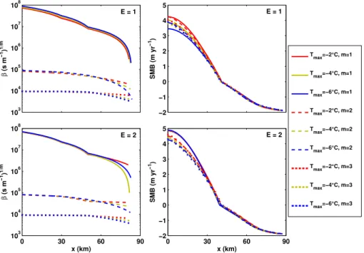
Fig. 1.Profiles of the (left) basal roughness factor,β, and (right) surface mass balance, SMB, for the 18 model simulations performed using the seaward-dipping bed profile. The basal roughness factor is plotted using a logarithmic scale to highlight the dependence of the chosen piecewise linear functions onm. The data are divided according to the enhancement factor,E, in order to highlight the differences between (top panels) normal,E=1, and (bottom panels) enhanced,E=2, ice deformation. Different colors distinguish the maximum ice
temperature (Tmax)used to calculate the rate factor profiles: red indicatesTmax= −2◦C, yellow indicatesTmax= −4◦C, and blue indicates
Tmax= −6◦C. The line style distinguishes the choice ofm: solid lines indicatem=1, dashed lines indicatem=2, and dotted lines indicate
m=3.
−2 −1 0 1 2 3 4 5
SMB (m yr
−1
)
E = 1
103
104
105
106
107
108
β
(s m
−1
)
1/m
E = 1
0 30 60 90 120
103
104
105
106
107
108
β
(s m
−1
)
1/m
x (km)
E = 2
0 30 60 90 120
−2 −1 0 1 2 3 4 5
SMB (m yr
−1
)
x (km)
E = 2
T
max=−2°C, m=1
T
max=−4°C, m=1
T
max=−6°C, m=1
T
max=−2°C, m=2
T
max=−4°C, m=2
T
max=−6°C, m=2
T
max=−2°C, m=3
T
max=−4°C, m=3
T
max=−6°C, m=3
−400 −200 0 200 400 600 h (m)
E = 1
2 4 6 8 10 12
U (m d
−1
)
E = 1
0.6 0.8 1 1.2 1.4 1.6
1.8x 10
−24
A (Pa
−3
s
−1) E = 1
50 60 70 80 90
−400 −200 0 200 400 600 h (m) x (km) E = 2
50 60 70 80 90
2 4 6 8 10 12
U (m d
−1)
x (km) E = 2
50 60 70 80 90
0.6 0.8 1 1.2 1.4 1.6
1.8x 10
−24
A (Pa
−3 s
−1
)
x (km) E = 2
T
max=−2°C, m=1
T
max=−4°C, m=1
T
max=−6°C, m=1
T
max=−2°C, m=2
T
max=−4°C, m=2
T
max=−6°C, m=2
T
max=−2°C, m=3
T
max=−4°C, m=3
T
max=−6°C, m=3
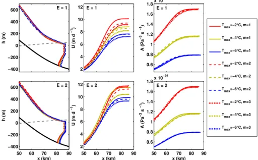
Fig. 3.Initial stable profiles of the (left panels) ice surface elevation, (center panels) speed, and (right panels) rate factor for the 18 model
simulations performed using the seaward-dipping bed profile.
−600 −400 −200 0 200 400 h (m)
E = 1
2 4 6 8
U (m d
−1
)
E = 1
0.4 0.6 0.8 1 1.2 1.4 1.6
1.8x 10
−24 A (Pa −3 s −1 )
E = 1
60 70 80 90 100 110
−600 −400 −200 0 200 400 h (m) x (km) E = 2
60 70 80 90 100 110
2 4 6 8
U (m d
−1)
x (km) E = 2
60 70 80 90 100 110
0.4 0.6 0.8 1 1.2 1.4 1.6
1.8x 10
−24
A (Pa
−3 s
−1
)
x (km) E = 2
T
max=−2°C, m=1
T
max=−4°C, m=1
T
max=−6°C, m=1
T
max=−2°C, m=2
Tmax=−4°C, m=2
T
max=−6°C, m=2
T
max=−2°C, m=3
T
max=−4°C, m=3
T
max=−6°C, m=3
Fig. 4.Initial stable profiles of the (left panels) ice surface elevation, (center panels) speed, and (right panels) rate factor for the 18 model simulations performed using the over-deepened bed profile.
the difference in ice thickness between the individual simu-lations and the ensemble mean (not shown) is within the up to 50 m-uncertainty of current ice thickness observations ac-quired from radio-echo sounding (Bamber et al., 2013). The calving front position varies by≤1 km relative to the
ensem-ble mean and flow speed at the ice front varies by less than 25 %, both of which fall within the range of observed sea-sonal variability in Greenland (Howat et al., 2010; Schild and
Hamilton, 2013). Thus, we consider all stable profiles to fall within the uncertainty range of the ensemble mean.
3.2 Transient simulations
−400 −200 0 200 400 600
h (m)
t=0yrs
2 6 10 14
U (m d
−1
)
t=0yrs
−400 −200 0 200 400 600
h (m)
t=1yr
2 6 10 14
U (m d
−1)
t=1yr
−400 −200 0 200 400 600
h (m)
t=5yrs
2 6 10 14
U (m d
−1
)
t=5yrs
−400 −200 0 200 400 600
h (m)
t=10yrs
2 6 10 14
U (m d
−1)
t=10yrs
50 60 70 80 90
−400 −200 0 200 400 600
h (m)
x (km)
t=20yrs
50 60 70 80 90
2 6 10 14
x (km)
U (m d
−1
)
t=20yrs
T
max=−2°C, m=1
T
max=−4°C, m=1
T
max=−6°C, m=1
T
max=−2°C, m=2
T
max=−4°C, m=2
T
max=−6°C, m=2
T
max=−2°C, m=3
T
max=−4°C, m=3
T
max=−6°C, m=3
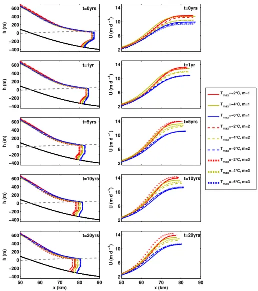
Fig. 5.Simulated profiles of (left panels) elevation and (right panels) speed at 0, 1, 5, 10, and 20 yr after the step increase in submarine melt rates for simulations performed using the seaward-dipping bed profile. Profiles are shown for the model simulations with enhanced ice deformation (i.e.,E=2).
magnitude of the dynamic response varies for each simula-tion as the result of differences in the bed geometry and the parameter values; therefore, to isolate the influence of param-eter uncertainty on the transient glacier response, the simu-lations performed using the different bed geometries are pre-sented separately.
3.2.1 Seaward-dipping bed profile simulations
The response of the simulated glaciers to the step increase in the submarine melt rate is strongly controlled by the value of the enhancement factor: doubling the enhancement factor fromE=1 toE=2 causes the change in grounding line
po-sition and discharge to approximately double following the onset of the perturbation. The pattern of retreat and acceler-ation following the onset of the step increase in submarine melting is the same for the E=1 andE=2 simulations,
−600 −400 −200 0 200 400
h (m)
t=0yrs
2 6 10 14
U (m d
−1
)
t=0yrs
−600 −400 −200 0 200 400
h (m)
t=1yr
2 6 10 14
U (m d
−1
)
t=1yr
−600 −400 −200 0 200 400
h (m)
t=5yrs
2 6 10 14
U (m d
−1
)
t=5yrs
−600 −400 −200 0 200 400
h (m)
t=10yrs
2 6 10 14
U (m d
−1)
t=10yrs
60 70 80 90 100 110
−600 −400 −200 0 200 400
h (m)
x (km)
t=20yrs
60 70 80 90 100 110
2 6 10 14
x (km)
U (m d
−1)
t=20yrs
T
max=−2°C, m=1
T
max=−4°C, m=1
T
max=−6°C, m=1
T
max=−2°C, m=2
T
max=−4°C, m=2
T
max=−6°C, m=2
T
max=−2°C, m=3
T
max=−4°C, m=3
T
max=−6°C, m=3
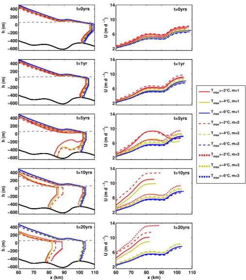
Fig. 6.Simulated profiles of (left panels) elevation and (right panels) speed at 0, 1, 5, 10, and 20 yr after the step increase in submarine
melt rates for simulations performed using the over-deepened bed profile. Profiles are shown for the model simulations with enhanced ice deformation (i.e.,E=2).
intra-annual variations in the extent and discharge of each simulated glacier shown in Fig. 7 are due to the use of dis-crete time steps in the model simulations, which cause the grounding line position to fluctuate by 10s of meters. These variations do not influence the overall response of the glacier to the perturbation.
3.2.2 Over-deepened bed profile simulations
In the absence of enhanced ice deformation (i.e.,E=1), the
simulated glaciers remain grounded seaward of the basal de-pression despite measurable thinning and acceleration within the outlet channel (not shown). Thinning and acceleration cause the grounding line to retreat 1.5–2.4 km into shallower water towards the crest of the shoal. Similar to the E=1
simulations performed using the seaward-dipping bed
pro-file, the grounding line discharge initially increases by 1.5– 5 %, then slowly decreases towards pre-perturbed values.
For the simulations with enhanced ice deformation (i.e., E=2), the transient response to the increase in the
subma-rine melt rate is bimodal: the glaciers either initially thin and accelerate but remain grounded on the shoal and ap-proach a new stable configuration, or the initial thinning and acceleration bring the ice to flotation in the basal depres-sion, triggering much larger retreat, acceleration, and thin-ning (Fig. 6). The magnitude of grounding line retreat and increase in discharge vary by a factor of∼1.5 (1.7–2.7 km)
and 5 (0.8–4 %), respectively, for the glaciers that remain grounded across the basal depression (Fig. 8). In contrast, for the four glaciers that unstably retreat∼22 km across the
−10 −8 −6 −4 −2 0
dx
front
(km)
−10 −8 −6 −4 −2 0
dx
gl
(km)
0 2 4 6 8 10 12 14 16 18 20
0 0.05 0.1 0.15 0.2
Time (yrs)
dQ
gl
T
max=−2°C, m=1
T
max=−4°C, m=1
T
max=−6°C, m=1
T
max=−2°C, m=2
T
max=−4°C, m=2
T
max=−6°C, m=2
T
max=−2°C, m=3
T
max=−4°C, m=3
T
max=−6°C, m=3
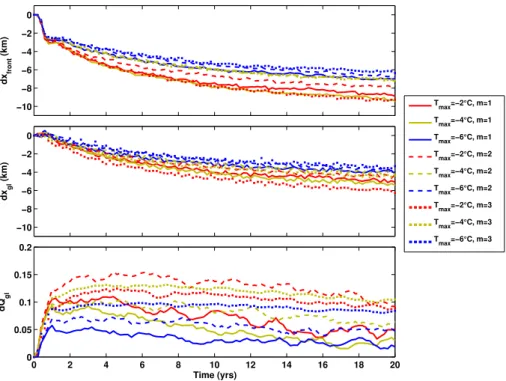
Fig. 7.Time series of (top panel) front position change, (middle panel) grounding line change, and (bottom panel) the fractional increase
in grounding line discharge relative to the initial discharge for simulations performed using the seaward-dipping bed profile. As in Fig. 5, profiles are shown for the model simulations with enhanced ice deformation (i.e.,E=2).
4 Discussion
The results of our model simulations suggest that a non-unique combination of parameter values can produce simi-lar stable glacier configurations, as previously demonstrated by Arthern and Gudmundsson (2010). If the accumulation rate uncertainty is restricted to 5 %, the range of parameter combinations used in the model simulations can be reduced to 8 of the 18 parameter combinations. Although the culling procedure is likely to eliminate incorrect parameter combina-tions, the dynamic response of the culled simulations varies with the choice of parameter values used to describe the ice rheology and basal sliding.
We find that dynamic thinning rates within the outlet chan-nel vary with the rate factor or enhancement factor of the simulated glacier, leading to differences in grounding line retreat following the onset of the step perturbation. The rate of dynamic thinning increases as the rate and enhance-ment factors increase, such that the magnitude of ground-ing line retreat is larger for glaciers with higher ice tem-peratures (Figs. 7, 8; temtem-peratures distinguished by color) or enhanced deformation. As demonstrated by the simula-tions performed using the over-deepened bed profile, differ-ences in the ice flow from±2◦C uncertainty in the
maxi-mum ice temperature can strongly influence the dynamic re-sponse of glaciers that are initially close to flotation across reverse bed slopes because a small perturbation can bring the ice to flotation (i.e., thickness threshold), triggering a much
larger response (Figs. 6, 8). For the simulations obtained with a linear basal sliding relation and enhanced ice deformation (Figs. 6, 8; solid lines), dynamic thinning brings the two sim-ulated glaciers with higher ice temperatures (Tmax= −2◦C
and−4◦C) to flotation within the depression<5 yr after the onset of the perturbation, triggering the rapid and unstable re-treat of the grounding line. In contrast, the simulated glacier with the lowest ice temperature profile (Tmax= −6◦C)
re-mains grounded on the shoal throughout the 20 yr transient simulation (Figs. 6, 8; solid blue lines). Given that the respec-tive differences in the initial ice thickness (<30 m) and speed (<0.1 m d−1)for the Tmax= −4◦C andTmax= −6◦C
sim-ulations are within the typical observational uncertainty for real glacier systems, either combination of parameter values could be used to simulate the initial stable glacier configura-tion in the absence of precise temperature measurements.
−25 −20 −15 −10 −5 0
dx
front
(km)
−25 −15 −5
dx
gl
(km)
0 2 4 6 8 10 12 14 16 18 20
0 0.1 0.2 0.3 0.4 0.5
Time (yrs)
dQ
gl
T
max=−2°C, m=1
T
max=−4°C, m=1
T
max=−6°C, m=1
T
max=−2°C, m=2
T
max=−4°C, m=2
T
max=−6°C, m=2
T
max=−2°C, m=3
T
max=−4°C, m=3
T
max=−6°C, m=3
Fig. 8.Time series of (top panel) front position change, (middle panel) grounding line change, and (bottom panel) the fractional increase in
grounding line discharge relative to the initial discharge for simulations performed using the over-deepened bed profile. As in Fig. 6, profiles are shown for the model simulations with enhanced ice deformation (i.e.,E=2).
The influence of the basal sliding exponent on the transient glacier behavior is clearly shown in the discharge time series for theE=2 andTmax= −2◦C simulations performed using
the over-deepened bed geometry (Fig. 8; red lines). Further, the choice of the basal roughness parameter influences both the timing and magnitude of retreat, such that the response of the simulated glaciers does not necessarily vary systemat-ically with the ice rheology, as demonstrated by differences in the grounding line retreat time series in Figs. 7 and 8.
5 Implications for modeling of real glacier systems
Although our simulations were performed using a depth-integrated flowline model for analytical simplicity and com-putational efficiency, the ice rheology and basal sliding pa-rameterizations we test are inherent in all numerical ice flow models. Therefore, our results suggest that in some cases, prognostic ice flow models cannot be used to confidently pre-dict the precise timing and magnitude of changes in glacier behavior due to uncertainty in the ice rheology and basal slid-ing parameterizations. Confidence in prognostic models can be improved, however, by comparing the modeled transient behavior with precise measurements of the initial and tran-sient glacier configurations (i.e., hindcasting, Aschwanden et al., 2013). Using a hindcasting approach, simulations that fail to reproduce the observed temporal evolution of the glacier are rejected, restricting the range of parameters used in
prog-nostic simulations. The benefit of hindcasting is clearly illus-trated in Fig. 8: if similar transient results were obtained for a real glacier system with annual front position and speed time series, these data could be used to assess the validity of the different model simulations, which would likely improve the accuracy of prognostic simulations.
Of particular importance is that small differences in the rheology of the ice from temperature uncertainty of±2◦C
can determine whether or not a glacier initially grounded across a basal depression will reach the threshold for un-stable retreat. The high sensitivity of predicted behavior to differences in ice rheology has two major implications for modeling of real glacier systems. First, given that the uncer-tainty in the width- and depth-integrated ice temperature for real glacier systems is probably much larger than the±2◦C
the model’s ability to simulate the period of rapid grounding line retreat and acceleration. The model, however, was un-able to reproduce the continued acceleration of the glacier as the rate of grounding line retreat decreased (Vieli and Nick, 2011), potentially indicating that the aforementioned feed-back between acceleration and shear softening could not be accounted for using a constant enhancement factor. Thus, for real glacier systems, it is likely that temporal changes in the ice rheology and basal sliding parameterizations must also be accounted for in order to accurately simulate temporal changes in glacier behavior.
In order to improve confidence in predictions of glacier be-havior, we suggest that the initial ice rheology is constrained by temperature and surface strain rate measurements that can be used to calculate the effective viscosity of the ice. Further, if available, past changes in dynamics should be used to con-strain the basal sliding exponent and temporal changes in the ice rheology due to strain heating and damage. To restrict the choice of appropriate parameter values, model simula-tions should be performed using a range of parameter values and simulations that successfully reproduce the initial and transient glacier thickness and speed profiles, as well as the position of the calving front. Simulations that successfully reproduce past glacier configurations can then be used to pre-dict the most likely range of glacier behavior in response to changes in external forcing.
6 Conclusions
In order to investigate the sensitivity of prognostic flowline models to uncertainty in ice rheology and basal sliding pa-rameterizations, we vary the rate factor, enhancement factor, and basal sliding exponent across 18 simulations performed using a previously published flowline model. We find that al-though a non-unique combination of parameter values can be used to produce similar initial stable configurations, differ-ences in the ice rheology, from uncertainty in the rate factor (through temperature) or the enhancement factor, strongly in-fluence the magnitude of grounding line retreat in response to external forcing. Similarly, differences in the basal sliding exponent control the magnitude of glacier acceleration re-quired to restore grounding line stability following the onset of retreat, with larger basal sliding exponents corresponding to larger fractional changes in ice flow speed. Precise mea-surements of the initial and transient glacier configurations can be used to restrict the range of parameter values used in the model simulations through hindcasting, however, a non-unique combination of ice rheology and basal sliding param-eterizations may still exist. Based on these results, as well as the high sensitivity of flowline models to uncertainty in geometry parameterizations (Enderlin et al., 2013), we con-clude that in order to confidently predict glacier behavior, flowline models applied to real glacier systems must be ac-companied by sensitivity tests that take into account the
un-certainty in model parameters. In the absence of such sensi-tivity tests, we suggest that the use of prognostic flowline models is restricted to the prediction of long-term trends rather than to precisely constraining the timing of future changes in dynamics.
Acknowledgements. We would like to thank Olivier Gagliardini,
Andy Aschwanden, and an anonymous reviewer for their useful comments. This work was funded by a NASA Earth and Space Science Fellowship to E. M. Enderlin.
Edited by: O. Gagliardini
References
Applegate, P. J., Kirchner, N., Stone, E. J., Keller, K., and Greve, R.: An assessment of key model parametric uncertainties in projec-tions of Greenland Ice Sheet behavior, The Cryosphere, 6, 589– 606, doi:10.5194/tc-6-589-2012, 2012.
Arthern, R. J. and Gudmundsson, G. H.: Initialization of ice-sheet forecasts viewed as an inverse Robin problem, J. Glaciol., 56, 197, 527–533, 2010.
Aschwanden, A., Aðalgeirsdóttir, G., and Khroulev, C.: Hindcast-ing to measure ice sheet model sensitivity to initial states, The Cryosphere, 7, 1083–1093, doi:10.5194/tc-7-1083-2013, 2013. Bamber, J. L., Griggs, J. A., Hurkmans, R. T. W. L., Dowdeswell,
J. A., Gogineni, S. P., Howat, I., Mouginot, J., Paden, J., Palmer, S., Rignot, E., and Steinhage, D.: A new bed elevation dataset for Greenland, The Cryosphere, 7, 499–510, doi:10.5194/tc-7-499-2013, 2013.
Bartholomew, I., Nienow, P., Mair, D., Hubbard, A. King, M., and Sole, A.: Seasonal evolution of subglacial drainage and accel-eration in a Greenland outlet glacier, Nat. Geosci., 3, 408–411, doi:10.1038/NGEO863, 2010.
Benn, D. I., Warren, C. R., and Mottram, R. H.: Calving processes and the dynamics of calving glaciers, Earth-Sci. Rev., 82, 143– 179, 2007.
Burgess, E. W., Forster, R. R., Box, J. E., Mosley-Thompson, E., Bromwich, D. H., Bales, R. C., and Smith, L. C.: A spatially calibrated model of annual accumulation rate on the Green-land Ice Sheet (1958–2007), J. Geophys. Res., 115, F02004, doi:10.1029/2009JF001293, 2010.
Colgan, W., Pfeffer, W. T., Rajaram, H., Abdalati, W., and Balog, J.: Monte Carlo ice flow modeling projects a new stable config-uration for Columbia Glacier, Alaska, c. 2020, The Cryosphere, 6, 1395–1409, doi:10.5194/tc-6-1395-2012, 2012.
Cornford, S. L., Martin, D. F., Graves, D. T., Ranken, D. F., Le Brocq, A. M., Gladstone, R. M., Payne, A. J., Ng, E. G., and Lip-scomb, W. H.: Adaptive mesh, finite volume modeling of marine ice sheets, J. Comp. Phys., 232, 529–549, 2013.
Cuffey, K. M. and Paterson, W. S. B.: The Physics of Glaciers, 4th Edn., Elsevier, Amsterdam, 2010.
Enderlin, E. M. and Howat, I. M.: Submarine melt rate estimates for floating termini of Greenland outlet glaciers (2000–2010), J. Glaciol., 59, 67–75, doi:10.3189/2013JoG12J049, 2013. Enderlin, E. M., Howat, I. M., and Vieli, A.: High sensitivity of
Ettema, J., van den Broeke, M. R., van Meijgaard, E., van de Berg, W. J., Bamber, J. L., Box, J. E., and Bales, R. C.: Higher sur-face mass balance of the Greenland ice sheet revealed by high-resolution climate modeling, Geophys. Res. Lett., 36, L12501, doi:10.1029/2009GL038110, 2009.
Favier, L., Gagliardini, O., Durand, G., and Zwinger, T.: A three-dimensional full Stokes model of the grounding line dynamics: effect of a pinning point beneath the ice shelf, The Cryosphere, 6, 101–112, doi:10.5194/tc-6-101-2012, 2012.
Gagliardini, O., Durand, G., Zwinger, T., Hindmarsh, R. C. A., and Le Meur, E.: Coupling of ice shelf melting and buttressing is a key process in ice sheets dynamics, Geophys. Res. Lett., 37, L14501, doi:10.1029/2010GL043334, 2010.
Gladstone, R. M., Lee, V., Rougier, J., Payne, A. J., Hellmer, H., Le Brocq, A., Shepherd, A., Edwards, T. L., Gregory, J., and Cornford, S. L.: Calibrated prediction of Pine Island Glacier re-treat during the 21st and 22nd centuries with a coupled flowline model, Earth Planet. Sc. Lett., 333, 191–199, 2012.
Greve R., Saito, F., and Abe-Ouchi, A.: Initial results of the SeaRISE numerical experiments with the models SICOPOLIS and IcIES for the Greenland Ice Sheet, Ann. Glaciol., 52, 23–30, 2011.
Gudmundsson, G. H.: Basal-flow characteristics of a non-linear flow sliding frictionless over strongly undulating bedrock, J. Glaciol., 43, 143, 80–89, 1997.
Gudmundsson, G. H., Krug, J., Durand, G., Favier, L., and Gagliar-dini, O.: The stability of grounding lines on retrograde slopes, The Cryosphere, 6, 1497–1505, doi:10.5194/tc-6-1497-2012, 2012.
Howat, I. M., Box, J. E., Ahn, Y., Herrington, A., and McFadden, E. M.: Seasonal variability in the dynamics of marine-terminating outlet glaciers in Greenland, J. Glaciol., 56, 198, 601–613, 2010. Hulbe, C. L., Scambos, T. A., Youngberg, T., and Lamb, A. K.: Patterns of glacier response to disintegration of the Larsen B ice shelf, Antarctic Peninsula, Global Planet. Change, 63, 1–8, doi:10.1016/j.gloplacha.2008.01.001, 2008.
Jamieson, S. S. R., Vieli, A., Livingstone, S. J., Ó Cofaigh, C., Stokes, C., Hillenbrand, C.-D., and Dowdeswell, J. A.: Ice-stream stability on a reverse bed slope, Nat. Geosci., 5, 799–802, doi:10.1038/NGEO1600, 2012.
Joughin, I., Smith, B. E., Howat, I. M., Scambos, T., and Moon, T.: Greenland flow variability from ice-sheet-wide velocity map-ping, J. Glaciol., 56, 415–430, 2010.
Morlighem, M., Rignot, E., Seroussi, H., Larour, E., Ben Dhia, H., and Aubry, D.: Spatial patterns of basal drag inferred using con-trol methods from a full-Stokes and simpler models for Pine Is-land Glacier, West Antarctica, Geophys. Res. Lett., 37, L14502, doi:10.1029/2010GL043853, 2010.
Nick, F. M., van der Kwast, J., and Oerlemans, J.: Simulation of the evolution of Breidamerkurjökull in the late Holocene, J. Geo-phys. Res., 112, B01103, doi:10.1029/2006JB004358, 2007a. Nick, F. M., van der Veen, C. J., and Oerlemans, J.: Controls on
advance of tidewater glaciers: Results from numerical model-ing applied to Columbia Glacier, J. Geophys. Res., 112, F03S24, doi:10.1029/2006JF000551, 2007b.
Nick, F. M., Vieli, A., Howat, I., and Joughin, I.: Large-scale changes in Greenland outlet glacier dynamics triggered at the ter-minus, Nat. Geosci., 2, 110–114, doi:10.1038/NGEO394, 2009. Nick, F. M., van der Veen, C. J., Vieli, A., and Benn, D. I.: A phys-ically based calving model applied to marine outlet glaciers and implications for their dynamics, J. Glaciol., 56, 199, 781–794, 2010.
Nick, F. M., Luckman, A., Vieli, A., van der Veen, C. J., van As, D., van de Wal, R. S. W., Pattyn, F., Hubbard, A., and Floricioiu, D.: The response of Petermann Glacier, Greenland, to large calving events, and its future stability in the context of atmospheric and oceanic warming, J. Glaciol., 58, 229–239, doi:10.3189/2012JoG11J242, 2012.
Nick, F. M., Vieli, A., Anderson, M. L., Joughin, I., Payne, A., Ed-wards, T. L., Pattyn, F., and van de Wal, R. S. W.: Future sea-level rise from Greenland’s main outlet glaciers in a warming climate, Nature, 497, 235–238, doi:10.1038/nature12068, 2013. Pattyn, F., Schoof, C., Perichon, L., Hindmarsh, R. C. A., Bueler,
E., de Fleurian, B., Durand, G., Gagliardini, O., Gladstone, R., Goldberg, D., Gudmundsson, G. H., Huybrechts, P., Lee, V., Nick, F. M., Payne, A. J., Pollard, D., Rybak, O., Saito, F., and Vieli, A.: Results of the Marine Ice Sheet Model Intercomparison Project, MISMIP, The Cryosphere, 6, 573–588, doi:10.5194/tc-6-573-2012, 2012.
Pfeffer, W. T.: A simple mechanism for irreversible tide-water glacier retreat, J. Geophys. Res., 112, F03S25, doi:10.1029/2006JF000590, 2007.
Rignot, E.: Changes in West Antarctic ice stream dynamics ob-served with ALOS PALSAR data, Geophys. Res. Lett., 35, L12505, doi:10.1029/2008GL033365, 2008.
Rignot, E. and Steffen, K.: Channelized bottom melting and stabil-ity of floating ice shelves, Geophys. Res. Lett., 35, 2, L02503, doi:10.1029/2007GL031765, 2008.
Schild, K. M. and Hamilton, G. S.: Seasonal variations of outlet glacier terminus position in Greenland, J. Glaciol., 59, 759–770, doi:10.3189/2013JoG12J238, 2013.
Schoof, C.: The effect of cavitation on glacier sliding, P. Roy. Soc. A-Math. Phy., 461, 609–627, doi:10.1098/rspa.2004.1350, 2005. Schoof, C.: Ice sheet grounding line dynamics: Steady-states, stability and hysteresis, J. Geophys. Res., 112, F03S28, doi:10.1029/2006JF000664, 2007.
Stone, E. J., Lunt, D. J., Rutt, I. C., and Hanna, E.: Investigating the sensitivity of numerical model simulations of the modern state of the Greenland ice-sheet and its future response to climate change, The Cryosphere, 4, 397–417, doi:10.5194/tc-4-397-2010, 2010. Vieli, A. and Nick, F. M.: Understanding and modeling rapid
dy-namic changes of tidewater outlet glaciers: Issues and impli-cations, Surv. Geophys., 32, 437–458, doi:10.1007/s10712-011-9132-4, 2011.