Temperature response functions introduce high uncertainty in modelled carbon stocks in cold temperature regimes

(1)

BGD

6, 8129–8165, 2009

Temperature response functions

and their uncertainties

H. Portner et al.

Title Page

Abstract Introduction

Conclusions References

Tables Figures

◭ ◮

Back Close

Full Screen / Esc

Printer-friendly Version

Interactive Discussion Biogeosciences Discuss., 6, 8129–8165, 2009

www.biogeosciences-discuss.net/6/8129/2009/ © Author(s) 2009. This work is distributed under the Creative Commons Attribution 3.0 License.

Biogeosciences Discussions

Biogeosciences Discussionsis the access reviewed discussion forum ofBiogeosciences

Temperature response functions

introduce high uncertainty in modelled

carbon stocks in cold temperature

regimes

H. Portner, H. Bugmann, and A. Wolf

Forest Ecology, Institute of Terrestrial Ecosystems, Department of Environmental Sciences, ETH Z ¨urich, 8092 Z ¨urich, Switzerland

Received: 8 July 2009 – Accepted: 3 August 2009 – Published: 12 August 2009

Correspondence to: H. Portner (hanspeter.portner@env.ethz.ch)

(2)

BGD

6, 8129–8165, 2009

H. Portner et al.

Title Page

Tables Figures

◭ ◮

Back Close

Full Screen / Esc

Interactive Discussion

Abstract

Models of carbon cycling in terrestrial ecosystems contain formulations for the depen-dence of respiration on temperature, but the sensitivity of predicted carbon pools and fluxes to these formulations and their parameterization is not understood. Thus, we made an uncertainty analysis of soil organic matter decomposition with respect to its

5

temperature dependency using the ecosystem model LPJ-GUESS.

We used five temperature response functions (Exponential, Arrhenius, Lloyd-Taylor, Gaussian, Van’t Ho_ff). We determined the parameter uncertainty ranges of the func-tions by nonlinear regression analysis based on eight experimental datasets from northern hemisphere ecosystems. We sampled over the uncertainty bounds of the

10

parameters and run simulations for each pair of temperature response function and calibration site. The uncertainty in both long-term and short-term soil carbon dynamics was analyzed over an elevation gradient in southern Switzerland.

The function of Lloyd-Taylor turned out to be adequate for modelling the temperature dependency of soil organic matter decomposition, whereas the other functions either

15

resulted in poor fits (Exponential, Arrhenius) or were not applicable for all datasets (Gaussian, Van’t Ho_ff). There were two main sources of uncertainty for model simula-tions: (1) the uncertainty in the parameter estimates of the response functions, which increased with increasing temperature and (2) the uncertainty in the simulated size of carbon pools, which increased with elevation, as slower turn-over times lead to higher

20

carbon stocks and higher associated uncertainties. The higher uncertainty in carbon pools with slow turn-over rates has important implications for the uncertainty in the pro-jection of the change of soil carbon stocks driven by climate change, which turned out to be more uncertain for higher elevations and hence higher latitudes, which are of key importance for the global terrestrial carbon budget.

(3)

BGD

6, 8129–8165, 2009

H. Portner et al.

Title Page

Tables Figures

◭ ◮

Back Close

Full Screen / Esc

1 Introduction

Anthropogenic CO₂emissions from fossil fuel consumption, cement-manufacturing and deforestation are leading to an increase in atmospheric CO₂concentrations, thus inducing considerable changes of the climate at global, regional and local scales (Solomon et al., 2007). Atmospheric CO₂concentrations are also strongly a_ffected by

5

changes in the major global natural carbon reservoirs. For example, at present signif-icantly more carbon is stored in the world’s soils than in the atmosphere (Schlesinger, 1997). Climatic changes have a direct impact on global soil carbon stocks, but their quantification is subject to considerable debate and disagreement (Davidson and Janssens, 2006; Kirschbaum, 2006; Hakkenberg et al., 2008). If significant amounts

10

of carbon currently stored as organic matter belowground are transferred to the atmo-sphere by a warming-induced acceleration of decomposition, a positive feedback to climate change may occur (Bronson et al., 2008). Conversely, if increases of plant-derived carbon inputs to soils exceed increases in decomposition, the feedback would be negative. Despite much research, a consensus has not yet emerged on the climate

15

sensitivity of soil carbon decomposition.

Soil respiration is commonly divided into two components: root respiration with asso-ciated mycorrhizal respiration and soil organic matter (SOM) decomposition. We focus on SOM decomposition here. SOM has turnover times ranging from years to decades and even centuries. It is often conceptualised as several distinct pools with

increas-20

ing residence times (Knorr et al., 2005; Kirschbaum, 2004; Eliasson et al., 2005) or as continuous with gradual decay rates ( ˚Agren and Bosatta, 1987; Bosatta and ˚Agren, 1999). Decomposition of SOM is highly complex, as it is driven by a combination of fac-tors such as temperature (Berg and Laskowski, 2005a), moisture conditions (Cisneros-Dozal et al., 2006) and its chemical quality (Berg and Laskowski, 2005b; Weedon et al.,

25

2009; Cornwell et al., 2008).

(4)

BGD

6, 8129–8165, 2009

H. Portner et al.

Title Page

Tables Figures

◭ ◮

Back Close

Full Screen / Esc

Interactive Discussion process of carbon uptake (photosynthesis) is represented in a fairly detailed manner

in these models, the equally important process of carbon release by soil respiration is represented in a comparatively simple manner (Cramer et al., 2001; Friedlingstein et al., 2006). Among others, there is no agreement on the choice of the form of the response function that is used to describe the sensitivity of soil carbon decomposition

5

to temperature.

We focus on the sensitivity of a widely used biosphere model, LPJ-GUESS (Smith et al., 2001), to a range of possible formulations for the temperature dependency of soil organic matter decomposition, in order to evaluate their assets and drawbacks.

We assess the impact of uncertainty in the formulation of the temperature response

10

of heterotrophic respiration on estimates of present and future carbon storage in ecosystems and hence on the CO₂feedback to the atmosphere. We specifically inves-tigate the relative importance of the model formulation vs. the uncertainty introduced by using di_fferent parameterization data sets. We quantify the resulting impacts with re-gard to both short-term carbon fluxes and long-term carbon storage along an elevation

15

gradient in southern Switzerland.

2 Methods

We chose a holistic approach and considered not only the raw fits of candidate func-tions to calibration datasets, but also the number of parameters, the uncertainty in parameter estimates and the uncertainty in model output variables. We placed a

spe-20

cial focus on the identification of a suitable model formulation that not only fitted well to experimental data, but also led to acceptable uncertainty in the output variables when employed in LPJ-GUESS.

In biogeochemical models, the relationship between SOM decomposition and soil temperature is often described by one out of a set of related functions. We tested five

25

(5)

BGD

6, 8129–8165, 2009

H. Portner et al.

Title Page

Tables Figures

◭ ◮

Back Close

Full Screen / Esc

Interactive Discussion The Exponential and Arrhenius functions are simplifications of the function proposed

by Van’t Ho_ff(1901). Lloyd and Taylor (1994) proposed a modified Arrhenius function and Tuomi et al. (2008); O’Connell (1990) a Gaussian function. The details of the five functions are described below.

We built upon the well-established LPJ-GUESS model (Smith et al., 2001) and soil

5

respiration data from di_fferent Ameriflux and CarboEuropeIP sites (Hibbard et al., 2005, 2006). We used only one ecosystem model to avoid further uncertainties introduced by di_fferent representations of other processes which typically arise in model inter-comparisons (Cramer et al., 2001; Morales et al., 2005). The Ticino catchment in southern Switzerland with its large climate gradient was used as a case study to

evalu-10

ate the sensitivity of the model to the uncertainty in model parameters with respect to di_fferent process formulations and calibration datasets with varying temperature regimes.

2.1 The LPJ-GUESS model

We used the dynamic ecosystem model LPJ-GUESS (Smith et al., 2001; Sitch et al.,

15

2003). The model framework incorporates process-based representations of plant physiology, establishment, competition, mortality and ecosystem biogeochemistry. LPJ-GUESS has been successful in predicting vegetation distribution, net primary pro-duction and net ecosystem exchange in many di_fferent ecosystems (Smith et al., 2001; Morales et al., 2007).

20

2.1.1 LPJ-GUESS soil module

Soil carbon in LPJ-GUESS is divided into three distinct pools: litter, slow SOM and fast SOM. The temporal dynamics of the carbon stock (C_i) of each individual pool (i) are modeled on a daily basis; they follow first-order kinetics with a decay rate k_i (Eq. 1). The decay rate itself depends on soil temperature and soil moisture, expressed as the

25

product of the decay ratek_{i ,T}

(6)

BGD

6, 8129–8165, 2009

H. Portner et al.

Title Page

Tables Figures

◭ ◮

Back Close

Full Screen / Esc

Interactive Discussion response functionR_T and the moisture response functionR_M (Eq. 2). The decay rate

k_{i ,T}

ref is the reciprocal of turnover timeτi ,Tref.

∆C_i

∆t =−ki×Ci (1)

k_i ₌k_{i ,T}

ref ×RT ×RM (2)

Litter from leaves, roots and tree stems is added to the litter pool at the end of each

5

simulation year. Each of the three carbon pools has its own specific turnover time (τ_{i ,T}

ref) at reference temperature Tref=10

◦_{C and ample soil moisture: 2.85 y, 33 y and}

1000 y, respectively (Meentemeyer, 1978; Foley, 1995). The mineralized litter is di-vided into three parts, 70% are respired, whereas 0.45% are transferred to the slow and 29.55% to the fast SOM pool (Foley, 1995). Both SOM pools then undergo

de-10

composition independently, i.e. without feedbacks to the other pools.

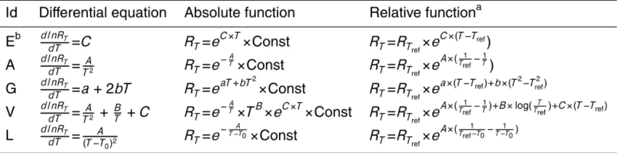
2.1.2 Temperature response functions implemented in LPJ-GUESS

Five potential response functions were implemented in the model (Table 1). The Ex-ponential response function (E) features a constantQ₁₀ value. It is motivated by Van’t Hoffs rule, stating that the rate of a reaction increases two- to threefold for an increase

15

in temperature by 10◦_{C (Van’t Ho}

ff, 1901). The Arrhenius function (A) is based on the concept of an activation energy for chemical and biological reactions. However, realiz-ing that the change of the rate is not constant over temperatures, Van’t Hofftherefore suggested a more complex formula (V). Importantly, the Exponential and Arrhenius formulations are direct derivatives of the Van’t Hoffformulation, obtained by setting the

20

parametersA₌B₌0 andC₌B₌0, respectively. The response function in the standard implementation of LPJ-GUESS is based on Lloyd and Taylor (1994) (L). It is a variant of the Arrhenius function, suggested by Lloyd and Taylor (1994), because it often leads to better fits against empirical data by allowing for a decrease in activation energy with increasing energy. It must meet the condition T >T₀. The Gaussian function (G) in

(7)

BGD

6, 8129–8165, 2009

H. Portner et al.

Title Page

Tables Figures

◭ ◮

Back Close

Full Screen / Esc

Interactive Discussion turn is based on Lloyd-Taylor, by taking into account the first three terms of the

Tay-lor series expansion of the exponent of the Lloyd-TayTay-lor function (Tuomi et al., 2008; O’Connell, 1990). Note that the Exponential, Arrhenius and Lloyd-Taylor functions are monotonically rising functions, whereas the Gaussian and the Van’t Hofffunctions have a maximum.

5

As the decay constant k_{i ,T}

ref is valid only at the reference temperature Tref, the

re-sponse functions were expressed relative to this temperature (Table 1). We thus repa-rameterized the functions by combining Eqs. (3–4), leading to the general scheme of Eq. (5), wheref_abs,f_relandR_T

ref refer to the absolute and the relative response functions

and to the reference respiration at a given reference temperatureT_ref, respectively.

10

R_T ₌f_abs(T)_×Const (3)

R_T

ref =fabs(Tref)×Const (4)

R_T ₌R_T

ref ×frel(T , Tref) (5)

In the default version of LPJ-GUESS, autotrophic (root and mycorrhiza) and het-erotrophic soil respiration (SOM decomposition) are modelled using the same

re-15

sponse function. As we focused on decomposition here, the heterotrophic soil respira-tion was varied using the five alternative formularespira-tions introduced above, but autotrophic soil respiration was modeled based on the standard response function of Lloyd-Taylor in all simulations shown below.

2.2 Fitting of the temperature response functions

20

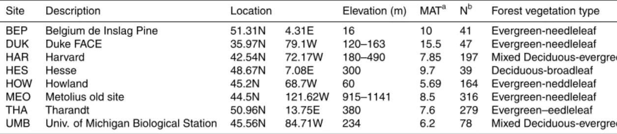
We used the database compiled by Hibbard et al. (2006), which contains datasets of soil respiration from different experimental sites of the northern hemisphere in Eu-rope and America. Eight sites were selected for calibration (Table 2) to reflect forest vegetation types that are significant for our research area (evergreen-needleleaf, mixed deciduous-evergreen, deciduous-broadleaf); we only used datasets that provided more

(8)

BGD

6, 8129–8165, 2009

H. Portner et al.

Title Page

Tables Figures

◭ ◮

Back Close

Full Screen / Esc

Interactive Discussion than 30 measurements of temperature and soil respiration. Measurements were made

on a daily basis, distributed over the whole year for time periods ranging from 1995 to 2002, depending on the site.

In nonlinear regression, the usual parameter confidence intervals cannot be used be-cause the parameters show non-linear behavior. Therefore, we first linearized all five

5

standardized functions using the method of expected-value parameters (Ratkowsky, 1990). We linearized for all but the parameterR_T

ref. The parameters of the

reparam-eterized functions exhibited close-to-linear behavior and therefore were characterized by almost exact confidence intervals (Appendix Table A1). The resulting functions were normalized (R_T

norm) to 1 by dividing by the best fit parameter estimate of the reference 10

respirationR_T

ref (Eq. 6).

R_T

norm=(RTref)

−1

×RT (6)

We used all five response functions at all eight sites and performed nonlinear fits for each dataset-function pair using nonlinear least-squares estimates in the statistics software packageR (R Development Core Team, 2008).

15

To fit the Van’t Ho_ff function, we introduced an additional data point in each data set at (−40◦C , 0µmol C m−2s1) to ensure that the function converges to zero when approaching the absolute zero temperature (0 K). We determined the 99% confidence intervals for each parameter of each function and the correlation matrix of the param-eters for each individual fit. The goodness of each fit was quantified by the Bayesian

20

information criterion (BIC) introduced by Schwarz (1978).

Using the 99% confidence intervals of the parameters, we created a sample of pa-rameter sets over their corresponding confidence range for each response function-site pair. We further discriminated between two cases: In the case woτ (without τ), we sampled over the confidence intervals of the response function parameters only. In the

25

(9)

BGD

6, 8129–8165, 2009

H. Portner et al.

Title Page

Tables Figures

◭ ◮

Back Close

Full Screen / Esc

Interactive Discussion respectively, as suggested by Parton et al. (1987). We thus assumed implicitly that

the turnover times neither depended on each other nor on the other parameters of the response functions.

We used the SIMLAB software from the European Joint Research Center (Saltelli et al., 2004) to generate the parameter sample sets. For each fit, we generated a latin

5

hypercube sample (N₌20). We sampled uniformly over the confidence intervals of the parameters and included the parameter dependences through the correlation matrix obtained in the fitting procedure based on the method of Iman and Conover (1982).

2.3 Simulations with LPJ-GUESS

2.3.1 Interpolation of climate data

10

LPJ-GUESS is driven by daily weather input, including mean temperature, precipita-tion sum, percentage sun-shine and atmospheric CO₂concentration. The climate data were compiled for an elevation transect in the Ticino catchment in the Southern Swiss Alps ranging from 300 to 2300 m a.s.l., sampled at 200 m intervals, resulting in a total of 11 individual sites.

15

Climate data for the period of 1901–2006 were compiled from different sources. Daily mean temperatures and daily precipitation sums for the period of 1960–2006 were ob-tained from a spatially explicit climate data set of whole Switzerland with a spatial resolution of 1 ha. The data were derived using the DAYMET model (Thornton et al., 1997), which was developed specifically for complex terrain such as mountain ranges

20

(data source: Land Use Dynamics, Swiss Federal Institute for Forest, Snow and Land-scape Research, Switzerland). Each elevation level was calculated as the mean of 100 adjacent grid points (10×10) taken from a south-facing slope.

Temperature and precipitation data for the period of 1935–1959 were based on the nearest automated meteorological station Locarno-Monti (distance 24 km), which

25

(10)

BGD

6, 8129–8165, 2009

H. Portner et al.

Title Page

Tables Figures

◭ ◮

Back Close

Full Screen / Esc

Interactive Discussion Unit (CRU TS 1.2, Mitchell et al., 2003). The anomalies of randomly selected years of

the reference station were applied to the monthly values of the CRU TS 1.2 dataset to obtain a set of daily values. The final datasets for all 11 elevation levels were based on this reference dataset, by shifting it to the actual mean and rescaling it to the observed range at each specific elevation level.

5

The dataset for percentage sunshine was based on the reference station Locarno-Monti (1960–2006) and the CRU TS 1.2 dataset for the period of 1901–1959. The same dataset was used for all elevation levels.

For the future, i.e. from 2007 to 2106, we chose the SRES A2 scenario data from the PRUDENCE project (Christensen et al., 2007), as provided to us by the Institute of

10

Atmosphere and Climate of ETH Zurich. As LPJ-GUESS requires a continuous time series, we performed a linear interpolation of the anomalies between the future and the control runs of the climate model with respect to mean annual temperature and annual precipitation sum. We assumed percentage sunshine to not change. The interpolated di_fference then was added to randomly chosen years of the period of 1961–1990 of

15

the climate data for elevation levels. Lastly, a dataset for annual global atmospheric CO₂concentration was compiled based on the PRUDENCE data set.

2.3.2 Simulation experiments

Simulations were run for 30 independent replicate patches for a total of 1206 years. The first 1000 years were used for a model spin-up, whereas the subsequent 206 years

20

corresponded to the calendar years 1901–2106. The spin-up period with interannual variations about constant long-term means is necessary and appropriate to estimate an equilibrium for soil carbon pools and vegetation composition (Sitch et al., 2003). During the spin-up period, the long-term equilibrium of the fast and slow SOM pools is estimated by analytically solving the di_fferential flux equations assuming that vegetation

25

(11)

BGD

6, 8129–8165, 2009

H. Portner et al.

Title Page

Tables Figures

◭ ◮

Back Close

Full Screen / Esc

Interactive Discussion Uncertainty analysis was performed for each pair of response function and site

sep-arately. As the key variable to assess uncertainty, we chose the sum of the three carbon pool sizes at the beginning of August as a proxy for mean annual pool size; this choice is motivated by the fact that in LPJ-GUESS, litter is added to the litter pool only at the end of the year. The summed soil carbon pool fluxes were also evaluated

5

as monthly sums. We took into account the month of August, because soil respiration was generally highest at that time within the year.

To provide a better overview, we report our results referring not to each pair of re-sponse function and site separately, but grouped them by the given rere-sponse functions.

3 Results

10

3.1 Fit of the functions

We divided the response functions into three groups sharing similar curve characteris-tics: (1) Exponential&Arrhenius, (2) Gaussian&Van’t Ho_ffand (3) Lloyd-Taylor.

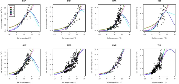
The Exponential and Arrhenius equations overestimated soil respiration at temper-atures below 10◦C in all datasets (Fig. 1). Lloyd-Taylor generally performed better not

15

showing an overestimation at lower temperatures. At five sites, the Gaussian and Van’t Ho_ff equations yielded a maximum in the temperature range of 15–25◦_{C , but}

they provided the best estimates below 10◦C C. Because the maximum was located at rather low temperatures, they tended to underestimate respiration at high temperatures (Fig. 1).

20

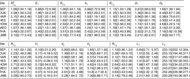
All parameter estimates and their corresponding 99% confidence intervals were significant (P <0.05) except for the first parameter of the Van’t Ho_ff equation (Ap-pendix Table A2). The only parameter estimate directly comparable between the different response functions was the reference respiration, which ranged from 1.06– 1.15 µmol C m−2_s−1_{at the site BEP to 3.49–3.63 µmol C m}−2_s−1_{at the site THA,} re-25

(12)

BGD

6, 8129–8165, 2009

H. Portner et al.

Title Page

Tables Figures

◭ ◮

Back Close

Full Screen / Esc

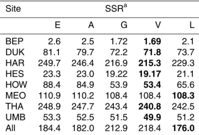
Interactive Discussion The ranking of the performance of the response functions depended on the criterion

used: When the sum of squared residuals was used (Table 3), Van’t Ho_ff performed best (7/8), Gaussian dominated the second rank (5/8) and Lloyd-Taylor dominated the third rank (5/8), but it showed the best fit at the site MEO. When the data for all sites were combined, thus comprising a larger variability of environmental conditions than

5

any site-specific dataset, Lloyd-Taylor showed the best overall fit. The Exponential and Arrhenius formulations generally showed an inferior fit compared to any of the other three equations.

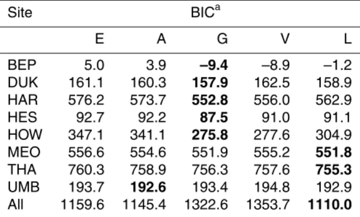
Based on the Bayesian information criterion, i.e. when considering also the number of parameters employed in a given formulation, a lower performance resulted for the

10

Van’t Ho_ff equation as it features the largest number of parameters (Table 4). It now was ranked the second best model at four sites. Best were the Gaussian model at five sites, the Lloyd-Taylor model at two sites and the Arrhenius model at one site. As for the case of the sum of squared residuals, Lloyd-Taylor showed the best performance when all the data were analyzed together, and it was best at two sites, second best at

15

another two sites and third best at the remaining four sites (Table 4).

The uncertainty in the response function according to the sampled parameters showed an increase with increasing temperature (results not shown). As expected, uncertainties increased with the number of parameters used: the Exponential and Ar-rhenius formulations had the lowest uncertainty ranges, Gaussian and Van’t Hoff the

20

highest, and Lloyd-Taylor was characterized by intermediate uncertainty ranges.

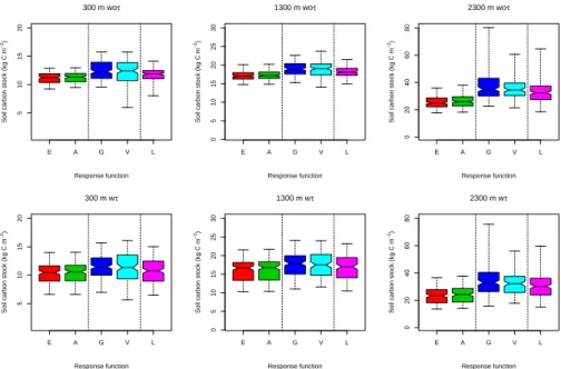
3.2 Long-term carbon stock under present climate

Looking at the carbon stock estimates in 2006, the response functions could be di-vided into the same groups as found in the regression analysis, both according to their median and the magnitude of their uncertainty range (Fig. 2). The results for the

Expo-25

(13)

BGD

6, 8129–8165, 2009

H. Portner et al.

Title Page

Tables Figures

◭ ◮

Back Close

Full Screen / Esc

Interactive Discussion the units of carbon pools are kg C m−2_.

Elevation 300 m: Soil carbon stock estimates for E&A ranged from 9.2–13, for Gaus-sian&Vant’t Ho_ff from 6–15.7 and for Lloyd-Taylor from 8–14.1 when the uncertainty in turnover times was not included. The uncertainty ranges of G&V and Lloyd-Taylor were a factor 2.5 and 1.6 higher than those of the E&A formulations (Fig. 2). When the

5

uncertainty in turnover times (wτ) was considered as well (Fig. 2), uncertainty ranges generally increased. The di_fferences between the groups decreased, however, as the medians were more similar. In addition, the uncertainty range differed less between the groups G&V vs. Lloyd-Taylor, amounting to 1.4 and 1.2 times the uncertainty range of the E&A formulations, respectively (Fig. 2). The response functions E&A showed

10

a strong increase in the uncertainty when the uncertainty in the turnover times of the carbon pools was considered in the analysis.

Elevation 1300 m: The E&A formulations yielded soil carbon stocks in the range of 14.8–20.2, whereas G&V as well as Lloyd-Taylor showed a larger range of 14.1–23.7 and 15–21.5, respectively (Fig. 2). The uncertainty ranges of G&V and Lloyd-Taylor

15

amounted to 1.8 and 1.2 times the range of E&A. When the uncertainty in turnover times was considered additionally, median values differed only little (0.35 kg C m−2), but the uncertainty ranges were much larger (2.1, 1.4 and 2.0 times) for E&A, Gaus-sian&Van’t Ho_ffand Lloyd-Taylor, respectively (Fig. 2).

Elevation 2300 m: At the highest elevation, soil carbon stocks were generally largest

20

and showed a much larger range compared to lower elevation sites. Projections ranged from 17.7–38, from 21.4–80.4 and from 18.5–64.6 for E&A, G&V and Lloyd-Taylor, re-spectively (Fig. 2). For the case wτ we found ranges of 13.6–37.7, 15.8–75.8 and 15.1–59.7, respectively (Fig. 2). When the uncertainty in turnover times was consid-ered, the median carbon stock was 1.6 kg C m−2_{lower. In contrast to the other two} 25

elevations, the range of carbon stock predictions was almost unaffected by the uncer-tainty in turnover times.

(14)

BGD

6, 8129–8165, 2009

H. Portner et al.

Title Page

Tables Figures

◭ ◮

Back Close

Full Screen / Esc

Interactive Discussion elevation site for all model formulations.

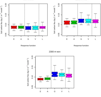
3.3 Short-term carbon flux under present climate

The total carbon fluxes to the atmosphere for casewτ do not directly depend on the turn-over times of the carbon pools, but instead on the size of the carbon pools (results not shown), we therefore report only for the casewoτ. If not differently stated, units of

5

monthly carbon fluxes in August are given in kg C m−2_month−1_.

Elevation 300 m: Soil carbon fluxes for all response functions ranged between 0.06 and 0.11 (Fig. 3), whereby the range was somewhat smaller for the E&A functions. The uncertainty ranges of G&V and Lloyd-Taylor were 1.4 and 1.5 times larger relative to the range of E&A.

10

Elevation 1300 m: On 1300 m elevation the median values were rather similar rang-ing from 0.087 to 0.161 (Fig. 3), although the uncertainty range was larger for the Gaussian and the Lloyd-Taylor function.

Elevation 2300 m: While carbon fluxes increased from 300 to 1300 m, they de-creased again up to 2300 m and three distinct subgroups were identifiable: E&A with a

15

range of 0.076–0.105, G&V with a range of 0.082–0.159, and Lloyd-Taylor with a range of 0.078–0.145 (Fig. 3). This resulted in uncertainty ranges for G&V and Lloyd-Taylor that were 2.7 and 2.3 times the range of E&A.

Changes with elevation: The medians of monthly respiration showed a bell-shaped curve over the elevation gradient, starting with low values at 300 m, inflecting at around

20

1300 m and then decreasing again up to 2300 m. Although the means always were in the range of 0.1_±0.02 kg C m−2_month−1_{, the uncertainty ranges increased steadily} with elevation, particularly for the response functions G&V and Lloyd-Taylor, leading to uncertainty ranges at 2300 m that were 1.5 and 1.7 times larger than the range at 300 m.

(15)

BGD

6, 8129–8165, 2009

H. Portner et al.

Title Page

Tables Figures

◭ ◮

Back Close

Full Screen / Esc

3.4 Long-term carbon stock under future climate

The uncertainty in potential loss of soil carbon due to climate warming (SRES A2 sce-nario, difference between values from 2106 and 2006) was most pronounced at higher elevations (Fig. 4). The same patterns as under current climate were evident for the candidate functions, and hence they are not shown separately.

5

The standard implementation of LPJ-GUESS (with the Lloyd-Taylor formulation) projects a loss of up to 5 kg C m−2_{due to climate change over the whole elevation}

gradient. Accounting for the overall uncertainty in response function, site and turn-over times, the uncertainty in loss of carbon readily increased with elevation, ranging from 1.9 kg C m−2_{at 300 m up to 15.3 kg C m}−2_{at 2300 m, thus leading to highly uncertain} 10

projections at higher elevations. The uncertainty ranges in the projection of soil carbon loss at 1300 m and 2300 m amounted to 3.1 and 8 times the range at 300 m, respec-tively.

4 Discussion

The explanatory power of model outputs heavily depends on the associated

uncer-15

tainty. Models often consist of many functions whose parameters are estimated e.g. us-ing regression analysis based on experimental data. The parameters thus do not have one ’true’ value, but they are characterized by an uncertainty band. The error based on the uncertainty will propagate through the model and lead to a corresponding uncer-tainty in model output (Jones et al., 2003). Di_fferent process formulations and di_fferent

20

parameter sets of the SOM decomposition dynamics may lead to di_fferent model re-sults and therefore may have consequences for the applicability of model projections.

4.1 Fit of the functions

The response functions could be assigned into three groups: exponential&Arrhenius, Gaussian&Van’t Ho_ffand Lloyd-Taylor. Both Exponential and Arrhenius overestimated

(16)

BGD

6, 8129–8165, 2009

H. Portner et al.

Title Page

Tables Figures

◭ ◮

Back Close

Full Screen / Esc

Interactive Discussion the temperature response at low (<10◦_{C ) temperatures, which resulted in an overall}

in-su_fficient fit, thus corroborating the results of earlier research (Lloyd and Taylor, 1994). The Exponential function, which is based on a constantQ₁₀ value is not adequate as theQ₁₀ value has been shown to decrease with increasing temperature (Kirschbaum, 1995). Nevertheless, the Exponential function was included in the analysis because

5

the usage ofQ₁₀ values is still common.

For the other three functions, the rankings di_ffered depending on the criterion em-ployed. As expected, the Van’t Ho_fffunction ranked best when considering the summed square residuals, as it has the largest number of parameters. When we used the Bayesian information criterion, which evaluates the model fit relative to the number

10

of parameters, the Gaussian and Lloyd-Taylor functions performed better. The good performance of the Gaussian function is in line with results from agricultural and for-est soils in Finland and Sitka spruce plantations in Scotland (Tuomi et al., 2008). The Lloyd-Taylor function has been reported to give good results for a variety of soil types (Lloyd and Taylor, 1994) and it is widely used in soil and ecosystem models (Adair

15

et al., 2008; Kucharik et al., 2000; Thornton et al., 2002).

Although the Gaussian and Lloyd-Taylor functions feature the same number of pa-rameters, the Gaussian formulation outperformed the Lloyd-Taylor function by match-ing more of the eight datasets used in this study, which is in line with findmatch-ings by Tuomi et al. (2008). Importantly, when all individual sites were combined, Lloyd-Taylor

out-20

performed both Gaussian and Van’t Hoff with respect to a ranking based on both the summed-squared-residuals and the Bayesian information criterion. As we found that both Gaussian and Van’t Ho_ffunderestimate the response at higher temperatures, we conclude that the decrease of respiration rates at high temperatures was mainly an artefact of model parameterisation. A decline in respiration rates would be expected at

25

(17)

BGD

6, 8129–8165, 2009

H. Portner et al.

Title Page

Tables Figures

◭ ◮

Back Close

Full Screen / Esc

Interactive Discussion function is to be applied over a broad temperature spectrum (Friedlingstein et al., 2006).

The higher the number of parameters there were in a given function, the more in-creased the uncertainty range of the overall parameter space. Although each addi-tional parameter improved the curve fit significantly, it also contributed up to the total uncertainty for the given response function. Gaussian and Van’t Ho_ffhave three and

5

four parameters, respectively, and both show a decline of the response at higher tem-peratures. Functions that do not have this decline at high temperatures, such as Ex-ponential, Arrhenius or Lloyd-Taylor, would have to be complemented by an additional function at very high temperatures to cover respiration decline due to protein denatu-ration. However, based on our data sets there are not enough data points to provide a

10

good estimate of the maximum point, we therefore neither have a reliable estimation of the decline of Van’t Ho_ffand Gaussian directly nor of an additional declining function for Exponential, Arrhenius or Lloyd-Taylor.

Generally, the uncertainty of the response functions increased with higher tempera-tures, because most data points of the eight study sites were highly scattered at higher

15

temperatures. Due to their better explanatory power, one would be tempted to choose the Gaussian or Van’t Hoff response function. However, as the functions were opti-mized using a dataset that comprises temperate test sites only, they would need to be verified over a larger temperature range. Hence, when applying such functions particu-larly for warmer conditions (subtropical and tropical) in the context of global vegetation

20

modelling e_fforts, they are likely to have an unsatisfactory performance. In our test region, even the site with the highest annual mean temperature (at 300 m on our ele-vation gradient), soil temperatures of 20◦_{C were exceeded on average on only 10% of}

the days per year. For sites at higher elevations and hence lower temperatures, soil temperatures never reached the values where the response function had the highest

25

(18)

BGD

6, 8129–8165, 2009

H. Portner et al.

Title Page

Tables Figures

◭ ◮

Back Close

Full Screen / Esc

Interactive Discussion We have to bear in mind however, that measured data at each individual site may

be influenced by additional factors, such as soil moisture conditions (Cisneros-Dozal et al., 2006), litter chemistry (Berg and Laskowski, 2005b) and soil quality (Conant et al., 2008). Still, the regression analysis based on the compound data set shows, that the default response function of Lloyd-Taylor in LPJ-GUESS is worth considering

5

for further work. These findings are in agreement with those by Adair et al. (2008), which found that the function of Lloyd-Taylor performed best with a three-pool model on the Long-term Intersite Decomposition Experiment Team (LIDET) data set. But the findings are in contrast to those by Tuomi et al. (2008), which found the Gaussian function to be best on incubation measurements from different sources.

10

In summary, Arrhenius and Exponential showed poor fits and should not be consid-ered in predictive models. Van’t Ho_ff, the most complex function, showed a good fit, but it had a high uncertainty in parameter estimates. Gaussian and Lloyd-Taylor showed the best fit at individual sites. With the data sets used here, however, reliable estima-tions for the high temperature range can be obtained only when using the Lloyd-Taylor

15

response function.

4.2 Long-term carbon stock under present climate

At low elevations and high temperatures, carbon pools turned over relatively quickly and therefore large carbon stocks did not accumulate, whereas the carbon pools at higher elevations tend to be higher; this is reflected in our simulation results, and it also

20

agrees with experimental findings (Rodeghiero and Cescatti, 2005; Zinke and Stan-genberger, 2000), but disagrees with those of Perruchoud et al. (2000).

The uncertainty bounds of total soil carbon stocks generally increased with elevation, i.e. they decreased with mean temperature for all response functions and sites. At first sight, this may appear counter-intuitive as the uncertainty of the response function

25

(19)

BGD

6, 8129–8165, 2009

H. Portner et al.

Title Page

Tables Figures

◭ ◮

Back Close

Full Screen / Esc

Interactive Discussion readily decomposed and no large soil carbon pools are formed. It is important to take

into account that the accumulation of uncertainty was larger the slower the average decomposition rate became. This was illustrated by the result that the influence of the uncertainty in estimations of the turnover times diminished with increasing elevations. An additional change in an already very low decomposition rate did have only minor

5

e_ffects on the estimations of carbon storage.

At high elevations and hence lower mean temperatures, the uncertainty in decompo-sition rates was relatively small, but it accumulated over time as decompodecompo-sition rates were rather low and thus large carbon pools formed.

In summary, the uncertainty in the projection of long-term soil carbon stocks was

10

considerable both at high and low temperatures in the prevailing model formulations of soil carbon dynamics, but the reasons di_ffered for the two cases depending on the temperature regime. At lower temperatures and thus at higher elevations and latitudes, the high uncertainty was a result of an accumulated uncertainty building up the carbon stock, because carbon pools turn over slowly.

15

At higher temperatures and thus at lower elevations, uncertainty in long-term soil carbon stocks resulted from the uncertainties in temperature response functions itself. Due to high turnover rates, only little carbon accumulated and therefore uncertainty in carbon stock estimations was comparatively low. This may nevertheless be important for tropical and subtropical ecosystems. This has previously been shown by Holland

20

et al. (2000) by using di_fferent temperature sensitivities for tropical decomposition in the Century model.

4.3 Short-term carbon flux under present climate

The short-term fluxes summed over the month of August 2006 showed a more diverse picture along the elevation gradient than the long-term carbon pools. As the carbon flux

25

(20)

BGD

6, 8129–8165, 2009

H. Portner et al.

Title Page

Tables Figures

◭ ◮

Back Close

Full Screen / Esc

Interactive Discussion The carbon pools and their uncertainty increased with elevation, the response

func-tion uncertainty in turn decreased with rising elevafunc-tion and decreasing temperature. The fact that the carbon fluxes increased up to middle and higher elevations and then started to decrease again lead to the conclusion that the sensitivity of the carbon fluxes changed from being more sensitive to carbon pool size at low elevations to being more

5

sensitive to the response function itself at high elevations. This is analogous to Atkin and Tjoelker (2003), who found that the temperature dependence of plant respiration is limited by enzyme activity at low temperatures and by substrate availability at high temperatures.

4.4 Long-term carbon stock under future climate

10

With a climate warming scenario, the carbon pools on all elevation levels turned over faster and the carbon stocks therefore were projected to diminish in the next 100 years, as previously suggested by Jones et al. (2005) and Friedlingstein et al. (2006). How-ever, the high uncertainty in the size of soil carbon pools at higher elevations (i.e. in colder areas) resulted in highly uncertain projections on the net release of carbon from

15

these areas. Therefore, the uncertainty in potential carbon loss from soils in temperate and cold climates is higher than for warmer regions. The higher uncertainty regarding the carbon storage potential of high altitude and high latitude soils adds up to the higher temperature sensitivity of the non-labile soil organic matter pools, as reported by Knorr et al. (2005). Taking into account that high-latitude soils contain large amounts of

car-20

bon whose respiration could cause a significant positive feedback to climate change (Davidson and Janssens, 2006), the uncertainty we found for the projections from LPJ-GUESS for exactly these conditions calls for caution in the interpretation of earlier modeling studies (Friedlingstein et al., 2006), and it clearly calls for further research in this regard.

25

(21)

BGD

6, 8129–8165, 2009

H. Portner et al.

Title Page

Tables Figures

◭ ◮

Back Close

Full Screen / Esc

Interactive Discussion sensitive to increasing temperature. Although this is likely to be true for the response

of the decomposition process to temperature itself, we showed that due to the higher uncertainties in soil carbon pool size in temperate and boreal regions, the relative im-portance of carbon released from soil in a changing climate from the tropics vs. colder ecosystems should be reconsidered.

5

5 Conclusions

The function of Lloyd-Taylor turned out to be adequate for modelling the temperature dependency of soil organic matter decomposition in LPJ-GUESS. The other functions where not as favorable, because they either resulted in poor fits (Exponential, Arrhe-nius) or were not applicable for the given datasets (Gaussian, Van’t Hoff).

10

There were two main sources of uncertainty for model simulations: On the one hand, there was the uncertainty in the parameter estimates of the response functions which increased with decreasing elevation. On the other hand, there was the resulting un-certainty in the simulation of carbon pools and fluxes which increased with elevation, as soil carbon at low elevations was readily degraded due to faster turn-over times, but

15

the slower turn-over times at high elevations lead to higher carbon stocks and higher associated uncertainties. The higher uncertainty in carbon pools with slow turn-over rates has important implications for the uncertainty in the projection of the change of soil carbon stocks driven by climate change, which turned out to be more uncertain for higher elevations and hence higher latitudes, which are of key importance for the

20

global terrestrial carbon budget.

Acknowledgements. This work was supported by grant no. TH-14 07-1 of ETH Z ¨urich and by the National Centre of Competence in Climate Research (NCCR Climate), Switzerland.

Climate and CO2data were provided through the PRUDENCE data archive, funded by the EU

(22)

BGD

6, 8129–8165, 2009

H. Portner et al.

Title Page

Tables Figures

◭ ◮

Back Close

Full Screen / Esc

References

Adair, E. C., Parton, W. J., Grosso, S. J. D., Silver, W. L., Harmon, M. E., Hall, S. A., Burke, I. C., and Hart, S. C.: Simple three-pool model accurately describes patterns of long-term litter decomposition in diverse climates, Global Change Biol., 14, 2636–2660, 2008. 8144, 8146

5 ˚

Agren, G. I. and Bosatta, N.: Theoretical analysis of the long-term dynamics of carbon and nitrogen in soils, Ecology, 68, 1181–1189, 1987. 8131

Atkin, O. K. and Tjoelker, M. G.: Thermal acclimation and the dynamic response of plant respi-ration to temperature, Trends in Plant Science, 8, 343–351, 2003. 8148

Berg, B. and Laskowski, R.: Anthropogenic impacts on litter decomposition and soil organic 10

matter, Adv. Ecol. Res., 38, 263–290, 2005a. 8131

Berg, B. and Laskowski, R.: Climatic and Geographic Patterns in Decomposition, Adv. Ecol. Res., 38, 227–261, 2005b. 8131, 8146

Bosatta, E. and ˚Agren, G. I.: Soil organic matter quality interpreted thermodynamically, Soil

Biol. Biochem., 31, 1889–1891, 1999. 8131 15

Bronson, D. R., Gower, S. T., Tanner, M., Linder, S., and Herk, I. V.: Response of soil surface CO2 flux in a boreal forest to ecosystem warming, Global Change Biol., 14, 856–867, 2008. 8131

Christensen, J., Carter, T., Rummukainen, M., and Amanatidis, G.: Evaluating the performance and utility of regional climate models: the PRUDENCE project, Clim. Change, 81, 1–6, 2007. 20

8138

Cisneros-Dozal, L. M., Trumbore, S., and Hanson, P. J.: Partitioning sources of soil-respired CO2 and their seasonal variation using a unique radiocarbon tracer, Global Change Biol., 12, 194–204, 2006. 8131, 8146

Conant, R. T., Drijiber, R. A., Haddix, M. L., Parton, W. J., Paul, E. A., Plante, A. F., Six, J., 25

and Steinweg, J. M.: Sensitivity of organic matter decomposition to warming varies with its quality, Global Change Biol., 14, 868–877, 2008. 8146

Cornwell, W. K., Cornelissen, J. H. C., Amatangelo, K., Dorrepaal, E., Eviner, V. T., Godoy, O., Hobbie, S. E., Hoorens, B., Kurokawa, H., P ´erez-Harguindeguy, N., Quested, H. M., Santiago, L. S., Wardle, D. A., Wright, I. J., Aerts, R., Allison, S. D., van Bodegom, P., 30

Brovkin, V., Chatain, A., Callaghan, T. V., D´ıaz, S., Garnier, E., Gurvich, D. E., Kazakou, E.,

(23)

BGD

6, 8129–8165, 2009

H. Portner et al.

Title Page

Tables Figures

◭ ◮

Back Close

Full Screen / Esc

Plant species traits are the predominant control on litter decomposition rates within biomes worldwide, Ecol. Lett., 11, 1065–1071, 2008. 8131

Cramer, W., Bondeau, A., Woodward, F. I., Prentice, I. C., Betts, R. A., Brovkin, V., Cox, P. M., Fisher, V., Foley, J. A., Friend, A. D., Kucharik, C., Lomas, M. R., Ramankutty, N., Sitch, S., Smith, B., White, A., and Young-Molling, C.: Global response of terrestrial ecosystem 5

structure and function to CO2 and climate change: results from six dynamic global vegetation models, Global Change Biol., 7, 357–373, 2001. 8132, 8133

Davidson, E. A. and Janssens, I. A.: Temperature sensitivity of soil carbon decomposition and feedbacks to climate change, Nature, 440, 165–173, 2006. 8131, 8148

Eliasson, P. E., McMurtrie, R. E., Pepper, D. A., Stromgren, M., Linder, S., and ˚Agren, G. I.:

10

The response of heterotrophic CO2 flux to soil warming, Global Change Biol., 11, 167–181, 2005. 8131

Foley, J. A.: Numerical Models of the Terrestrial Biosphere, J. Biogeogr., 22, 837–842, 1995. 8134

Friedlingstein, P., Cox, P., Betts, R., Bopp, L., von Bloh, W., Brovkin, V., Cadule, P., Doney, S., 15

Eby, M., Fung, I., Bala, G., John, J., Jones, C., Joos, F., Kato, T., Kawamiya, M., Knorr, W., Lindsay, K., Matthews, H. D., Raddatz, T., Rayner, P., Reick, C., Roeckner, E., Schnitzler, K., Schnur, R., Strassmann, K., Weaver, A. J., Yoshikawa, C., and Zeng, N.: Climate–Carbon Cycle Feedback Analysis: Results from the C4MIP Model Intercomparison, J. Climate, 19, 3337–3353, 2006. 8132, 8145, 8148

20

Hakkenberg, R., Churkina, G., Rodeghiero, M., B ¨orner, A., Steinhof, A., and Cescatti, A.: Temperature sensitivity of the turnover times of soil organic matter in forests, Ecol. Appl., 18, 119–31, 2008. 8131

Hibbard, K., Law, B., Reichstein, M., and Sulzman, J.: An analysis of soil respiration across northern hemisphere temperate ecosystems, Biogeochemistry, 73, 29–70, 2005. 8133 25

Hibbard, K., Hudiburg, T., Law, B., Reichstein, M., and Sulzman, J.: Northern Hemisphere Temperate Ecosystem Annual Soil Respiration Data (from Hibbard et al. 2005. An analy-sis of soil respiration across northern hemisphere temperate ecosystems. Biogeochemistry 73, 29–70), accessed 03-01-2008 at: ftp://cdiac.ornl.gov/pub/ameriflux/data/synthesis-data/ soil respiration Hibbard/, 2006. 8133, 8135, 8156

30

Holland, E. A., Neff, J. C., Townsend, A. R., and McKeown, B.: Uncertainties in the temperature

(24)

BGD

6, 8129–8165, 2009

H. Portner et al.

Title Page

Tables Figures

◭ ◮

Back Close

Full Screen / Esc

Iman, R. L. and Conover, W. J.: A distribution-free approach to inducing rank correlation among input variables, Communications in Statistics – Simulation and Computation, 11, 311–334, 1982. 8137

Jones, C., McConnell, C., Coleman, K., Cox, P., Falloon, P., Jenkinson, D., and Powlson, D.: Global climate change and soil carbon stocks; predictions from two contrasting models for 5

the turnover of organic carbon in soil, Global Change Biol., 11, 154–166, 2005. 8148 Jones, C. D., Cox, P., and Huntington, C.: Uncertainty in climate carbon-cycle projections

associated with the sensitivity of soil respiration to temperature, Tellus B, 55, 642–648, 2003. 8143

Kirschbaum, M. U. F.: The temperature dependence of soil organic matter decomposition, and 10

the effect of global warming on soil organic C storage, Soil Biol. Biochem., 27, 753–760,

1995. 8144

Kirschbaum, M. U. F.: Soil respiration under prolonged soil warming: are rate reductions caused by acclimation or substrate loss?, Global Change Biol., 10, 1870–1877, 2004. 8131

Kirschbaum, M. U. F.: The temperature dependence of organic-matter decomposition–still a 15

topic of debate, Soil Biol. Biochem., 38, 2510–2518, 2006. 8131

Knorr, W., Prentice, C. I., House, J. I., and Holland, E. A.: Long-term sensitivity of soil carbon turnover to warming, Nature, 433, 298–301, 2005. 8131, 8148

Kucharik, C. J., Foley, J. A., Delire, C., Fisher, V. A., Coe, M. T., Lenters, J. D., Young-Molling, C., Ramankutty, N., Norman, J. M., and Gower, S. T.: Testing the Performance of a Dynamic 20

Global Ecosystem Model: Water Balance, Carbon Balance, and Vegetation Structure, Global Biogeochem. Cy., 14, 795–825, 2000. 8144

Larcher, W.: ¨Okophysiologie der Pflanzen, Verlag Eugen Ulmer, Stuttgart, 6. neubearbeitete

auflage edn., 2001. 8144

Lloyd, J. and Taylor, J. A.: On the Temperature Dependence of Soil Respiration, Functional 25

Ecology, 8, 315–323, 1994. 8133, 8134, 8144

Meentemeyer, V.: Macroclimate the Lignin Control of Litter Decomposition Rates, Ecology, 59, 465–472, 1978. 8134

Mitchell, T. D., Mitchell, T. D., Carter, T. R., Jones, P. D., Hulme, M., and New, M.: A comprehen-sive set of climate scenarios for Europe and the globe., Tyndall Centre for Climate Change 30

Research Working Paper, 2003. 8138

(25)

BGD

6, 8129–8165, 2009

H. Portner et al.

Title Page

Tables Figures

◭ ◮

Back Close

Full Screen / Esc

model predictions of carbon and water fluxes in major European forest biomes, Global Change Biol., 11, 2211–2233, 2005. 8133

Morales, P., Hickler, T., Rowell, D. P., Smith, B., and Sykes, M. T.: Changes in European Ecosys-tem Productivity and Carbon Balance Driven by Regional Climate Model Output, Global Change Biol., 13, 108–122, 2007. 8133

5

O’Connell, A. M.: Microbial decomposition (respiration) of litter in eucalypt forests of South-Western Australia: An empirical model based on laboratory incubations, Soil Biol. Biochem., 22, 153–160, 1990. 8133, 8135

Parton, W. J., Schimel, D. S., Cole, C. V., and Ojima, D. S.: Analysis of factors controlling soil organic matter levels in Great Plains grasslands, Soil Science Society of America Journal, 10

51, 1173–1179, 1987. 8137

Perruchoud, D., Walthert, L., Zimmermann, S., and L ¨uscher, P.: Contemporary carbon stocks of mineral forest soils in the Swiss Alps, Biogeochemistry, 50, 111–136, 2000. 8146

R Development Core Team: R: A Language and Environment for Statistical Computing, Vienna, Austria, 2008. 8136

15

Ratkowsky, D. A.: Handbook of Nonlinear Regression Models, in: Statistics: Textbooks and Monographs, Marcel Dekker, Inc., New York, 1990. 8136, 8159

Rodeghiero, M. and Cescatti, A.: Main determinants of forest soil respiration along an ele-vation/temperature gradient in the Italian Alps, Global Change Biol., 11, 1024–1041, 2005. 8146

20

Saltelli, A., Tarantola, S., Campolongo, F., and Ratto, M.: Sensitivity analysis in practice – a guide to assessing scientific models, John Wiley & Sons, Ltd., Chichester, 2004. 8137 Schlesinger, W. H.: Biogeochemistry: an Analysis of Global Change, Academic Press, San

Diego, second edn., 1997. 8131

Schwarz, G.: Estimating the Dimension of a Model, The Annals of Statistics, 6, 461–464, 1978. 25

8136, 8158

Sitch, S., Smith, B., Prentice, I. C., Arneth, A., Bondeau, A., Cramer, W., Kaplan, J. O., Levis, S., Lucht, W., Sykes, M. T., Thonicke, K., and Venevsky, S.: Evaluation of ecosystem dynamics, plant geography and terrestrial carbon cycling in the LPJ dynamic global vegetation model, Global Change Biol., 9, 161–185, 2003. 8133, 8138

30

(26)

BGD

6, 8129–8165, 2009

H. Portner et al.

Title Page

Tables Figures

◭ ◮

Back Close

Full Screen / Esc

Solomon, S., Qin, D., Manning, M., Chen, Z., Marquis, M., Averyt, K., M.Tignor, and Miller, H.: IPCC, 2007: Summary for Policymakers, Cambridge University Press, Cambridge, United Kingdom and New York, NY, USA, 2007. 8131

Thornton, P. E., Running, S. W., and White, M. A.: Generating surfaces of daily meteorological variables over large regions of complex terrain, J. Hydrol., 190, 214–251, 1997. 8137 5

Thornton, P. E., Law, B. E., Gholz, H. L., Clark, K. L., Falge, E., Ellsworth, D. S., Goldstein, A. H., Monson, R. K., Hollinger, D., Falk, M., Chen, J., and Sparks, J. P.: Modeling and

measuring the effects of disturbance history and climate on carbon and water budgets in

evergreen needleleaf forests, Agr. Forest Meteorol., 113, 185–222, 2002. 8144

Townsend, A. R., Vitousek, P. M., and Holland, E. A.: Tropical soils could dominate the short-10

term carbon cycle feedbacks to increased global temperatures, Clim. Change, 22, 293–303, 1992. 8148

Tuomi, M., Vanhala, P., Karhu, K., Fritze, H., and Liski, J.: Heterotrophic soil respiration–

Comparison of different models describing its temperature dependence, Ecol. Modelling,

211, 182–190, 2008. 8133, 8135, 8144, 8146 15

Van’t Hoff, J. H.: Vorlesungen ¨uber theoretische und physicalische Chemie. Erstes Heft: Die

chemische Dynamik, Druck und Verlag von Friedrich Vieweg und Sohn, Braunschweig, 1901. 8133, 8134

Weedon, J. T., Cornwell, W. K., Cornelissen, J. H., Zanne, A. E., Wirth, C., and Coomes, D. A.: Global meta-analysis of wood decomposition rates: a role for trait variation among 20

tree species?, Ecol. Lett., 12, 45–56, 2009. 8131

(27)

BGD

6, 8129–8165, 2009

H. Portner et al.

Title Page

Tables Figures

◭ ◮

Back Close

Full Screen / Esc

Interactive Discussion Table 1.Temperature response functions.

Id Differential equation Absolute function Relative functiona

Eb dl nRT

d T =C RT=e

C×T

×Const RT=RTref×e

C×(T−Tref₎

A dl nRT

d T =

A

T2 RT=e

−A_T

×Const R_T=R_T_ref×eA×(Tref1 −

1

T₎

G dl nRT

d T =a+2bT RT=e

aT+bT2

×Const RT=RTref×e

a×(T−Tref)+b×(T 2

−Tref2)

V dl nRT

d T =

A T2 +

B

T +C RT=e−

A T

×TB×eC×T×Const RT=RTref×e

A×( 1

Tref− 1

T)+B×log( T

Tref)+C×(T−Tref)

L dl nRT

d T =

A

(T−T0)2

R_T=e−T−AT0_×Const R

T=RTref×e

A×( 1

Tref−T0− 1

T−T0)

a

Functions expressed relative to reference temperature T_ref=10◦_{C with reference respiration}

R_T

ref normalized to 1 at mean reference respirationRTref.

b

The candiate functions are:

(28)

BGD

6, 8129–8165, 2009

H. Portner et al.

Title Page

Tables Figures

◭ ◮

Back Close

Full Screen / Esc

Interactive Discussion Table 2.Site characteristics.

Site Description Location Elevation (m) MATa Nb Forest vegetation type

BEP Belgium de Inslag Pine 51.31N 4.31E 16 10 41 Evergreen-needleleaf DUK Duke FACE 35.97N 79.1W 120–163 15.5 47 Evergreen-needleleaf HAR Harvard 42.54N 72.17W 180–490 7.85 197 Mixed Deciduous-evergreen

HES Hesse 48.67N 7.08E 300 9.7 39 Deciduous-broadleaf

HOW Howland 45.2N 68.7W 60 5.69 164 Evergreen-neddleleaf MEO Metolius old site 44.5N 121.62W 915–1141 8.5 316 Evergreen-needleleaf THA Tharandt 50.96N 13.75E 380 7.6 279 Evergreen–eedleleaf UMB Univ. of Michigan Biological Station 45.56N 84.71W 234 6.2 78 Mixed Deciduous-evergreen

(29)

BGD

6, 8129–8165, 2009

H. Portner et al.

Title Page

Tables Figures

◭ ◮

Back Close

Full Screen / Esc

Interactive Discussion Table 3.Summed squared residuals of nonlinear model fits.

Site SSRa

E A G V L

BEP 2.6 2.5 1.72 1.69 2.1

DUK 81.1 79.7 72.2 71.8 73.7

HAR 249.7 246.4 216.9 215.3 229.3

HES 23.3 23.0 19.22 19.17 21.1

HOW 88.4 84.9 53.9 53.4 65.6

MEO 110.9 110.2 108.4 108.4 108.3

THA 248.9 247.7 243.4 240.8 242.5

UMB 53.3 52.5 51.5 49.9 51.2

All 184.4 182.0 212.9 218.4 176.0

a

SSR: Summed Squared Residuals. Best (lowest) values for each site shown in bold numbers.

(30)

BGD

6, 8129–8165, 2009

H. Portner et al.

Title Page

Tables Figures

◭ ◮

Back Close

Full Screen / Esc

Interactive Discussion Table 4.Ranking of nonlinear model fits.

Site BICa

E A G V L

BEP 5.0 3.9 –9.4 –8.9 –1.2

DUK 161.1 160.3 157.9 162.5 158.9

HAR 576.2 573.7 552.8 556.0 562.9

HES 92.7 92.2 87.5 91.0 91.1

HOW 347.1 341.1 275.8 277.6 304.9

MEO 556.6 554.6 551.9 555.2 551.8

THA 760.3 758.9 756.3 757.6 755.3

UMB 193.7 192.6 193.4 194.8 192.9

All 1159.6 1145.4 1322.6 1353.7 1110.0

a

BIC: Bayesian information criterion (Schwarz, 1978). Best (lowest) values for each site shown

(31)

BGD

6, 8129–8165, 2009

H. Portner et al.

Title Page

Tables Figures

◭ ◮

Back Close

Full Screen / Esc

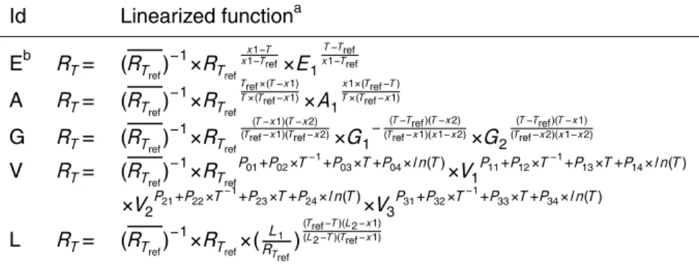
Interactive Discussion Table A1.Linearized temperature response functions.

Id Linearized functiona

Eb R_T= (R_T_ref)−1

×R_T_refxx1−1−TTref_×E

1

T−Tref

x1−Tref

A R_T= (R_T

ref)

−1

×RTref

Tref×(T−x1)

T×(Tref−x1) ×A1

x1×(Tref−T)

T×(Tref−x1)

G R_T= (R_T

ref)

−1

×RTref

(T−x1)(T−x2) (Tref−x1)(Tref−x2)

×G1

−(T(Tref−−Tref )(x1)(Tx1−−x2)x2) ×G2

(T−Tref )(T−x1) (Tref−x2)(x1−x2)

V R_T= (R_T

ref)

−1

×RTref

P01+P02×T− 1

+P03×T+P04×l n(T) ×V1

P11+P12×T− 1

+P13×T+P14×l n(T) ×V2

P21+P22×T−1

+P23×T+P24×l n(T)

×V3

P31+P32×T−1

+P33×T+P34×l n(T)

L R_T= (R_T

ref)

−1

×RTref×(

L1

RTref

)

(Tref−T)(L2−x1) (L2−T)(Tref−x1)

a

Temperature response functions linearized with the method of expected-value parameters

(Ratkowsky, 1990). T_ref=283.15 K,×0=268.15 K (for V only), ×1=280.15 K, ×2=292.15 K. b

The candiate functions are: Exponential (E), Arrhenius (A), Gaussian (G), Van’t Hoff(V) and

(32)

BGD

6, 8129–8165, 2009

H. Portner et al.

Title Page

Tables Figures

◭ ◮

Back Close

Full Screen / Esc

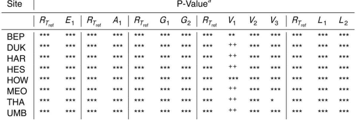
Interactive Discussion Table A2.Significance levels.

Site P-Valuea

R_T

ref E1 RTref A1 RTref G1 G2 RTref V1 V2 V3 RTref L1 L2

BEP *** *** *** *** *** *** *** *** ** *** *** *** *** ***

DUK *** *** *** *** *** *** *** *** ++ *** *** *** *** ***

HAR *** *** *** *** *** *** *** *** ++ *** *** *** *** ***

HES *** *** *** *** *** *** *** *** ++ *** *** *** *** ***

HOW *** *** *** *** *** *** *** *** *** *** *** *** *** ***

MEO *** *** *** *** *** *** *** *** ++ *** *** *** *** ***

THA *** *** *** *** *** *** *** *** ++ *** * *** *** ***

UMB *** *** *** *** *** *** *** *** ++ *** *** *** *** ***

Significance levels are given in P-Values for all the parameters of nonlinear model fits for each pair of temperature response function (as given in Appendix Table A1) and calibration site.

a