Monitoring and modelling of soil–plant interactions: the joint use of ERT, sap flow and Eddy Covariance data to characterize the volume of an orange tree root zone

(1)

HESSD

11, 13353–13384, 2014

Monitoring and modelling of

soil–plant interactions

G. Cassiani et al.

Title Page

Abstract Introduction

Conclusions References

Tables Figures

◭ ◮

Back Close

Full Screen / Esc

Printer-friendly Version Interactive Discussion

Discussion

P

a

per

|

Discussion

P

a

per

|

Discussion

P

a

per

|

Discussion

P

a

per

|

Hydrol. Earth Syst. Sci. Discuss., 11, 13353–13384, 2014 www.hydrol-earth-syst-sci-discuss.net/11/13353/2014/ doi:10.5194/hessd-11-13353-2014

This discussion paper is/has been under review for the journal Hydrology and Earth System Sciences (HESS). Please refer to the corresponding final paper in HESS if available.

Monitoring and modelling of soil–plant

interactions: the joint use of ERT, sap flow

and Eddy Covariance data to characterize

the volume of an orange tree root zone

G. Cassiani1, J. Boaga1, D. Vanella2, M. T. Perri1, and S. Consoli2

1

University of Padua, Department of Geosciences, Padua, Italy

2

University of Catania, Department of Agri-food and Environmental Systems Management, Catania, Italy

Received: 10 October 2014 – Accepted: 15 November 2014 – Published: 8 December 2014 Correspondence to: G. Cassiani ([email protected])

(2)

HESSD

11, 13353–13384, 2014

G. Cassiani et al.

Title Page

Tables Figures

◭ ◮

Back Close

Full Screen / Esc

Discussion

P

a

per

|

Discussion

P

a

per

|

Discussion

P

a

per

|

Discussion

P

a

per

|

Abstract

Mass and energy exchanges between soil, plants and atmosphere control a number of key environmental processes involving hydrology, biota and climate. The understand-ing of these exchanges also play a critical role for practical purposes e.g. in precision agriculture. In this paper we present a methodology based on coupling innovative data

5

collection and models in order to obtain quantitative estimates of the key parameters of such complex flow system. In particular we propose the use of hydro-geophysical monitoring via 4-D Electrical Resistivity Tomography (ERT) in conjunction with mea-surements of plant transpiration via sap flow and evapotranspiration from Eddy Covari-ance (EC). This abundCovari-ance of data is fed to a spatially distributed soil model in order

10

to characterize the distribution of active roots. We conducted experiments in an orange orchard in Eastern Sicily (Italy), characterized by the typical Mediterranean semi-arid climate. The subsoil dynamics, particularly influenced by irrigation and root uptake, were characterized mainly by the ERT setup, consisting of 48 buried electrodes on 4 instrumented micro boreholes (about 1.2 m deep) placed at the corners of a square

15

(about 1.3 m in side) surrounding the orange tree, plus 24 mini-electrodes on the sur-face spaced 0.1 m on a square grid. During the monitoring, we collected repeated ERT and TDR soil moisture measurements, soil water samples, sap flow measurements from the orange tree and EC data. We conducted a laboratory calibration of the soil electrical properties as a function of moisture content and pore water electrical

conduc-20

tivity. Irrigation, precipitation, sap flow and ET data are available allowing knowledge of the system’s long term forcing conditions on the system. This information was used to calibrate a 1-D Richards’ equation model representing the dynamics of the volume monitored via 3-D ERT. Information on the soil hydraulic properties was collected from laboratory and field experiments. The successful results of the calibrated modeling

ex-25

ercise allow the quantification of the soil volume interested by root water uptake. This

volume is much smaller (with a surface area less than 2 m2, and about 40 cm

(3)

HESSD

11, 13353–13384, 2014

G. Cassiani et al.

Title Page

Tables Figures

◭ ◮

Back Close

Full Screen / Esc

Discussion

P

a

per

|

Discussion

P

a

per

|

Discussion

P

a

per

|

Discussion

P

a

per

|

that prove to be losing at least half of the irrigated water that is not uptaken by the plants.

1 Introduction

The system made of soil, vegetation and the adjacent atmosphere is characterized by complex patterns, structures, and processes that act on a wide range of time and

5

space scales. While the exchange of energy and water is continuous between com-partments, the pertinent fluxes are strongly heterogeneous and variable in space and time and this makes their quantification particularly challenging. Plants are known to impact the terrestrial water cycle and underground water dynamics through evapo-transpiration (ET) and root water uptake (RWU). The mechanisms of water flow in the

10

root zone are controlled by soil physics, plant physiology and meteorological factors (Green et al., 2003a). The translation of plant water use strategies into physically-based models of root water uptake is a crucial issue in eco-hydrology and has fundamental consequence in the understanding and modelling of atmospheric as well as soil pro-cesses. Still, no consensus exists on the modelling of this process (Feddes et al., 2001;

15

Raats, 2007). From a conceptual point of view, two main approaches exist today, which

differ in the way of predicting the volumetric rate of RWU.

A first approach expresses water transport in plants as a chain process based on a resistance law. Coupled with a three-dimensional soil water flow model, this approach leads to fairly accurate RWU models at the plant scale (Doussan et al., 2006; Schneider

20

et al., 2010), also under water stress conditions. The limitations of these models are the cost of characterizing parameters, such as root system architecture and conductance to water flow, and their computational demand. A second approach, mostly used in soil-vegetation-atmosphere transfer models, relies on “macroscopic parameters” and predicts RWU as a product of the potential transpiration rate, a spatially distributed

25

(4)

draw-HESSD

11, 13353–13384, 2014

G. Cassiani et al.

Title Page

Tables Figures

◭ ◮

Back Close

Full Screen / Esc

Discussion

P

a

per

|

Discussion

P

a

per

|

Discussion

P

a

per

|

Discussion

P

a

per

|

back of this approach is the necessity to calibrate the macroscopic parameters, which introduces substantial uncertainties (Musters and Bouten, 2000).

The complexity of RWU modelling is highly related to the uneven root distribution in the vertical and radial directions (Gong et al., 2006). This variability is partly induced by heterogeneities in the soil and localized soil compaction caused by both cultivation

5

and irrigation patterns (Jones and Tardieu, 1998) that in turn cause heterogeneous water and nutrient distribution. Consequently, there is a clear need for the development of novel RWU modelling approaches (Feddes et al., 2001; Raats, 2007; Jarvis, 2011; Couvreur et al., 2012), as well as for accurate measurements techniques of soil water content and RWU dynamics.

10

In particular, soil moisture measurements are of paramount importance to calibrate RWU models. Traditionally, and especially beneath irrigated crops, soil moisture has been determined using methods such as neutron probes, TDR or capacitance sys-tems. As these traditional techniques are point measurements, they do not provide suf-ficient information for reliable mass balance assessments; therefore our understanding

15

of RWU as a spatially distributed system remains fundamentally limited. In this respect the understanding of soil as a spatially heterogeneous system shares fundamental lim-itations with most of earth sciences. Therefore much can be learnt looking at similar research fields.

Geophysical methods have long been established for the imaging of the soil

subsur-20

face at a variety of scales, from large scale mining exploration (e.g. Parasnis, 1973) to the very small scale of soil mapping (e.g. Allred et al., 2008). The past twenty years, in particular, have seen the fast development of techniques that are useful in identifying structure and dynamics of the near surface, with particular reference to hydrological applications. This realm of research goes under the general name of hydro-geophysics

25

(5)

HESSD

11, 13353–13384, 2014

G. Cassiani et al.

Title Page

Tables Figures

◭ ◮

Back Close

Full Screen / Esc

Discussion

P

a

per

|

Discussion

P

a

per

|

Discussion

P

a

per

|

Discussion

P

a

per

|

(e.g. Weill et al., 2013) and hillslope characterization (Cassiani et al., 2009) to agricul-ture and eco-hydrological processes (Ursino et al., 2014; Boaga et al., 2014).

Possibly the most interesting results have been obtained when hydro-geophysical data have been coupled with distributed hydrological model predictions. The degree of integration of data and model range from trial and error calibration (e.g. Binley et al.,

5

2002) to full data assimilation (e.g. Hinnell et al., 2010), but in all cases the availability of spatially extensive (and time intensive) data greatly improve the models’ capability to identify within narrow ranges the relevant governing parameters, that in turn are of practical interest for hydrological predictions.

Relatively few hydro-geophysical applications, though, have been focussed on

10

plant root system characterization (e.g. al Hagrey et al., 2007; Javaux et al., 2008; Jayawickreme et al., 2008; Werban et al., 2008; al Hagrey and Petersen, 2011), often limiting the analysis to a tentative identification of the main root location and extent.

In this paper we aim at applying hydro-geophysical techniques, with a combination of measurements and modelling, to a tree root system. This approach has, to the best

15

of our knowledge, not been presented and analysed yet. In particular, we present the application of the time-lapse non-invasive 3-D electrical resistivity tomography (ERT) to monitor soil–plant interactions in the root zone of an orange tree located in the Mediter-ranean semi-arid Sicilian (South Italy) context. The subsoil dynamics, particularly influ-enced by irrigation and RWU, have been characterized by the 3-D ERT measurements

20

coupled with plant transpiration through sap flow measurements. The information con-tained in the ERT measurements in terms of vadose zone water dynamics was ex-ploited by comparing the field results against a 1-D vadose zone model.

The specific goals of this paper are

1. to study the feasibility of a small scale monitoring of root zone processes using

25

time-lapse 3-D ERT;

(6)

HESSD

11, 13353–13384, 2014

G. Cassiani et al.

Title Page

Tables Figures

◭ ◮

Back Close

Full Screen / Esc

Discussion

P

a

per

|

Discussion

P

a

per

|

Discussion

P

a

per

|

Discussion

P

a

per

|

3. to interpret these data with the aid of a physical hydrological model, in order to derive also information on the root zone physical structure and its dynamics.

2 Site description

The Bulgherano experimental site

The experiment was conducted in a 20 ha orange orchard, planted with about 20

year-5

old trees (Citrus sinensis, cv Tarocco Ippolito) (Fig. 1). The field is located in Lentini

(Eastern Sicily, Lat. 37◦16′N, Long. 14◦53′E) in a Mediterranean semi-arid

environ-ment, characterized by an annual average precipitation of around 550 mm, very dry

summers and average air temperature of 7◦_{C in winter and 28}◦_{C in summer. The site}

presents conditions of crop homogeneity, flat slope, dominant wind speed direction for

10

footprint analysis and quite large fetch that are ideal for micrometeorological

measure-ments. The planting layout is 4.0 m×5.5 m and the trees are drip irrigated with 4 in-line

drippers per plant, spaced about 1 m, with 16 L h−1of total discharge (4 L h−1dripper−1);

the crop is well-watered by irrigation supplied every day from May to October, with

ir-rigation timing of 5 h d−1_{. The study area has a mean leaf area index (LAI) of about}

15

4 m2m−2, measured by a LAI-2000 digital analyser (LI-COR, Lincoln, Nebraska, USA).

The mean PAR (photosynthetic active radiation) light interception was 80 % within rows

and 50 % between rows; the canopy height (h_c) is 3.7 m.

The soil characterization was performed via textural and hydraulic laboratory analy-ses, according to the USDA standards, and it is classified as loamy sand. In this study

20

we used van Genuchten’s (1980) analytical expression to describe soil water retention and a falling-head permeameter to determine the hydraulic conductivity at saturation. For each soil sample, the moisture content at standard water potential values was de-termined by a sandbox and a pressure membrane apparatus (Aiello et al., 2014).

Three soil water content profiles are measured in the field using TDR (Time Domine

25

(7)

HESSD

11, 13353–13384, 2014

G. Cassiani et al.

Title Page

Tables Figures

◭ ◮

Back Close

Full Screen / Esc

Discussion

P

a

per

|

Discussion

P

a

per

|

Discussion

P

a

per

|

Discussion

P

a

per

|

(±2.5 % of accuracy) were installed to monitor every 1 h the changes of volumetric soil

water content (∆θ). The TDR probe installation was designed to measure soil water

content variations with time in the soil volume afferent to each plant. For each

loca-tion the TDR equipment consists of two sensors inserted vertically at 0.25 and 0.45 m depth and of two sensors inserted horizontally at 0.35 m depth with 0.20 m in between.

5

The data that are discussed here (see results section) correspond to the TDR probes located at about 1.5 m from the orange tree we monitored with ERT.

Hourly meteorological data (incoming short-wave solar radiation, air temperature, air humidity, wind speed and rainfall) are acquired by an automatic weather station located about 7 km from the orchard and managed by SIAS (Agro-meteorological Service of the

10

Sicilian Region). For the dominant wind directions, the fetch is larger than 550 m. For the other sectors the minimum fetch is 400 m (SE).

3 Methodology

3.1 Micrometeorological measurements

The experimental site is equipped with Eddy Covariance (EC) systems mounted on

15

a micrometeorological fluxes tower (Fig. 1). Continuous energy balance

measure-ments have been since 2009. Net radiation (Rn, W m−

2

) is measured with two CNR 1 Kipp & Zonen (Campbell Scientific Ltd) net radiometers at a height of 8 m. Soil heat

flux density (G, W m−2) is measured with three soil heat flux plates (HFP01, Campbell

Scientific Ltd) placed horizontally 0.05 m below the soil surface. Three different

mea-20

surements ofGwere selected: in the trunk row (shaded area), at 1/3 of the distance to

the adjacent row, and at 2/3 of the distance to the adjacent row. The soil heat flux is

measured as the mean output of three soil heat flux plates. Data from the soil heat flux plates is corrected for heat storage in the soil above the plates.

The air temperature and the three wind speed components are measured at

25

(8)

HESSD

11, 13353–13384, 2014

G. Cassiani et al.

Title Page

Tables Figures

◭ ◮

Back Close

Full Screen / Esc

Discussion

P

a

per

|

Discussion

P

a

per

|

Discussion

P

a

per

|

Discussion

P

a

per

|

anemometers (Windmaster Pro, Gill Instruments Ltd, at 4 m, and a CSAT, Campbell Sci., at 8 m). A gas analyzer (CSAT, Campbell Sci.) operating at 10 Hz was installed at 8 m. The raw data are recorded at a frequency of 10 Hz using two synchronized data loggers (CR3000, Campbell Sci.).

Low frequency measurements are taken for air temperature and humidity (HMP45C,

5

Vaisala), wind speed and direction (05 103 RM Young), and atmospheric pressure (CS106, Campbell Scientific Ltd) at 4, 8 and 10 m.

The freely distributed TK2 package (Mauder and Foken, 2004) is used to determine the first and second order statistical moments and fluxes on a half-hourly basis follow-ing the protocol used as a comparison reference described in Mauder et al. (2007).

10

Surface energy balance measurements at the experimental site show that the sum of

sensible and latent (LE) heat flux is highly correlated (r2>0.90) (Fig. 2) to the sum of

net radiation and soil heat flux (Castellvì et al., 2012; Consoli and Papa, 2013). A linear fit between the two quantities show a certain energy balance un-closure. The percent-age of un-closure (about 10 %) is in the range reported by most flux sites (Wilson et al.,

15

2002) and provides additional confirmation of the turbulent flux quality (Moncrieffet al.,

2004).

3.2 Sap flow measurements

Measurements of water consumption at tree level (TSF) are taken using the HPV (Heat

Pulse Velocity) technique that is based on the measurement of temperature variations

20

(∆T), produced by a heat pulse of short duration (1–2 s), in two temperature probes

installed asymmetrically on either side of a linear heater that is inserted into the trunk. For HPV measurements, two 4 cm sap flow probe with 4 thermocouples embed-ded (Tranzflo NZ Ltd., Palmerston North, NZ) were inserted in the trunks of the trees, belonging to the area of footprint of the micrometeorological eddy covariance tower.

25

(9)

mea-HESSD

11, 13353–13384, 2014

G. Cassiani et al.

Title Page

Tables Figures

◭ ◮

Back Close

Full Screen / Esc

Discussion

P

a

per

|

Discussion

P

a

per

|

Discussion

P

a

per

|

Discussion

P

a

per

|

surements are obtained by means of ultra-thin thermocouples that, once the probes are in place, are located at 5, 15, 25 and 45 mm within the trunk.

Data have been processed according to Green et al. (2003b) to integrate sap flow velocity over sapwood area and calculate transpiration. In particular, the volume of

sap flow (Qstem) in the tree stem is estimated by multiplying the sap flow velocity by

5

the cross sectional area of the conducting tissue. To this purpose, fractions of wood

(F_M=0.48) and water (F_L=0.33) in the sapwood were determined on the trees where

sap flow probes were installed. Wound-effect correction (Green et al., 2003b; Motisi et

al., 2012; Consoli and Papa, 2013) was done on a per-tree basis.

3.3 Electrical resistivity tomography (ERT) 10

The key technique used to monitor the soil moisture content distribution in the volume surrounding the orange tree is electrical resistivity tomography (ERT – e.g. Binley and Kemna, 2005). In particular, we installed a three-dimensional ERT system, consisting of 48 buried electrodes placed on 4 instrumented micro-boreholes, with 12 electrodes each (see Fig. 3). The electrodes are made of a metal plate wound around a one inch

15

plastic pipe, and are spaced 10 cm along the pipe (see inset in Fig. 3), thus the shallow-est and the deepshallow-est electrodes are respectively at 0.1 and 1.2 m below the surface. The boreholes are placed at the vertices of a square, having a side of 1.3 m, that has the orange tree at its centre. The system is completed by 24 electrodes at the ground

sur-face, placed along a square grid of about 0.21 m side, covering the 1.3 m×1.3 m square

20

at the surface (Fig. 4): this setup allows a homogeneous coverage of the surface of the control volume. The chosen acquisition scheme was a skip-zero dipole-dipole config-uration, i.e. a configuration where the current dipoles and potential dipoles are both of minimal size, i.e. they consist of neighbouring electrodes along the boreholes and at the surface. This setup ensures maximal spatial resolution (as good as the electrode

25

spacing, at least close to electrodes themselves) provided that the signal/noise ratio

is sufficiently high. The data quality is assessed using a full acquisition of reciprocals

(10)

HESSD

11, 13353–13384, 2014

G. Cassiani et al.

Title Page

Tables Figures

◭ ◮

Back Close

Full Screen / Esc

Discussion

P

a

per

|

Discussion

P

a

per

|

Discussion

P

a

per

|

Discussion

P

a

per

|

Consistently, we used for the 3-D data inversion an Occam approach as implemented in the R3 software package (Binley, 2014) accounting for the error level estimated from the data themselves. The relevant three-dimensional computational mesh is shown in Fig. 4. At each time step, about 90–95 % of the dipoles survived the 10 % reciprocal error threshold. In order to build a time-consistent data set, only the dipoles surviving

5

this error analysis for all time steps were subsequently used, reducing the number to slightly over 90 % of the total. The absolute inversions were run using the same 10 % error level. Time-lapse inversions were run at a lower error level equal to 2 % (consis-tently with the literature – e.g. Cassiani et al., 2006).

We conducted repeated ERT measurements using the above apparatus for about

10

two days, starting on 2 October 2013 at 11:30 LST (local standard time), and ending the next day at about 16:00. The schedule of the acquisitions and the irrigation times is reported in Table 1. Note that the background ERT survey was acquired on 2 October at 11:00 before the first irrigation period was started, so that all changes caused by irrigation and subsequent evapotranspiration can be referred to that instant. Note that

15

prior to 2 October 2013, irrigation had been suspended for at least 15 days. Note also

that only one dripper – with a flow of about 4 L h−1

– is located at the surface of the control volume defined by the ERT setup (Fig. 4).

4 Results and discussion

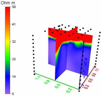
The ERT monitoring as described in Table 1 produced two clear results:

20

1. The initial conditions (11:00 of 2 October, before irrigation starts) around the tree

show a very clear difference in electrical resistivity in the top 40 cm of soil with

re-spect to the rest of the volume (Fig. 5). Specifically, the resistivity of the top layer

ranges around 40–50Ωm−1, while the lower part of the profile is about one order

of magnitude more conductive (about 5Ωm−1). As no apparent lithological diff

er-25

(11)

HESSD

11, 13353–13384, 2014

G. Cassiani et al.

Title Page

Tables Figures

◭ ◮

Back Close

Full Screen / Esc

Discussion

P

a

per

|

Discussion

P

a

per

|

Discussion

P

a

per

|

Discussion

P

a

per

|

this difference to a marked difference in soil moisture content. This was confirmed

by all following evidence (see below).

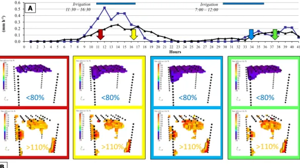
2. The resistivity changes as a function of time, during the two irrigation periods, during the night interval, and afterwards, all show essentially the same pattern, with relatively small (but still clearly measureable) changes (Fig. 6). Two zone are

5

identifiable: (a) a shallow zone (top 10–20 cm) where resistivity decreases with respect to the initial condition, and (b) a deeper zone (20–40 cm) where resistivity increases.

Qualitatively, both pieces of evidence can be easily explained in terms of water dynam-ics governed by precipitation, irrigation and root water uptake. Specifically, the

shal-10

lower high resistivity zone in Fig. 5 can be correlated to a dry region where root water

uptake manages to keep soil moisture content to minimal values, as an effect of the

en-tire summer strong transpiration drive. The dynamics in Fig. 6, albeit small compared to the initial root uptake signal in Fig. 5, still confirm that the top 40 cm is house to a strong root activity, to the point that irrigation cannot raise electrical conductivity of the

shal-15

low zone (10–20 cm) by no more than some 20 %, and the roots manage to make the soil even drier (with a resistivity increase by some 10 %) in the 20–40 cm depth layer (Fig. 6). Note that, in general, resistivity changes of the type here observed cannot be uniquely associated to soil moisture content changes, as pore water conductivity may play a key role (e.g. Boaga et al., 2013; Ursino et al., 2014). However, in the particular

20

case at hand, care was taken to analyze the electrical conductivity of both the water used for irrigation and the pore water, purposely extracted at about 50 cm depth. Both

waters showed an electrical conductivity value in the range of 1300 µ S cm−1_{(thus fairly}

high, fact that explains the overall small soil resistivity observed at the site). Therefore

in this particular case we can exclude pore water conductivity effects in the observed

25

(12)

HESSD

11, 13353–13384, 2014

G. Cassiani et al.

Title Page

Tables Figures

◭ ◮

Back Close

Full Screen / Esc

Discussion

P

a

per

|

Discussion

P

a

per

|

Discussion

P

a

per

|

Discussion

P

a

per

|

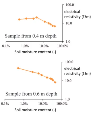
The qualitative evidence above is, however, not very surprising and not particularly informative: the root activity dries the soil, this is not a discovery. Things become more interesting if we can translate the ERT data into quantitative estimates of soil moisture content, and if we can use these data to calibrate hydrological models of the root zone. To this end, we tested Bulgherano soil samples in the laboratory to obtain a suitable

5

constitutive relationship linking moisture content and resistivity, given the know pore water conductivity that was reproduced for the water used in the laboratory. Figure 7

shows two examples of experimental results on samples from two different depths.

Note how in a wide range of soil moisture content (roughly from 5 % to saturation) the two curves in Fig. 7 lie practically on top of each other. The same applies for all tested

10

samples. Note also that, even though some samples show the effect of the conductivity

of the solid phase (through its clay fraction) at small saturation (see sample from 0.4 m

in Fig. 7) still the effect is small as it appears only at soil moisture smaller than 3–4 %.

Therefore we deemed unnecessary to resort to constitutive laws that represent this

solid phase effect, such as Waxman and Smits (1968) that has been used for similar

15

purposes elsewhere (e.g. Cassiani et al., 2012) and we adopted a simpler Archie’s (1942) formulation. Consequently we translated resistivity into moisture content using the following relationship calibrated on the laboratory data, using a water having the above mentioned electrical conductivity:

θ=4.703

ρ1.12 (1)

20

whereθis volumetric soil moisture content (dimensionless) andρis electrical resistivity

(in Ωm−1). The relationship (1) allows a direct translation of the 3-D resistivity

distri-bution to a corresponding distridistri-bution of volumetric soil moisture content. However, it has long been established that inverted geophysical data may bring with them enough distortion of the true physical parameter field (Day-Lewis et al., 2005) as to induce

25

(13)

HESSD

11, 13353–13384, 2014

G. Cassiani et al.

Title Page

Tables Figures

◭ ◮

Back Close

Full Screen / Esc

Discussion

P

a

per

|

Discussion

P

a

per

|

Discussion

P

a

per

|

Discussion

P

a

per

|

problems, particular when the use of data is expected to shift from a qualitative interpre-tation to a quantitative use in terms of data assimilation into hydrological models. For this reason, coupled vs. uncoupled approaches have been proposed and discussed (Hinnell et al., 2010) even though their superiority seems to depend on the specific problem, as the information content of data even in a tradition, inverted approach may

5

be sufficient (Camporese et al., 2011, 2014). Indeed, the geometry we are considering

here is very effective to reconstruct the mass balance of irrigated water, as this comes

as a quasi-one dimensional infiltration front from the top, where in addition electrodes are located. The geometry is similar to the one used, e.g. Koestel et al. (2008) where mass balance was verified by comparison against very detailed TDR data collected in

10

a lysimeter. In spite of these considerations, we decided to still limit ourselves to analyz-ing the data variation principally as a function of depth, lumpanalyz-ing the data horizontally by averaging estimated moisture content along two-dimensional horizontal planes. Note that the dataset may lend itself to more complex analyses such as the one proposed by Manoli et al. (2014), especially if used in the context of a formal Data Assimilation,

15

but we felt that one such an endeavor would exceed the scope of the current paper and deserves an ad-hoc space. Note also that the ERT field evidence both in terms of background (Fig. 5) and time-lapse evolution (Fig. 6) of moisture content confirm the hypothesis that, within the control volume, the distribution of water in the soil is largely one-dimensional as a function of depth.

20

The data, once condensed in this manner, lend themselves more easily to a compar-ison with the results of infiltration modeling. We implemented a one-dimensional finite element model based on a Richards’ equation solver (Lin et al., 1997), simulating the central square meter of the ERT monitored control volume, down to a total depth of 2 m (much below the depth of the ERT boreholes), where we assumed that the water table

25

is located. We therefore considered only the central part of the ERT-controlled volume

(1 m×1 m) thus excluding the regions too close to the boreholes that, even though

(14)

HESSD

11, 13353–13384, 2014

G. Cassiani et al.

Title Page

Tables Figures

◭ ◮

Back Close

Full Screen / Esc

Discussion

P

a

per

|

Discussion

P

a

per

|

Discussion

P

a

per

|

Discussion

P

a

per

|

by the drilling and installing operations. Correspondingly we averaged horizontally the ERT data only in this central region.

A very fine vertical discretization (0.01 m) and time stepping (0.01 h) ensures solu-tion stability. The porous medium is homogeneous along the column and parameter-ized according to the Van Genuchten (1980) model. The relevant parameters had been

5

derived independently from laboratory and field measurements, the latter particularly relevant for the definition of a reliable in situ saturated hydraulic conductivity estimate.

The parameters used for the simulations are: residual moisture contentθr=0.0,

poros-ityθs=0.54,α=0.12 m−

1

,n=1.6, saturated hydraulic conductivityKs=0.002 m h−

1

. The remaining elements of the predictive modeling exercise are initial and

bound-10

ary conditions. As we focused primarily our attention on reproducing the state of the system at background conditions, we set the start of the simulation at the beginning of the year (1 January 2013), and we assumed for that time a condition drained to equilibrium. Given the van Genuchten parameters we used and the depth of the wa-ter table, this corresponds to a fairly wet initial condition. We verified a poswa-teriori that

15

moving the initial time back of one or more years did not alter the predicted results at

the date of interest (3 October 2013). The dynamics during the year are sufficient to

bring the system to the real, much drier condition in October. The forcing conditions on the system are all known: (a) irrigation is recorded, and only one dripper pertains to the considered square meter, (b) precipitation is measured, (c) sap flow is measured.

20

Direct evaporation from the square meter of soil around the stem is neglected, consid-ering the dense canopy cover and the consequent limited radiation received. Only one degree of freedom is left to be calibrated, i.e. the volume from which the roots uptake water. Thickness of the active root zone was estimated from the time-lapse observa-tions (Fig. 6), and fixed to the top 0.4 m after checking that limiting the root uptake to the

25

(15)

HESSD

11, 13353–13384, 2014

G. Cassiani et al.

Title Page

Tables Figures

◭ ◮

Back Close

Full Screen / Esc

Discussion

P

a

per

|

Discussion

P

a

per

|

Discussion

P

a

per

|

Discussion

P

a

per

|

Figure 8 shows the results of the calibration exercise. It is apparent that the total areal extent of the root uptake zone has a dramatic impact on the predicted moisture content profiles, as it scales the amount of water subtracted from the monitored square meter

considered in the calibration. Even relatively small changes (±15 %) of the root uptake

area produce very different soil moisture profiles. The value that allows a good match

5

of the observed profile is 1.75 m2, while for areas equal to 1.5 and 2 m2 the match is

already unsatisfactory, leading respectively to underestimation and overestimation of the moisture content in the profile.

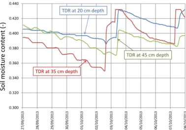
Another important fact that is apparent from Fig. 8 is that the estimated soil moisture

in the shallow zone (roughly down to 0.4 m) is very small as an effect of root water

up-10

take. However this dry zone must have a limited areal extent (1.75 m2, corresponding

to a radius of about 0.75 m from the stem of the tree). Indeed this is indirectly confirmed by the soil moisture evolution measured by TDR. Figure 9 shows the TDR data from three probes located about 1.5 m from the monitored tree (thus outside our estimated root uptake zone). The signal coming from the irrigation experiment of 2 October 2013

15

is very apparent with an increase in moisture content of all three probes, located at

different depths. Note that before this experiment the system had been left without

irri-gation for about two weeks. The corresponding effect on the TDR data is apparent: all

three probes show a decline of moisture content during the day, with pauses overnight. The decline is more pronounced in the 0.35 m TDR probe, that lies at a depth we

esti-20

mated to be nearly at the bottom of the RWU zone, and less pronounced above (0.2 m) and below (0.45 m). Note also that the TDR probes are close to another dripper, lying outside of the ERT controlled volume (the drippers are spaced 1 m along the orange trees line, with the trees about 4 m from each other) thus they reflect directly the infiltra-tion from that dripper. However, at all three depths the moisture content is much higher

25

than measured in the ERT-controlled block closer to the tree. This can be explained with the fact that in that region the root uptake is minimal or totally absent, while the

(16)

HESSD

11, 13353–13384, 2014

G. Cassiani et al.

Title Page

Tables Figures

◭ ◮

Back Close

Full Screen / Esc

Discussion

P

a

per

|

Discussion

P

a

per

|

Discussion

P

a

per

|

Discussion

P

a

per

|

root zone by lateral movement induced by the very strong capillary forces exerted by the dry fine grained soil in the active root zone closer to the tree.

5 Conclusions

Near surface geophysics is strongly affected by both static and dynamic soil/subsoil

characteristics. This fact, if properly recognized, is potentially full of information on the

5

soil/subsoil structure and behaviour. The information is maximized if geophysical data are collected in time-lapse mode. In the case of interactions with vegetation, its role should be properly modelled, and such models can be constrained by means (also) of geophysical data. This case study demonstrates that 3-D ERT is capable of char-acterizing the pathways of water distribution, and provides spatial information on root

10

zone suction regions. The integration of modeling and data has proven, once again, a key component of this type of hydro-geophysical studies, allowing us to draw quanti-tative results of practical interest. In this case we had available a wealth of quantiquanti-tative information about transpiration and soil moisture content that allowed the definition of

the volume of soil affected by the RWU activity. This has obvious consequences for

15

the possible improvement of irrigation strategies, as it is apparent how the monitored orange tree essentially drives water from 1 to 2 drippers out of the 4 total that should pertain to its area in the plantation. This means that it is very likely that half of the irrigated water is indeed lost to deeper layers and brings no contribution to the plants. More advanced uses of this type of data are now considered, especially linking soil

20

(17)

HESSD

11, 13353–13384, 2014

G. Cassiani et al.

Title Page

Tables Figures

◭ ◮

Back Close

Full Screen / Esc

Discussion

P

a

per

|

Discussion

P

a

per

|

Discussion

P

a

per

|

Discussion

P

a

per

|

Acknowledgements. We wish to acknowledge support from the EU FP7 project GLOBAQUA

(“Managing the effects of multiple stressors on aquatic ecosystems under water scarcity”) and the MIUR PRIN project 2010JHF437 “Innovative methods for water resources management under hydro-climatic uncertainty scenarios”. We also wish to thank the Agro-meteorological Service of the Sicilian Region for supporting field campaigns.

5

References

Aiello, R., Bagarello, V., Barbagallo, S., Consoli, S. Di Prima, S., Giordano, G., and Iovino, M.: An assessment of the Beerkan method for determining the hydraulic properties of a sandy loam soil, Geoderma, 235, 300–307, 2014.

al Hagrey, S. A.: Geophysical imaging of root-zone, trunk, and moisture heterogeneity, J. Exp.

10

Bot., 58, 839–854, 2007.

al Hagrey, S. A. and Petersen, T.: Numerical and experimental mapping of small root zones using optimized surface and borehole resistivity tomography, Geophysics, 76, G25–G35, doi:10.1190/1.3545067, 2011.

Allred, B., Daniels, J. J., and Reza Ehsani, M.: Handbook of Agricultural Geophysics, CRC

15

Press, University of Florida, Gainesville, FL, USA, 432 pp., 2008.

Archie, G. E.: The electrical resistivity log as an aid in determining some reservoir characteris-tics, T. ISS AIME, 146, 54–67, 1942.

Binley, A.: http://www.es.lancs.ac.uk/people/amb/Freeware/freeware.htm, last access: Au-gust 2014.

20

Binley, A., Ramirez, A., and Daily, W.: Regularised image reconstruction of noisy electrical re-sistance tomography data. in: Process Tomography, Proceedings of the 4th Workshop of the European Concerted Action on Process Tomography, 6–8 April 1995, edited by: Beck, M. S., Hoyle, B. S., Morris, M. A., Waterfall, R. C., and Williams, R. A., Bergen, 401–410, 1995. Binley, A. M. and Kemna, A.: DC resistivity and induced polarization methods, in:

Hydro-25

geophysics, edited by: Rubin, Y. and Hubbard, S. S., Water Sci. Technol. Library, Ser. 50. Springer, New York, 129–156, 2005.

(18)

HESSD

11, 13353–13384, 2014

G. Cassiani et al.

Title Page

Tables Figures

◭ ◮

Back Close

Full Screen / Esc

Discussion

P

a

per

|

Discussion

P

a

per

|

Discussion

P

a

per

|

Discussion

P

a

per

|

Binley, A. M., Cassiani, G. and Deiana, R.: Hydrogeophysics – opportunities and challenges, B. Geofis. Teor. Appl., 51, 267–284, 2011.

Boaga, J., Rossi, M., and Cassiani, G.: Monitoring soil–plant interactions in an apple orchard using 3-D electrical resistivity tomography, Conference on Four Decades of Progress in Mon-itoring and Modeling of Processes in the soil–plant-Atmosphere System: Applications and

5

Challenges, Series: Procedia Environmental Sciences, 19–21 June 2013, Naples, 394–402, 2013.

Boaga, J., D’Alpaos, A., Cassiani, G., Marani, M., and Putti, M.: Plant-soil interactions in salt-marsh environments: experimental evidence from electrical resistivity tomography (ERT) in the Venice lagoon, Geophys. Res. Lett., 41, 6160–6166, 2014.

10

Camporese, M., Salandin, P., Cassiani, G., and Deiana, R.: Impact of ERT data inversion un-certainty on the assessment of local hydraulic properties from tracer test experiments, Water Resour. Res., 47, W12508, doi:10.1029/2011WR010528, 2011.

Camporese, M., Cassiani, G., Deiana, R., Salandin, P., and Binley, A. M.: Comparing coupled and uncoupled hydrogeophysical inversions using ensemble Kalman filter assimilation of

15

ERT-monitored tracer test data, Water Resour. Res., submitted, 2014.

Cassiani, G., Bruno, V., Villa, A., Fusi, N., and Binley, A. M.: A saline trace test monitored via time-lapse surface electrical resistivity tomography, J. Appl. Geophys., 59, 244–259, 2006. Cassiani, G., Godio, A., Stocco, S., Villa, A., Deiana, R., Frattini, P., and Rossi, M.: Monitoring

the hydrologic behaviour of steep slopes via time-lapse electrical resistivity tomography, Near

20

Surf. Geophys., 7, 475–486, doi:10.3997/1873-0604.2009013, 2009.

Cassiani, G., Ursino, N., Deiana, R., Vignoli, G., Boaga, J., Rossi, M., Perri, M. T., Blaschek, M., Duttmann, R., Meyer, S., Ludwig, R., Soddu, A., Dietrich, P., and Werban, U.: Non-invasive monitoring of soil static characteristics and dynamic states: a case study highlighting vege-tation effects, Vadose Zone J., 11, vzj2011.0195, doi:10.2136/vzj2006.0137, 2012.

25

Castellví, F., Consoli, S., and Papa, R.: Sensible heat flux estimates using two different methods based on Surface renewal analysis. A study case over an orange orchard in Sicily, Agr. Forest Meteorol., 152, 58–64, 2012.

Consoli, S. and Papa, R.: Corrected surface energy balance to measure and model the evap-otranspiration of irrigated orange orchards in semi-arid Mediterranean conditions, Irrigation

30

(19)

HESSD

11, 13353–13384, 2014

G. Cassiani et al.

Title Page

Tables Figures

◭ ◮

Back Close

Full Screen / Esc

Discussion

P

a

per

|

Discussion

P

a

per

|

Discussion

P

a

per

|

Discussion

P

a

per

|

Couvreur, V., Vanderborght, J., and Javaux, M.: A simple three-dimensional macroscopic root water uptake model based on the hydraulic architecture approach, Hydrol. Earth Syst. Sci., 16, 2957–2971, doi:10.5194/hess-16-2957-2012, 2012.

Daily, W., Ramirez, A., LaBrecque, D., and Nitao, J.: Electrical resistivity tomography of vadose zone movement, Water Resour. Res., 28, 1429–1442, 1992.

5

Day-Lewis, F. D., Singha, K., and Binley, A. M.: Applying petrophysical models to radar travel time and electrical resistivity tomograms: resolution-dependent limitations, J. Geophys. Res.-Sol. Ea., 110, B08206, doi:10.1029/2004JB003569, 2005.

Doussan, C., Pierret, A., Garrigues, E., and Pagès, L.: Water uptake by plant roots: II – mod-elling of water transfer in thesoil root-system with explicit account of flow within the root

10

system – comparison with experiments, Plant Soil, 283, 99–117, doi:10.1007/s11104-004-7904-z, 2006.

Feddes, R. A., Hoff, H., Bruen, M., Dawson, T., de Rosnay, P., Dirmeyer, P., Jackson, R. B., Kabat, P., Kleidon, A., Lilly, A., and Pitman, A. J.: Modelling root water uptake in hydrological and climate models, B. Am. Meteorol. Soc., 82, 2797–2809, 2001.

15

Gong, D., Shaozhong, K., Zhang, L., Taisheng, D., and Limin, Y.: A two-dimensional model of root water uptake for single apple trees and its verification with sap flow and soil water content measurements, Agr. Water Manage., 83, 119–129, 2006.

Green, S. R., Vogeler, I., Clothier, B. E., Mills, T. M., and van den Dijssel, C.: Modelling water uptake by a mature apple tree, Aust. J. Soil Res., 41, 365–380, 2003a.

20

Green, S. R., Clothier, B., and Jardine, B.: Theory and practical application of heat pulse to measure sap flow, Agron. J., 95, 1371, doi:10.2134/agronj2003.1371, 2003b.

Hinnell, A. C., Ferré, T. P. A., Vrugt, J. A., Huisman, J. A., Moysey, S., Rings, J., and Kowalsky, M. B.: Improved extraction of hydrologic information from geophysical data through coupled hydrogeophysical inversion, Water Resour. Res., 46, W00D40,

25

doi:10.1029/2008WR007060, 2010.

Jarvis, N. J.: A simple empirical-model of root water-uptake, J. Hydrol., 107, 57–72, doi:10.1016/0022-1694(89)90050-4, 1989.

Javaux, M., Schroder, T., Vanderborght, J., and Vereecken, H.: Use of a three-dimensional detailed modeling approach for predicting root water uptake, Vadose Zone J., 7, 1079–1088,

30

(20)

HESSD

11, 13353–13384, 2014

G. Cassiani et al.

Title Page

Tables Figures

◭ ◮

Back Close

Full Screen / Esc

Discussion

P

a

per

|

Discussion

P

a

per

|

Discussion

P

a

per

|

Discussion

P

a

per

|

Jayawickreme, H., Van Dam, R., and Hyndman, D. W.: Subsurface imaging of vegeta-tion, climate, and root-zone moisture interactions, Geophys. Res. Lett., 35, L18404, doi:10.1029/2008GL034690, 2008.

Jones, H. G. and Tardieu, F.: Modelling water relations of horticultural crops: a review, Sci. Hortic-Amsterdam, 74, 21–46, 1998.

5

Kemna, A., Vanderborght, J., Kulessa, B., and Vereecken, H.: Imaging and characterisation of subsurface solute transport using electrical resistivity tomography ERT and equivalent transport models, J. Hydrol., 267, 125–146, 2002.

Koestel, J., Kemna, A., Javaux, M., Binley, A., and Vereecken, H.: Quantitative imaging of solute transport in an unsaturated and undisturbed soil monolith with 3-D ERT and TDR, Water

10

Resour. Res., 44, W12411, doi:10.1029/2007WR006755, 2008.

Lin, H. J., Richards, D. R., Talbot, C. A., Yeh, G.-T., Cheng, J., and Cheng, H.: FEMWATER: A Three-Dimensional Finite Element Computer Model For Simulating Density-Dependent Flow and Transport in Variably Saturated Media, US Army Corps of Engineers and Pennsylvania State University Technical Report CHL-97-12, Vicksburg, MS, 1997.

15

Manoli, G., Bonetti, S., Domec, J. C., Putti, M., Katul, G., and Marani, M.: Tree root sys-tems competing for soil moisture in a 3-D soil–plant model, Adv. Water Resour., 66, 32–42, doi:10.1016/j.advwatres.2014.01.006, 2014.

Mauder, M. and Foken, T.: Documentation and instruction manual of the eddy covariance software package TK2, Abt. Mikrometeorologie, Arbeitsergebnisse, Universität Bayreuth,

20

Bayreuth, 26–44, 2004.

Mauder, M., Oncley, S. P., Vogt, R., Weidinger, T., Ribeiro, L., Bernhofer, C., Foken, T., Kosiek, W., De Bruin, H. A. R., and Liu, H.: The energy balance experiment EBEX-2000, Part II. Intercomparison of eddy-covariance sensors and post-field data processing meth-ods, Bound.-Lay. Meteorol., 123, 29–54, doi:10.1007/s10546-006-9139-4, 2007.

25

Moncrieff, J. B., Clement, R., Finnigan, J. J., and Meyers, T.: Averaging and de-trending, in: Handbook of Micrometeorology, edited by: Lee, X., Massman, W., and Law, B., Kluwer Acad. Publ., the Netherlands, 7–31, 2004.

Monego, M., Cassiani, G., Deiana, R., Putti, M., Passadore, G., and Altissimo, L.: Tracer test in a shallow heterogeneous aquifer monitored via time-lapse surface ERT, Geophysics, 75,

30

(21)

HESSD

11, 13353–13384, 2014

G. Cassiani et al.

Title Page

Tables Figures

◭ ◮

Back Close

Full Screen / Esc

Discussion

P

a

per

|

Discussion

P

a

per

|

Discussion

P

a

per

|

Discussion

P

a

per

|

Motisi, A., Consoli, S., Rossi, F., Minacapilli, M., Cammalleri, C., Papa, R., Rallo, G., and D’urso G.: Eddy covariance and sap flow measurement of energy and mass exchange of woody crops in a Mediterranean environment, Acta Hortic., 951, 121–127, 2012.

Musters, P. A. D. and Bouten, W.: A method for identifying optimum strategies of measuring soil water contents for calibrating a root water uptake model, J. Hydrol., 227, 273–286, 2000.

5

Parasnis, D. S.: Mining Geophysics, Elsevier Scientific Pub. Co., Amsterdam, New York, 395 pp., 1973.

Perri, M. T., Cassiani, G., Gervasio, I., Deiana, R., and Binley, A. M.: A saline tracer test mon-itored via both surface and cross-borehole electrical resistivity tomography: comparison of time-lapse results, J. Appl. Geophys., 79, 6–16, doi:10.1016/j.jappgeo.2011.12.011, 2012.

10

Raats, P. A. C.: Uptake of water from soils by plant roots, Transp. Porous Med., 68, 5–28, 2007. Rubin, Y. and Hubbard, S. S. (Eds.): Hydrogeophysics, Springer, Dordrecht, 523 pp., 2005. Schneider, C. L., Attinger, S., Delfs, J.-O., and Hildebrandt, A.: Implementing small scale

pro-cesses at the soil–plant interface – the role of root architectures for calculating root water uptake profiles, Hydrol. Earth Syst. Sci., 14, 279–289, doi:10.5194/hess-14-279-2010, 2010.

15

Sheets, K. R. and Hendrickx, J. M. H.:: Non invasive soil water content measurement using electromagnetic induction, Water Resour. Res., 31, 2401–2409, 1995.

Singha, K. and Gorelick, S. M.: Saline tracer visualized with three dimensional electrical re-sistivity tomography: field-scale spatial moment analysis, Water Resour. Res., 41, W05023, doi:10.1029/2004WR003460, 2005.

20

Ursino, N., Cassiani, G., Deiana, R., Vignoli, G., and Boaga, J.: Measuring and modeling water-related soil–vegetation feedbacks in a fallow plot, Hydrol. Earth Syst. Sci., 18, 1105–1118, doi:10.5194/hess-18-1105-2014, 2014.

Van Genuchten, M. T.: A closed form equation for predicting the hydraulic conductivity of un-saturated soils, Soil Sci. Soc. Am. J., 44, 892–898, 1980.

25

Vereecken, H., Binley, A., Cassiani, G., Kharkhordin, I., Revil, A., and Titov, K.: Applied Hydro-geophysics, Springer-Verlag, Berlin, 2006.

Waxman, M. H. and Smits, L. J. M.: Electrical conductivities in oil-bearing shaly sands, Soc. Petrol. Eng. J., 8, 107–122, 1968.

Weill, S., Altissimo, M., Cassiani, G., Deiana, R., Marani, M., and Putti, M.: Saturated area

30

(22)

HESSD

11, 13353–13384, 2014

G. Cassiani et al.

Title Page

Tables Figures

◭ ◮

Back Close

Full Screen / Esc

Discussion

P

a

per

|

Discussion

P

a

per

|

Discussion

P

a

per

|

Discussion

P

a

per

|

Werban, U., al Hagrey, S. A., and Rabbel, W.: Monitoring of root-zone water content in the laboratory by 2-D geoelectrical tomography, J. Plant Nutr. Soil Sc., 171, 927–935, doi:10.10027jpln.200700145, 2008.

Wilson, K. B., Goldstein, A. H., and Falge, E.: Energy balance closure at FLUXNET sites, Agr. Forest Meteorol., 113, 223–243, 2002.

(23)

HESSD

11, 13353–13384, 2014

G. Cassiani et al.

Title Page

Tables Figures

◭ ◮

Back Close

Full Screen / Esc

Discussion

P

a

per

|

Discussion

P

a

per

|

Discussion

P

a

per

|

Discussion

P

a

per

|

Table 1.Times of acquisitions and irrigation schedule.

Acquisition Starting Ending Irrigation Date

# time time schedule

0 (background) 10:40 11:00 11:30 to 16:30 2 Oct 2013 1 12:00 12:20 4 L h−1

from 2 13:00 13:20 each dripper

3 14:15 14:35

4 15:00 15:20

5 16:00 16:20

6 17:00 17:20

7 10:15 10:35 07:00 to 12:00 3 Oct 2013 8 11:05 11:25 4 L h−1

from 9 12:00 12:20 each dripper

10 13:00 13:20

11 14:00 14:20

12 15:00 15:20

(24)

HESSD

11, 13353–13384, 2014

G. Cassiani et al.

Title Page

Tables Figures

◭ ◮

Back Close

Full Screen / Esc

Discussion

P

a

per

|

Discussion

P

a

per

|

Discussion

P

a

per

|

Discussion

P

a

per

|

Figure 1.Bulgherano experimental site: the Eddy Covariance (EC) tower and a Heat Pulse

(25)

HESSD

11, 13353–13384, 2014

G. Cassiani et al.

Title Page

Tables Figures

◭ ◮

Back Close

Full Screen / Esc

Discussion

P

a

per

|

Discussion

P

a

per

|

Discussion

P

a

per

|

Discussion

P

a

per

|

Figure 2.Energy Balance closure at the Bulgherano experimental site.

(26)

HESSD

11, 13353–13384, 2014

G. Cassiani et al.

Title Page

Tables Figures

◭ ◮

Back Close

Full Screen / Esc

Discussion

P

a

per

|

Discussion

P

a

per

|

Discussion

P

a

per

|

Discussion

P

a

per

|

Figure 3.3-D ERT apparatus installed around one orange tree. The system is composed of

four micro-boreholes carrying 12 electrodes each (see inset) and 24 surface electrodes – see text and Fig. 4 for geometry details.

(27)

HESSD

11, 13353–13384, 2014

G. Cassiani et al.

Title Page

Tables Figures

◭ ◮

Back Close

Full Screen / Esc

Discussion

P

a

per

|

Discussion

P

a

per

|

Discussion

P

a

per

|

Discussion

P

a

per

|

Figure 4.Electrode geometry around the orange tree and 3-D mesh used for ERT inversion.

(28)

HESSD

11, 13353–13384, 2014

G. Cassiani et al.

Title Page

Tables Figures

◭ ◮

Back Close

Full Screen / Esc

Discussion

P

a

per

|

Discussion

P

a

per

|

Discussion

P

a

per

|

Discussion

P

a

per

|

Figure 5. Cross-sections of the ERT cube corresponding to the background acquisition of

(29)

HESSD

11, 13353–13384, 2014

G. Cassiani et al.

Title Page

Tables Figures

◭ ◮

Back Close

Full Screen / Esc

Discussion

P

a

per

|

Discussion

P

a

per

|

Discussion

P

a

per

|

Discussion

P

a

per

|

0.0 0.1 0.2 0.3 0.4 0.5 0.6

0 1 2 3 4 5 6 7 8 9 10 11 12 13 14 15 16 17 18 19 20 21 22 23 24 25 26 27 28 29 30 31 32 33 34 35 36 37 38 39 40 41

(mm h

-1)

Hours

Irrigation 7:00 – 12:00 Irrigation

11:30 – 16:30

A

B

<80%

>110%

<80%

>110% >110%

<80% <80%

>110%

Figure 6. (a)Time series of sap flow (black line) and EC-derived total evapotranspiration (blue

lines), both normalized in mm assuming an area of 20 m2pertaining to the orange tree moni-tored with ERT. Time is given in hours from midnight of 2 October. The two irrigation periods are shown by the blue bars.(b)3-D ERT images of resistivity change with respect to background at four selected time instants shown by the arrows in(a); the volumes corresponding to increase and decrease of resistivity above and below certain thresholds (80 and 110 %) are shown in separate panels, for clarity.

(30)

HESSD

11, 13353–13384, 2014

G. Cassiani et al.

Title Page

Tables Figures

◭ ◮

Back Close

Full Screen / Esc

Discussion

P

a

per

|

Discussion

P

a

per

|

Discussion

P

a

per

|

Discussion

P

a

per

|

Soil moisture content (-)

electrical

resistivity (Ωm)

electrical

resistivity (Ωm)

Figure 7.Experimental relationships between resistivity and moisture content determined in

(31)

HESSD

11, 13353–13384, 2014

G. Cassiani et al.

Title Page

Tables Figures

◭ ◮

Back Close

Full Screen / Esc

Discussion

P

a

per

|

Discussion

P

a

per

|

Discussion

P

a

per

|

Discussion

P

a

per

|

0 0.2 0.4 0.6

soil moisture content (-) -2

-1.6 -1.2 -0.8 -0.4 0

d

e

p

th

b

e

lo

w

g

ro

u

n

d

(

m

)

real data: 12:00 noon October 2, 2013 initial conditions (1/1/2013)

1.75 m2 1.50 m2 1.25 m2 2.00 m2

2.25 m2

Figure 8.Results of 1-D Richards’ equation simulations of the entire year 2013 till 3 October,

(32)

HESSD

11, 13353–13384, 2014

G. Cassiani et al.

Title Page Abstract Introduction Conclusions References Tables Figures ◭ ◮ ◭ ◮ Back Close

Full Screen / Esc

Printer-friendly Version Interactive Discussion Discussion P a per | Discussion P a per | Discussion P a per | Discussion P a per | 0.300 0.320 0.340 0.360 0.380 0.400 0.420 0.440 27/ 09/ 2013 28/ 09/ 2013 29/ 09/ 2013 30/ 09/ 2013 01/ 10/ 2013 02/ 10/ 2013 03/ 10/ 2013 04/ 10/ 2013 05/ 10/ 2013 06/ 10/ 2013 07/ 10/ 2013 08/ 10/ 2013 So il m o is tur e co nte nt (-)

TDR at 20 cm depth

TDR at 35 cm depth

TDR at 45 cm depth

Figure 9.Moisture content time series from three TDR probes located about 1.5 m from the