Copyright: Wyższa Szkoła Logistyki, Poznań, Polska
LogForum
> Scientific Journal of Logistics <
http://www.logforum.net p-ISSN 1895-2038
2015, 11 (1), 119-126
e-ISSN 1734-459X
STRATEGIC
VEHICLE
FLEET
MANAGEMENT
- THE COMPOSITION PROBLEM
Adam Redmer
Poznan University of Technology, Poznan, Poland
ABSTRACT. Background: Fleets constitute the most important production means in transportation. Their appropriate management is crucial for all companies having transportation duties. The paper is the second one of a series of three papers that the author dedicates to the strategic vehicle fleet management topic.
Material and methods: The paper discusses ways of building companies' fleets of vehicles. It means deciding on the number of vehicles in a fleet (the fleet sizing problem - FS) and types of vehicles in a fleet (the fleet composition problem - FC). The essence of both problems lies in balancing transportation supply and demand taking into account different demand types to be fulfilled and different vehicle types that can be put into a fleet. Vehicles, which can substitute each other while fulfilling different demand types. In the paper an original mathematical model (an optimization method) allowing for the FS/FC analysis is proposed.
Results: An application of the proposed optimization method in a real-life decision situation (the case study) within the Polish environment and the obtained solution are presented. The solution shows that there exist some best fitted (optimal) fleet size / composition matching company's transportation requirements. An optimal fleet size / composition allows for a significantly higher fleet utilization (10-15% higher) than any other, including random fleet structure. Moreover, any changes in the optimal fleet size / composition, even small ones, result in a lower utilization of vehicles (lower by a few percent).
Conclusions: The presented in this paper analysis, on the one hand, is consistent with a widespread opinion that the number of vehicle types in a fleet should be limited. In the other words it means that the versatility / interchangeability of vehicles is very important. On the other hand, the analysis proves that even small changes in a fleet size / fleet composition can result in an important changes of the fleet effectiveness (measured for example by the utilization ratio).
Key words: management, optimization, fleet, transport, sizing, composition.
"Is your fleet the right size?" - David Kirby
INTRODUCTION
The decision of how many vehicles keep in a company's fleet to fulfil varying with time transportation requirements is called a fleet sizing (FS) problem [Gould, 1969]. Whereas, in case of a fleet composition (FC) problem types of vehicles should be defined as well [Etezadi and Beasley, 1983].
of a month (phenomenon so-called "the third decade syndrome").
The demand can also be of different types according to specific features of loads, distances, routes or locations of destination points / customers, their orders and many others. For example resulting in:
− transportation of commodities that require or not special treatment (e.g. general freights v. dangerous goods, loose materials, temperature controlled environment shipments),
− transportation of heavy and/or oversized loads,
− local, regional, domestic or international shipments (short- and long-distance haulage),
− urban, suburban or rural deliveries,
− less than truck-load (LTL) or full truck-load (FTL) shipments.
The demand for transportation services can be defined by a number of kilometers, ton-kilometers, tones, cubic-meters, pallets, liters or any other measure of loads to be transported /transports to be done within a given time period.
As a result, different (universal, specialized or special) types of vehicles of different load capacity (small, light, medium, heavy or even very heavy trucks) are necessary to transport particular types of loads. However, the range of load types being within transportation capabilities of particular types of vehicles is limited. It depends on both, the interrelationship of vehicle and load features and vehicle maximum productivity that can be split among particular demand types.
All the mentioned above features of the demand (level and seasonal changes of particular demand types) can lead to an oversized fleet or to an unmet demand (transportation requirements not fulfilled by vehicles in a fleet), or even both at the same time. The unmet demand usually cannot be backordered and has to be outsourced or lost. Moreover, some long-term changes of the demand can force fleet size changes (increases or reductions).
There are also very important economic aspects of the FS/FC problems. In contrast to using outside transportation resources (buying transportation services in the market from common carriers), an in-house transportation solution results not only in variable, but, what is very important, in fixed costs as well. The fixed costs have to be bore even though particular vehicles in a fleet do not work (are not utilized) at a particular time period. These are the costs of unused resources - downtime, empty movements, and underutilized vehicles' loading capacity and/or productivity e.g. mileage (due to seasonal or other changes of the transportation demand). On the other hand, a company operating their own fleet of vehicles has to cover costs of all kilometers travelled (loaded and empty ones).
What can reduce level of the unmet demand or too high fixed costs and at the same time increase utilization ratio of an in-house fleet is the right interchangeability/versatility of vehicles in a fleet. The interchangeability /versatility means ability of particular vehicles to serve particular demand types.
THE METHOD FOR SOLVING
THE FC PROBLEM
and Bodin 1983, Golden, Assad, Levy and Gheysens 1984, Renaud and Boctor 2002] and metaheuristic ones [Yepes and Medina 2006, Osman and Salhi 1996, Gendreau, Laporte, Musaraganyi and Taillard 1999].
Majority of the FS/FC solution methods balances supply and demand for transportation services. They adjust supply of transportation capabilities of a fleet to the demand for transportation services to be delivered. The supply is defined by a number of vehicles in a fleet and their capacity (e.g. tonnage or the Gross Vehicle Weight Rating - GVWR) and productivity (e.g. a maximum annul mileage). When considering the FC problem different types of vehicles serving different types of transportation demand are taken into account as well. The general aim of balancing supply and demand is to fulfil all the demand while minimizing overall costs or maximizing utilization ratio of a fleet.
The general drawback of the mentioned above solution methods is that they do not take into account an interchangeability of vehicles when serving different types of transportation demand. Usually a necessary numbers of vehicles in a fleet to serve particular demand types are calculated separately. While in practice vehicles of particular types are utilized to fulfill interchangeably different demand types, with lower or higher effectiveness and under some limitations of course. When it is not taken into account it can result in an oversized fleet.
The question arises how to balance transportation supply and demand assuming that particular vehicle types can serve particular demand types interchangeably? What will be the distribution of vehicles' productivity between particular types of demand?
The point is to assess the most probable number of kilometers that vehicle of a given type will travel carrying loads (serving demand) of a given type. Let assume that a vehicle of a particular type, having the maximum productivity of 100 kilometers per given period of time / analysis, can serve for example three types of demand (1, 2 and 3) requiring the following number of kilometers
to be covered: 100, 200 and 300 per period of analysis (600 kilometers in total). The probability that the vehicle will be engaged in carrying loads of the type 3 (the demand 3) is three times higher than the probability of carrying loads of the type 1, since the overall workload to be done associated with the demand type 3 is 300 kilometers, whereas for the demand type 1 it is 100 kilometers only. Based on this assumption, the maximum productivity of the vehicle can be most probably divided between the three demand types as follows: 17 kilometers traveled carrying loads of type 1 (it comes from 100 kilometers multiplied by 1/6 that is 100 kilometers being the total quantity of kilometers associated with the demand type 1 divided by 600 kilometers being the total number of kilometers to be covered within the period of analysis), 33 kilometers traveled carrying loads of type 2, and the rest that is 50 kilometers traveled carrying loads of type 3. But if there in the fleet are too many vehicles that can serve, for example, demand number 3, let assume 10 vehicles of the same type as the analyzed one, it means that each one of them can travel 30 kilometers only when serving demand type 3 (300 kilometers divided by 10 vehicles), not 50! And they are underutilized.
As a result a generic formula for calculating the number of vehicles of particular types j (j = 1, 2, 3, …, J) in a fleet, the number that maximizes utilization ratio of a fleet and allows for fulfilling the whole transportation demand divided into I types (i = 1, 2, 3, …, I) can be written as follows:
( )
(
)
∑
∑
∑
∑
= = = = ⋅ ⋅ ⋅ ⋅ ⋅ = I i I i i i J j I i ij i i ij j j i j P P P zW P P zW l W P Min l K 1 1 1 1 , 1under the condition:
(
)
∑
∑
= =≥
⋅
I i i J j jj
l
P
W
where:
KP(lj) - average utilization ratio of a fleet
composed of vehicles of particular types j in the quantity of lj vehicles of particular
types j [-],
lj - number of vehicles of particular types j
in a fleet, including 0 that allows for fleet composition adjustments as well - DECISION VARIABLES [-],
Pi - demand for transportation services of
a type i per period of analysis; i = 1, 2, 3, …, I [kilometers - km, tones - t, ton-kilometers - tkm, pallets - p, m3, liters - l,
routes - r, …/… e.g. one year],
Wj - average, real productivity of one
vehicle of a type j per period of analysis, expressed in the same units of measurement as the demand [km, t, tkm, p, m3, l, r, …/…],
zWij - productivity range of particular vehicle
types j in relation to demand types i denoting what types of demand can serve given type of vehicles; zWij ∈ {0, 1} -
binary value or zWij ∈〈0, 1〉[-],
Min{…}- minimum value of elements of a set.
THE CASE STUDY – SOLVING
THE FC PROBLEM IN POLISH
CIRCUMSTANCES
Let's consider a domestic transportation company operating in Poland. The company exploiting a fleet composed of 14 types of vehicles and serving 5 types of transportation demand (carrying 5 types of loads).
As for the demand types i, there are the following ones:
− i = 1: long-haul - regular loads - an average number of customers per one route 3 - an average weight of a load per one route 18t - an average number of cargo units per one route 30 pallets - an average length of one route 715 km - the total annual number of kilometers 2 000 000,
− i = 2: short-haul - regular loads - an average number of customers per one route 3 - an average weight of a load per one route 13.5t - an average number of cargo units per one route 27 pallets - an average length of one route 235 km - the total annual number of kilometers 900 000,
− i = 3: short-haul - temperature controlled loads - an average number of customers per one route 4 - an average weight of a load per one route 12t - an average number of cargo units per one route 12 pallets - an average length of one route 270 km - the total annual number of kilometers 1 100 000,
− i = 4: urban distribution - regular loads - an average number of customers per one route 6 - an average weight of a load per one route 6t - an average number of cargo units per one route 12 pallets - an average length of one route 135 km - the total annual number of kilometers 800 000,
− i = 5: urban distribution - regular and temperature controlled loads - an average number of customers per one route 4 - an average weight of a load per one route 6t - an average number of cargo units per one route 8 pallets - an average length of one route 185 km - the total annual number of kilometers 700 000.
As for the vehicle types j, there are the following ones:
− j = 1, 2, 3 and 4: tractors with semi-trailers - full tilt (curtain sided) - load capacity of 20, 24 and 26 tones / 33 pallets - maximum annual mileage 50 to 80 000 km - emission standard EURO3, 4 and 5 - age 3 to 10 years,
− j = 5: trucks - closed body - load capacity of 6 tones / 12 pallets - maximum annual mileage 82 000 km - emission standard EURO5 - age 1 year,
− j = 6,7 and 8: trucks - full tilt - load capacity of 8 and 10 tones / 14 and 16 pallets - maximum annual mileage 42 to 71 000 km - emission standard EURO3 and 5 - age 4 to 12 years,
− j = 9 and 10: trucks - isolated - load capacity of 14 tones / 18 and 20 pallets - maximum annual mileage 66 to 79 000 km - emission standard EURO4 and 5 - age 3 to 6 years,
− j = 11: trucks - refrigerated - load capacity of 16 tones / 18 pallets - maximum annual mileage 55 000 km - emission standard EURO3 - age 8 years,
− j = 14: vans - isolated - load capacity of 2 tones / 4 pallets - maximum annual mileage 67 000 km - emission standard EURO5 - age 2 years.
An optimal fleet composition balancing described above transportation supply and demand has been constructed maximizing the average, weighted utilization ratio KP(lj)
(taking into account a maximum annual mileage) of vehicles in the fleet under the constraint that the numbers lj of vehicles of particular types j will be high enough to fully satisfy the transportation demand of all types i.
In the analysis the limited ability of particular vehicle types to serve particular demand types has been taken into account. In details the maximum annual mileage of vehicles of particular types has been divided between the 5 demand types taking into account the matching of vehicles (their load capacities) to particular demand types (an average weight of loads and number of cargo units per one route) - see Table 1. For example, tractors with semi-trailers - full tilt (the vehicle types j = 1, 2, 3 and 4), irrespectively of their load capacity (20, 24 or 26 tones / 33 pallets), are suitable to serve the long-haul - regular load shipments (the demand type i=1), characterized by an average weight of a load of 18t /30 pallets per one route being 715-kilometer long on average and, however, with the less efficiency, the short-haul - regular load shipments (the demand type i=2), characterized by an average weight of a load of 13.5t / 27 pallets per one route being 235-kilometer long on average. And, they are not suitable to serve the short-haul - temperature controlled load shipments and the urban distribution as well (the demand types i = 3, 4 and 5).
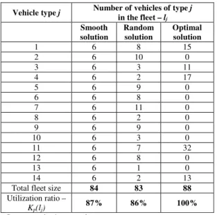
Using the proposed above mathematical model of the FS/FC problem, the above described data and a professional solver for the MS Excel the problem has been solved. The results are presented in Table 2.
Table 1. Ability of particular vehicle types to serve particular demand types Tabela 1. Możliwości obsługi danego rodzaju popytu
przez dany rodzaj pojazdu
Vehicle type j Demand type i
1 2 3 4 5
1 √ √
2 √ √
3 √ √
4 √ √
5 √ √
6 √ √ √
7 √ √
8 √ √ √ √
9 √ √ √ √
10 √ √ √ √
11 √ √
12 √
13 √
14 √ √
Source: author's research
Table 2. Selected solutions of the analyzed FC problem Tabela 2. Wybrane rozwiązania analizowanego
problemu kompozycji taboru
Vehicle type j Number of vehicles of type in the fleet – l j j
Smooth solution
Random solution
Optimal solution
1 6 8 15
2 6 10 0
3 6 3 11
4 6 2 17
5 6 9 0
6 6 8 0
7 6 11 0
8 6 2 0
9 6 9 0
10 6 3 0
11 6 7 32
12 6 8 0
13 6 1 0
14 6 2 13
Total fleet size 84 83 88
Utilization ratio –
Kp(lj) 87% 86% 100%
Source: author's research
economical. Of course the presented calculations are based on some assumptions and are significant simplification of the reality. However, one can expect that even though the real life utilization of a fleet will be lower than calculated, it will be lower for all the solutions (possible fleet compositions) to the same degree (a methodological error). So, the optimal solution should still denote a fleet composition assuring its best utilization.
It is also worthwhile to notice that based on the optimal solution the fleet is composed of 5 vehicle types only. The low number of vehicle types in a fleet, the easier to manage it.
The carried out sensitivity analysis revealed that any changes in the optimal composition of the analyzed fleet decreases its utilization. For example random changes of the number of vehicles of particular types by only 1 vehicle (increased number of vehicles of a one type, and at the same time decreased number of vehicles of another type, kipping the fleet size constant and the demand satisfaction constraint fulfilled) result in the decrease of the utilization ratio by 0.5%. If the number of the exchanged vehicles is 5 the utilization ratio decreases by 4.5%.
ACKNOWLEDGEMENTS
This scientific work was supported by the national funds for scientific research within the years 2010 and 2012 as a research project titled "The development of the quantitative strategic fleet management methodology" (the postdoctoral research project number N N509 570839 financed by the Ministry of Science and High Education in Poland).
CONCLUSIONS
The FS/FC decisions concerning types and number of vehicles in a fleet, as well as MoB decision problem, belong to the group of the strategic fleet management problems. These decisions as any other strategic ones concern relatively long-term planning and effects they cause are postponed in time. It means that to asses if the FS/FC decisions made were correct or wrong is possible after
a relatively long time (half a year to one year or even more). Moreover, such decisions are usually crucial and their results that are noticeable outside a company have an economical character (e.g. investments). That is the cause why it is very important to make this type of decisions not only intuitively, but first of all based on comprehensive and correct analysis. The presented in this paper analysis, on the one hand, is consistent with a widespread opinion that the number of vehicle types in a fleet should be limited (the lower, the better). It the other words it means that the versatility/ interchangeability of vehicles is very important. On the other hand, the analysis proves that even small changes in a fleet size/ fleet composition can result in an important changes of the fleet effectiveness (measured for example by the utilization ratio).
REFERENCES
Ball M.O., Golden B.L., Assad A.A., Bodin L.D., 1983, Planning for truck fleet size in the presence of common-carrier option, Decision Science, 14, 103-120. Beaujon G.J., Turnquist M.J., 1991, A model
for fleet sizing and vehicle allocation, Transportation Science, 25(1), 19-45. Dantzig G.B., Fulkerson D.R., 1954,
Minimizing the number of tankers to meet a fixed schedule, Naval Research Logistics Quarterly, 1, 217-222.
Du Y., Hall R., 1997, Fleet sizing and empty equipment redistribution for center-terminal transportation networks, Management Science, 43(2), 145-157.
Etezadi T., Beasley J.E., 1983, Vehicle fleet composition, Journal of Operational Research Society, 34, 87-91.
Fagerholt K., 1999, Optimal fleet design in a ship routing problem, International Transactions in Operational Research, 6, 453-464.
Golden B., Assad A.A., Levy L., Gheysens F.J., 1984, The fleet size and mix vehicle routing problem, Computers Operations Research, 11, 49-65.
Gould J., 1969, The size and composition of a road transport fleet, Operational Research Quarterly, 20, 81-92.
Hall N.G., Sriskandarajah C., Genesharajah T., 2001, Operational decisions in AGV-served flowshop loops: fleet sizing and decomposition, Annals of Operations Research, 107(1-4), 189-209.
Koo P-H., Jang J., Suh J., 2005, Estimation of part waiting time and fleet sizing in AGV systems, The International Journal of Flexible Manufacturing Systems, 16(3), 211-228.
Osman I.H., Salhi, S., 1996, Local search strategies for the vehicle fleet mix problem, in: Rayward-Smith, V.J., Osman, I.H., Reeves, C.R., and Smith, G.D. (eds.), Modern heuristic.
Parikh S.C., 1977, On a fleet sizing and allocation problem, Management Science, 23(9), 972-977.
Petering M.E.H., 2011, Decision support for yard capacity, fleet composition, truck substitutability, and scalability issues at seaport container terminals, Transportation Research Part E, 47, 85-103. Renaud J., Boctor F.F., 2002, A sweep-based algorithm for the fleet size and mix vehicle routing problem, European Journal of Operational Research, 140, 618-628. Wu P., Hartmann J.C., Wilson G.R., 2005,
An integrated model and solution approach for fleet sizing with heterogeneous assets, Transportation Science, 39, 87-103.
Yepes V., Medina J., 2006, Economic heuristic optimization for heterogeneous fleet VRPHESTW, Journal of Transportation Engineering, 132, 303-311.
Zak J., Redmer A., Sawicki P., 2008, Multiple objective optimization of the fleet sizing problem in the road freight transportation environment, Journal of Advanced Transportation, 42(4), 379-427.
STRATEGICZNE ZARZ
Ą
DZANIE TABOREM SAMOCHODOWYM
- PROBLEM KOMPOZYCJI
STRESZCZENIE. Wstęp: Floty pojazdów stanowią podstawowy środek produkcji w transporcie. Prawidłowe zarządzanie nimi jest zatem kluczowe dla wszystkich firm realizujących przewozy. Niniejszy artykuł jest drugim z serii trzech, jakie autor chce poświęcić tematyce strategicznego zarządzania taborem samochodowym.
Metody: W artykule omówiono sposoby kształtowania flot samochodowych przedsiębiorstw. To znaczy ustalenia liczby (problem liczebności - FS) i rodzajów pojazdów (problem kompozycji - FC) we flocie. Istota obu problemów leży w równoważeniu podaży i popytu na przewozy z uwzględnieniem różnych rodzajów popytu, jakie trzeba zaspokoić, oraz różnych rodzajów pojazdów, jakie mogą znaleźć się we flocie wraz z wzajemną zastępowalnością owych pojazdów przy zaspokajaniu poszczególnych rodzajów popytu. W artykule zaproponowano autorską, matematyczną metodę
(model optymalizacyjny) pozwalającą na prowadzenie analiz typu FS/FC.
Rezultaty: W artykule zaprezentowano zastosowanie opracowanej metody na rzeczywistym przykładzie problemu decyzyjnego w warunkach polskich oraz uzyskane rezultaty. Rezultaty te pokazały, że istnieje pewne, najlepsze (optymalne) dopasowanie struktury floty do potrzeb przewozowych. Rozwiązanie pozwalające na wykorzystanie taboru w stopniu istotnie wyższym (10-15%), niż w przypadku innych, w tym losowych, rozwiązań. A zmiana owego optymalnego rozwiązania, nawet w niewielkim stopniu, powoduje pogorszenie wykorzystania taboru o kilka procent. Wnioski: Prezentowana w pracy analiza jest z jednej strony zgodna popularną opinią, iż ilość typów samochodów we flocie powinna być ograniczona. Oznacza to, że uniwersalność i możliwość zmian w liczbie samochodów ma bardzo duże znaczenie. Z drugiej strony, prezentowana analiza potwierdza stwierdzenie, że nawet małe zmiany w wielkości floty i jej składzie mogą powodować istotne zmiany efektywności całej floty (mierzone na przykład, jako procent użytkowania).
STRATEGISCHES FAHRZEUGFLOTTENMANAGEMENT - DAS
PROBLEM DER FLOTTENZUSAMMENSETZUNG
ZUSAMMENFASSUNG.Einleitung: Fahrzeugflotten und Fuhrparks stellen das Rückgrat der Verkehrsproduktion dar. Ein angemessenes Flottenmanagement ist für alle Gesellschaften und Firmen mit Transportaufgaben von großem Belang. Der vorliegende Artikel ist der zweite von dreien, die der Autor dem strategischen Fahrzeugflottenmanagement widmet. Methoden: Dieser Artikel beschreibt Möglichkeiten für Unternehmen ihre Fahrzeugflotte zusammenzusetzen. Dies beinhaltet sowohl die Beantwortung der Frage nach der Flottengröße (the fleet sizing problem - FS) und der Zusammensetzung der Fahrzeugflotte (the fleet composition problem - FC). Der Kern beider Probleme liegt dabei darin, Angebot und Nachfrage nach Transportdienstleistungen so auszubalancieren, dass der Typ der Fahrzeugnachfrage auf Basis verschiedener Fahrzeugtypen einer Flotten bedient werden kann. Verschiedene Fahrzeugtypen können dabei substituierend eingesetzt werden. Im vorliegenden Artikel wird dabei ein ursprünglich mathematisches Modell (Optimierungsmethode) zur FS/FC-Analyse vorgestellt.
Ergebnisse: Es werden die Umsetzung und Ergebnisse einer Anwendung der vorgestellten Optimierungsmethode im Rahmen eines Feldversuchs in Polen präsentiert. Die Lösung zeigt, dass es eine optimale Flottengröße und -zusammensetzung gibt um die Transportnachfrage eines Unternehmens zu bedienen. Die Verwendung einer optimalen Flottengröße und -zusammensetzung erlaubt eine spürbar höhere (10- 15%) Auslastung der Fahrzeugflotte im Vergleich zu anderen, auch zufällig gewählten, Strategien zur Flottenzusammensetzung. Weiterhin kann gezeigt werden, dass bereits kleine Veränderungen in der FS/FC-Struktur zu merklichen (mehrere Prozent) Auslastungsveränderungen der Gesamtflotte führen.
Fazit: Einerseits, die präsentierte Analyse stimmt mit der öffentliche Meinung, die die Anzahl der Arten von Autos in der Flotte begrenzt werden sollte. Dies bedeutet, dass die Universalität und die Möglichkeit von Veränderungen in der Anzahl von Fahrzeugen von große Bedeutung ist. Andererseits bestätigt diese Analyse die Feststellung, dass auch kleine Änderungen in der Größe der Flotte und der Zusammensetzung können wesentliche Veränderungen in der Effizienz der gesamten Flotten verursachen.
Codewörter: Management, Optimierung, Fahrzeugflotten, Transport, Verkehr, Flottenersatz.
Adam Redmer
Division of Transport Systems
Institute of Machines and Motor Vehicles Faculty of Machines and Transportation Poznan University of Technology
3 Piotrowo street, 60-965 Poznan, Poland
phone: +48 61 665 21 29