Explicit Finite Difference Solution of Heat Transfer Problems of Fish Packages in Precooling

ISSN 1546-9239

© Science Publications, 2004

115

Explicit Finite Difference Solution of Heat

Transfer Problems of Fish Packages in Precooling

1

A.S. Mokhtar,

1

K.A. Abbas,

1

M.M.H. Megat Ahmad,

1

S.M. Sapuan,

1

A.O. Ashraf,

1

M.A.Wan and

2

B. Jamilah

1

Faculty of Engineering,

2

Faculty of Food Science and Biotechnology,

Universiti Putra Malaysia, 43400 Serdang, Selangor, Malaysia

Abstract: The present work aims at finding an optimized explicit finite difference scheme for the solution of problems involving pure heat transfer from the surfaces of Pangasius Sutchi fish samples suddenly exposed to a cooling environment. Regular shaped packages in the form of an infinite slab were considered and a generalized mathematical model was written in dimensionless form. An accurate sample of the data set was chosen from the experimental work and was used to seek an optimized scheme of solutions. A fully explicit finite difference scheme has been thoroughly studied from the viewpoint of stability, the required time for execution and precision. The characteristic dimension (half thickness) was divided into a number of divisions; n = 5, 10, 20, 50 and 100 respectively. All the possible options of dimensionless time (the Fourier number) increments were taken one by one to give the best convergence and truncation error criteria. The simplest explicit finite difference scheme with n = (10) and stability factor (∆X)2/∆τ = 2) was found to be reliable and accurate for prediction purposes.

Key words: Finite Difference, Heat Transfer, Optimized Scheme, Freshwater Fish

INTRODUCTION

Transient heat transfer takes place in many engineering applications. These include machining, cutting, grinding, casting, molding and heat treatments of metals and non-metals, cooling of electronic and computer components, precooling and refrigeration of food commodities and numerous other processes. The most complicated heat transfer problems are successfully solved by using either finite difference or finite element techniques. These numerical methods are capable of handling any type of boundary condition and product geometry. Any non-linearity or singularity can also be handled and changes of thermo physical properties, if any, can be incorporated. In the present work the particular application of interest is the preceding of Pangasius Sutchi fish packages as in cold storage, canning and tinning. During this process, the fish is cooled after harvesting so that its temperature is quickly brought to cold storage temperature. This enables the refrigeration engineer to select smaller size heat transfer equipment for cold storage. During the preceding process, the only convective heat transfer takes place for packing foods or for exposed foods when the cooling medium is not air. In air blast cooling (a common precooling technique) of canned food commodities, cooling occurs due to only convective heat transfer.

Because of its relative simplicity, the finite difference method is more popularly used to solve the transient heat transfer problems related to food processors. By applying the numerical grid generation approach, it can be used for irregular geometry as effectively as the more complicated finite element method without sacrificing its simplicity. A number of investigators have used finite difference methods for solving problems with pure convective heat transfer from the surface of solid food producers. Major works are those reported by[1,2,3,4]. These models give satisfactory results during air blast cooling of wrapped, packaged or tinned foods or during hydro cooling.

[2]

mentioned that the explicit finite difference scheme was the most reliable and accurate among the other schemes of finite difference techniques, but the scheme with the relevant parameters was not characterized.

The present work deals with a thorough comparative investigation of the fully explicit scheme, so as to establish the scheme parameters which is best suited for computing the temperature-time variations during precooling of Pangasius Sutchi freshwater fish packages with pure convection heat transfers.

m m

1 U U

. X .

X X

X

∂  ∂  ∂

=

 

∂  ∂  ∂τ for τ ≥ τo 0≤ ≤X 1 (1)

where m = 0 for an infinite slab, 1 for an infinite cylinder and 2 for a sphere. If the produce is initially at a uniform temperature and symmetrical cooling occurs, the initial condition center boundary conditions are defined, respectively, by the following equations:

U=U(X) for τ = τo 0≤ ≤X 1 (2)

U 0 X

∂ =

∂ for τ > τo X=0 (3)

At the surface, the pure convection boundary condition is defined by the following equation:

BiU X U = − . ∂ ∂ for τ > τo X = 1 (4)

The general finite difference representation of the governing heat conduction Eq. (1) is given by[6] as follows:

( )

j 1 j 1

j 1 j

i 1 i

i i

2 j 1

i 1

j j j

i 1 i i 1

2

(1 Y).U 2U

U U

.

X (1 Y).U

(1 )

. (1 Y).U 2U (1 Y).U X + + + − + + − +  _{− −} 

− ₌ θ _{ }

∆τ ∆ _{+ +} _

− θ _{ }

+ _ − − + + _

∆

(5) (5)

Where:

1 X

n

∆ = (6)

∆τ = size of the time step (7)

Y = 0 for slab (8)

1

Y for cylinder 2i

= (9)

1

Y for sphere i

= (10)

In the explicit scheme the weighing factor θ is a real constant such that:

θ = 0 (11)

For higher computational accuracy, the first derivatives in the center and surface boundary condition equations are written in the form of the four-point formulae of[7], given respectively as below:

j 1 j 1 j 1 j 1

0 1 2 3

U 1

.( 11U 18U 9U 2U ) forX 0

X 6. X

+ + + +

∂ = − + − + =

∂ ∆ (12)

j 1 j 1

n 3 n 2

j 1 j 1

n 1 n

U 1

.( 2U 9U X 6. X

18U 11U ) X 1

+ + − − + + − ∂ = − + ∂ ∆ − + = (13)

Equations 12 and 13 are based on Lagranglan interpolation and are reported to have a truncation error O (∆X)3

Experimental procedure: In the present work, experimental and theoretical investigation was carried out on a slab shaped sample of fresh water Pangasius Sutchi Malaysian fish. The work was started firstly with mass density measurement by means of electronic balance with least count of 0.001 g. The volume was measured by dipping the sample in a calibrated jar filled with water. The measurement of water content of the fish sampled was made by a sensitive electronic balance fitted with infrared dryer set at 105°C for 12 hours. A mass of thinly cut fish pieces was determined before and after thorough drying until no further moisture loss was obtained. With the measured value of the water mass fraction (W), its thermal conductivity was determined by [8] given below:

K=0.080+ 0.52W (14)

Specific heat was determined by Reidel’s model for fish meat above freezing point[9] and is given below:

cp = 1.672 + 2.508W (15)

An air-blast cooling duct, shown in Fig. 1, was designed and fabricated for the measurement of temperature–time records inside fish flesh during its transient cooling. The test-rig consisted of a 4 m long galvanized iron sheet air-duct of 0.33 m x 0.31 m section, which was insulated with 15 mm thick glass wool. The air cooled by passing it over the cooling coils of a R-22 refrigeration system. The temperature of the circulating air inside the test duct was maintained constant at 1°C. It was controlled through the adjustable pre-heater, heater, defrost heaters as well as by adjusting the evaporator pressure of the refrigeration system. The velocity of air passing over the test container was kept constant throughout the experiments at 6 m. s-1.

117 Fig. 1: Schematic Diagram of Air Blast Cooling Plant

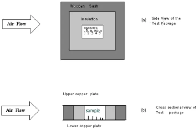
Fig. 2: Test Container, (a) Side View, (b) Cross Section

In order to fix the container inside the test duct to perform cooling process, two pairs of insulated hooks were attached to the inside of the upper and lower surfaces of the test section. The test container was fastened to the upper and lower hooks with the help of thin cotton threads to avoid heat conduction. The characteristic length, x0, of the fish sampled was half

the thickness of the test container (1.27cm). Five copperconstantan thermocouple beads were installed inside the fish flesh, at the depths x0/5, 2x0/5, 3x0/5,

4x0/5 and x0 from the sample surface. In order to make

it possible to insert the temperature sensors at the desired depths, five fine holes were drilled at equal distances of 5 mm from each other in the middle of one copper sheet cover of the test container. The temperatures inside the fish flesh and the dry bulb and wet bulb temperatures of the circulating air were measured with the help of copper constantan thermocouples. The lead wires of all the thermocouples were connected with data logger to obtain the temperature measurements at a specified equal time interval, which was maintained at 1 minute while time of each experiment was 60 minutes. First the refrigeration system of the chilling duct was run until a constant temperature of 1°C was achieved.

Fig. 3: Coordinate System during Precooling

Then the fish package was suspended in the test section of the air duct such that the conducting surfaces were parallel to the direction of flow of the chilled air stream. The data logger was used to collect the transient temperature time data.

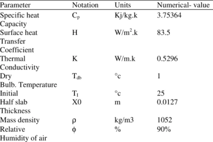
Computational procedure: The system of Equations (1)-(13) was solved for predicting temperature time variations during cooling of solids with pure convection heat transfer from the surface of the solids. The coordinate system for the fish package is shown in Fig. 3 and the mesh of time and space intervals during the finite difference solutions are in Fig. 4. In order to establish a finite difference scheme parameters which are accurate, reliable and efficient for heat transfer analyses during precooling of an infinite slab shaped body, a sample set of temperature-time data was chosen from the experimental work with relevant calculated thermo physical properties of Pangasius Sutchi fish as listed in Table 1. Calculations have been done for air-cooling with only heat transfer boundary condition.

The scheme was found to be stable when

( )

2

X 2

∆ ≥

∆τ

and yield accurate results for all

the space divisions.

Table 3 shows the variation of n with processing time and accuracy at constant stability criterion of (6). The change in n from 5 to 100, only a 0.8 % decrease in error was observed whereas the time elapsed for developing the result will be increased by 72 times.

The experimental results for this slab shaped sample during its air blast cooling considering only heat transfer (such as in canning and tinning) were compared to all the possible explicit finite difference schemes. The concept of least mean root square method of the error has been used which can be represented by the following model:

m

2

E P

i 1

1

S (T T )

m =

Fig. 4: The mesh of time and space intervals during the finite difference solutions

Table 1: Data for Precooling of a Slab Shaped Fish Sample Parameter Notation Units Numerical- value Specific heat Cp Kj/kg.k 3.75364

Capacity

Surface heat H W/m2_{.k 83.5}

Transfer Coefficient

Thermal K W/m.k 0.5296

Conductivity

Dry Tdb °c 1

Bulb. Temperature

Initial TI °c 25

Half slab X0 m 0.0127

Thickness

Mass density ρ kg/m3 1052

Relative φ % 90%

Humidity of air

In the above equation, TE is the experimental value

of temperature. The constant m represents the number of data points and S is the arithmetic mean of root square errors.

RESULTS AND DISCUSSION

First, the fully explicit scheme was examined by substituting θ = 0 in Eq. (5)[10]. A program has been developed in visual Fortran for the system of equations (1-13,16) to predict the temperature distributions verse time in five locations inside the sample to compare the predicted values with the experimental results as shown in Fig. 5. For the investigation of stability criterion

2

( X)∆

∆τ . The program was repeated many times to

determine the optimum value of that criterion on the basis of stability, processing time and accuracy as shown in the Table 2.

The temperature distribution during the cooling test have been compared with that developed by the author’s scheme to show the verification of these schemes among the existing schemes which show good agreement with the experimental results from the time of 9 minutes up to the end (Fig. 6-9).

The proposed scheme was somewhat not accurate for the space Coordinate X≥0. 6 when compared with the other regions as shown in Fig. 10.

Fig. 5: Experimental values of temperature distribution throughout the flash sample

Fig. 6: Deviation of the predicted temperature from the experimental values at X =0

Fig. 7: Deviation of the predicted temperature from the experimental values at X =X0/5

Although Fig. 11 reveals that the sensor location plays the significant role in the obtainable accuracy of the present scheme, the incorporated error could be decreased by discarding the time test up to τ= 0.2 and selecting appropriate (∆X)2

/

∆τ

and n. It is notable to mention that the sensor location in the centerline of the sample yields accurate values whereas the sensor located at 3x0/5 from the sample surface yields an

119 Table 2: The Incorporation of the Relevant Parameter at n=100

2

( X)∆

∆τ 2 4 6 8 10 50 100

Processing 1 1.52 2 2.57 2.97 13.29 26.36 Error 0.22263 0.22267 0.22329 0.22279 0.22283 0.22401 0.22693 *Processing Time Expressed as Index

Table.3: The Incorporation of the Schemes Parameter at (∆X ) 2 _{/∆τ =6}

N 5 10 20 50 100 400

Processing time 1 3 4 19.2 72 23100

Error 0.23522 0.23415 0.22507 0.22335 0.22329 0.22985 *Processing Time Expressed as Index

Fig. 8: Deviation of the Predicted Temperature from the Experimental Values at X =2X0/5

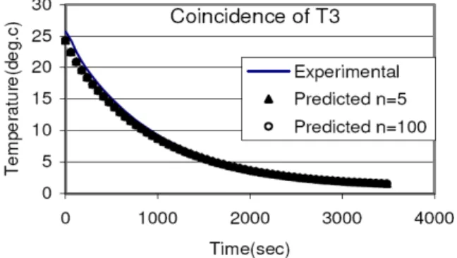
Fig. 9: Deviation of the Predicted Temperature from the Experimental Values at X =3X0/5

Fig. 10: Deviation of the Predicted Temperature from the Experimental Values at X =4X0/5

Fig. 11: The error variation with sensors locations and average throughout the sample

CONCLUSION

On the basis of thorough heat investigations performed in the present study by the explicit finite difference scheme, it can be concluded that:

• The simple explicit finite difference scheme with n = 10 and (

∆

X) 2

/

∆τ

gives reliable and accurate results for making thorough heat analyses during air blast precooling of an infinite slab shaped packages of Freshwater Pangasius Sutchi Fish • As n increases, the accuracy will increase up to

n=100 and beyond this value the accuracy will start decreasing

• The processing time increases, strongly with n • The predicted temperature in this scheme is as

accurate as nearer to the center of the sample • The proposed scheme is recommended for the

space Coordinate 0 ≤ X≤ 0.6 and 9 ≤ t ≤ 60

Nomenclature:

Bi Biot number (h. xo/k) E Error

H surface film conductance (W/m2.K) E Error

K thermal conductivity of product (W/m.K) T temperature (K)

120 U dimensionless temperature [(T- Tcm)/(Ti- Tcm)]

S Error criterion

X dimensionless space coordinates (x/x0) x distance from center (m)

xo

half thickness of infinite slab

τ

Fourier number

(

α

. T/xo

2

)

α

Thermal diffusivity of product

(m

2

/s)

Subscripts:

cm cooling medium db dry bulb I initial E Experimental P Predicted

REFERENCES

1. Ansari, F.A., 1984. Heat and mass transfer analysis in cold preservation of food, pH. D. Thesis, University of Roorkee, India.

2. Ansari, F.A., 1999. Finite difference solution of heat and mass transfer problems related to precooling of food, Energy Conversion and Management, 40: 795 – 802.

3. Baird, C. D. And J. J. Gaffney, 1976. A numerical procedure for calculating heat transfer in bulk loads of fruits and vegetables, ASHRAE Transaction, 82: 525 - 540.

4. Hayakawa, K.I., 1972. Estimating temperatures of foods during various heating or cooling treatments, ASHRAE, J. 14: 65-70.

5. Narayana, K.B. and K. M.V. Murthy, 1977. Heat and Mass Transfer Characteristics and the Evaluation of Thermal Properties of Moist Spherical Bodies, Proceeding of the 4th National Conference on Heat and Mass Transfer, Roorkee, India, 21-23 November.

6. Riclitmyer, R.D. and K.W. Morton, 1967. Difference methods for initial value problems, 2nd edition., New York, Interscience.

7. Berezin, I. S. And M. P. Zhidkov, 1965. Computing Methods. Vol. 1. Reading, Massachusetts, Addison Wesley.

8. Sweat, V.E., 1975. Modelling the thermal conductivity of meats, Transaction of ASAE, 18: 564-568.

9. Riedel L., 1957. Kalorimetri Sche untersuchngen uber das Getriven Von Fleish, Kalte Technik. 9: pp. 38.