Improvement on the sales forecast accuracy for a fast growing company by the best combination of historical data usage and clients segmentation

(1)

ESCOLA BRASILEIRA DE ADMINISTRAÇÃO PÚBLICA E DE EMPRESAS MESTRADO EXECUTIVO EM GESTÃO EMPRESARIAL

IMPROVEMENT ON THE SALES FORECAST ACCURACY FOR A FAST GROWING COMPANY BY THE BEST

COMBINATION OF HISTORICAL DATA USAGE AND CLIENTS SEGMENTATION.

SANTIAGO BURGADA MUÑOZ

Rio de Janeiro - 2014

DISSERTAÇÃO APRESENTADA À ESCOLA BRASILEIRA DE ADMINISTRAÇÃO

(2)

FUNDAÇÃO GETÚLIO VARGAS

ESCOLA BRASILEIRA DE ADMINISTRAÇÃO PÚBLICA E DE EMPRESAS

SANTIAGO BURGADA MUÑOZ

IMPROVEMENT ON THE SALES FORECAST ACCURACY FOR A FAST GROWING COMPANY BY THE BEST COMBINATION OF HISTORICAL DATA USAGE AND CLIENTS SEGMENTATION.

Dissertação de Mestrado apresentada à Escola Brasileira de Administração Pública e de Empresas da Fundação Getúlio Vargas como requisito parcial para a obtenção do título de Mestre em Gestão Empresarial.

Orientador: Prof. Dr. José Mauro Gonçalves

(3)

(4)

Ficha catalográfica elaborada pela Biblioteca Mario Henrique Simonsen/FGV

Burgada Muñoz, Santiago

Improvement on the sales forecast accuracy for a fast growing company by the best combination of historical data usage and clients segmentation / Santiago Burgada Muñoz. – 2014.

94 f.

Dissertação (mestrado) - Escola Brasileira de Administração Pública e de Empresas, Centro de Formação Acadêmica e Pesquisa.

Orientador: José Mauro Gonçalves.

Inclui bibliografia.

1. Previsão de vendas. 2. Segmentação de mercado. 3. Análise de séries

temporais. I. Nunes, José Mauro Gonçalves. II. Escola Brasileira de Administração

Pública e de Empresas. Centro de Formação Acadêmica e Pesquisa. III. Título.

(5)

ABSTRACT

Industrial companies in developing countries are facing rapid growths, and this requires having in place the best organizational processes to cope with the market demand.

Sales forecasting, as a tool aligned with the general strategy of the company, needs to be as much accurate as possible, in order to achieve the sales targets by making available the right information for purchasing, planning and control of production areas, and finally attending in time and form the demand generated.

The present dissertation uses a single case study from the subsidiary of an international explosives company based in Brazil, Maxam, experiencing high growth in sales, and therefore facing the challenge to adequate its structure and processes properly for the rapid growth expected.

Diverse sales forecast techniques have been analyzed to compare the actual monthly sales forecast, based on the sales force representatives’ market knowledge, with forecasts based on the analysis of historical sales data.

The dissertation findings show how the combination of both qualitative and quantitative forecasts, by the creation of a combined forecast that considers both client´s demand knowledge from the sales workforce with time series analysis, leads to the improvement on the accuracy of the company´s sales forecast.

(6)

TABLE OF CONTENTS

ABSTRACT ... I

TABLE OF CONTENTS ... IV

LIST OF FIGURES ... VI

LIST OF TABLES ...VII

1 INTRODUCTION ...9

1.1 Objective ... 9

1.2 Justificative ... 9

1.3 Research hypothesis ... 10

1.4 Research methodology ... 10

1.5 Dissertation structure ... 10

2 FRAME OF REFERENCE ... 12

2.1 Demand forecasting techniques ... 12

2.1.1 Qualitative or judgmental techniques ... 13

2.1.2 Quantitative or statistical techniques ... 14

2.2 Sales demand forecasting ... 15

2.3 Temporal series analysis ... 17

2.3.1 Stationary time series ... 17

2.3.2 Non-stationary time series ... 18

2.3.3 Seasonal time series ... 19

3 COMPANY DEMAND FORECAST... 20

3.1 Clients` segmentation ... 20

3.2 Products segmentation... 21

3.3 Actual monthly sales forecast method. ... 23

4 METHODOLOGY ... 25

4.1 Real sales ... 29

4.2 Proposed forecast models ... 29

4.3 Residues ... 31

4.4 Calculating the best forecast model ... 32

4.5 Comparison of the new residues obtained ... 32

5 RESULTS OBTAINED ... 34

5.1 Minor residue forecast... 34

(7)

6 COMPARISON SALES FORECAST VERSUS PROPOSED FORECAST METHOD ... 41

6.1 First criteria: Minor sum of total residues ... 41

6.2 Second criteria: Compliance with deviations from sales minor than 20 % ... 42

6.3 Third criteria: Total cost reduction ... 44

6.3.1 Potential over-stocks ... 44

6.3.2 Potential sales lost ... 45

6.4 Summary of comparison criteria ... 46

7 CONCLUSIONS ... 48

8 RECOMMENDATIONS ... 49

9 REFERENCES ... 51

(8)

LIST OF FIGURES

Figure 2-1. Main forecast techniques ... 12

Figure 2-2: Sales demand forecasting framework ... 15

Figure 2-3: Stationary time series ... 18

Figure 2-4: Non-stationary time series or trend time series ... 18

Figure 2-5: Seasonal time series ... 19

Figure 3-1: Client´s segmentation ... 21

Figure 3-2: Product´s segmentation... 22

Figure 3-3: Company sales categories analyzed. ... 23

Figure 4-1: Forecast and residues calculation model. Example ... 26

Figure 4-2: Weighted forecast model and models comparison. Example ... 27

Figure 4-3: Sales and forecast models graphical representation. Example ... 28

Figure 4-4:Minor residue model calculation ... 31

Figure 4-5: Weighted forecast model calculation... 32

Figure 4-6: Actual versus new model residues comparison ... 32

Figure 4-7: Graphic comparison actual versus proposed forecast model ... 33

Figure 10-1: Real sales and forecast comparison Booster < 400 g ... 55

Figure 10-2: Real sales and forecast comparison Booster > 400 g ... 58

Figure 10-3: Real sales and forecast comparison Plain detonators ... 61

Figure 10-4: Real sales and forecast comparison Detonating cord < 6 g/m ... 64

Figure 10-5: Real sales and forecast comparison Detonating cord > 6 g/m ... 67

Figure 10-6: Real sales and forecast comparison Non electric det LP ... 70

Figure 10-7: Real sales and forecast comparison Non electric det MS < 9m ... 73

Figure 10-8: Real sales and forecast comparison Non electric det MS 9m a 18 m ... 76

Figure 10-9: Real sales and forecast comparison Non electric det MS > 18 m ... 79

Figure 10-10: Real sales and forecast comparison Non electric det SC ... 82

Figure 10-11: Real sales and forecast comparison Det cord relays... 85

Figure 10-12: Real sales and forecast comparison ANFO ... 88

Figure 10-13: Real sales and forecast comparison Emulsion < 45 mm ... 91

(9)

LIST OF TABLES

Table 5-1: Minor deviation forecast models for all categories... 35

Table 5-2: Minor deviation forecast models for initiation systems ... 36

Table 5-3: Minor deviation forecast models for explosives ... 37

Table 5-4: Weighted forecast model ... 38

Table 5-5: Weighted forecast model. Summary of weights ... 40

Table 6-1: Total residue comparison traditional Vs. weighted forecast model ... 42

Table 6-2: Compliance deviations minor than 20%. Comparison traditional Vs. weighted forecast model ... 43

Table 6-3: Potential over-stocks. Comparison traditional versus weighted forecast model ... 44

Table 6-4: Potential sales lost. Comparison traditional Vs. weighted forecast model ... 45

Table 6-5: Summary of compliance criteria for new forecast method ... 47

Table 10-1: Forecast model analysis for family of products Booster < 400 g ... 53

Table 10-2: Weighted forecast model for family of products Booster < 400 g ... 54

Table 10-3: Forecast model analysis for family of products Booster > 400 g ... 56

Table 10-4: Weighted forecast model for family of products Booster > 400 g ... 57

Table 10-5: Forecast model analysis for family of products Plain detonators ... 59

Table 10-6: Weighted forecast model for family of products Plain detonators... 60

Table 10-7: Forecast model analysis for family of products Detonating cord < 6 g/m... 62

Table 10-8: Weighted forecast model for family of products Detonating cord < 6 g/m ... 63

Table 10-9: Forecast model analysis for family of products Detonating cord > 6 g/m... 65

Table 10-10: Weighted forecast model for family of products Detonating cord > 6 g/m ... 66

Table 10-11: Forecast model analysis for family of products Non electric det LP ... 68

Table 10-12: Weighted forecast model for family of products Non electric det LP ... 69

Table 10-13: Forecast model analysis for family of products Non electric det MS < 9m ... 71

Table 10-14: Weighted forecast model for family of products Non electric det MS < 9m ... 72

Table 10-15: Forecast model analysis for family of products Non electric det MS 9m a 18 m . 74 Table 10-16: Weighted forecast model for family of products Non electric det MS 9m a 18 m 75 Table 10-17: Forecast model analysis for family of products Non electric det MS > 18 m ... 77

Table 10-18: Weighted forecast model for family of products Non electric det MS > 18 m ... 78

Table 10-19: Forecast model analysis for family of products Non electric det SC ... 80

Table 10-20: Weighted forecast model for family of products Non electric det SC ... 81

(10)

Table 10-22: Weighted forecast model for family of products Det cord relays ... 84

Table 10-23: Forecast model analysis for family of products ANFO ... 86

Table 10-24: Weighted forecast model for family of products ANFO... 87

Table 10-25: Forecast model analysis for family of products Emulsion < 45 mm ... 89

Table 10-26: Weighted forecast model for family of products Emulsion < 45 mm ... 90

Table 10-27: Forecast model analysis for family of products Emulsion > 45 mm ... 92

(11)

1 INTRODUCTION

The purpose of this chapter is to introduce the dissertation´s main objective, it´s utility, a first introduction to the research method chosen and the general methodology employed.

1.1 Objective

The dissertation presented has been developed as a simple action oriented case study, being the main objective of this project to find the most accurate sales forecast method for a growing explosives company established in Brazil.

1.2 Justificative

Cerullo and Avila (1975), in a survey of the “Fortune 500 Largest Industrial Companies,” found that 98% of the respondents thought that forecasting should be taught at business schools. Also, sales forecasting was the most common of the nine activities in a survey of 353 marketing directors in British textile firms [Jobber, Hooley and Sanderson (1985)]. As per J. Scott (1989) a content analysis of 53 textbooks on marketing management and marketing research revealed that forecasting was mentioned on less than one percent of the pages. (The sample included all relevant books that could be found at the University of Pennsylvania library).

As we can see from the words of the authors above, forecasting models are considered relevant for most of the industrial sectors; but still not addressed at the same level as other fields of study. The small contribution of this research will be based on understanding how these kinds of forecasting systems fit into the particularities of the explosives and initiation systems sector, for a fast growing company in Brazil.

The research chosen aims to support the work done at the areas of marketing and operations of the chosen company, Maxam, referred in advance as “the company” or ”the firm”.

The company manufactures and supplies industrial explosives and initiation systems to the mining, quarrying and civil works markets in Brazil. It is relatively new into the country, being operating in Brazil since 2007 and experiencing significant yearly growths in sales.

We need to better understand to what extent the client´s demand that is unattended is due to a poor demand forecasting method and/or to a lack of manufacturing capacity, distribution or structure capabilities, or to any other external factors.

(12)

The knowledge acquired through the project will be useful before implementing any specific software available for these purposes; at the same time, as a company case study, may be useful for some other subsidiary operations aiming to have a better understanding of the factors affecting sales demand into the explosives´ sector.

1.3 Research hypothesis

The research purpose is to explore how the usage of historical sales data, at sub-group sales

family level, combined with clients ‘demand knowledge will improve the level of accuracy of the firm´s sales forecast, compared to an actual sales forecast mainly based on sales targets, for a company like Maxam, involved into a fast growing process and getting higher market share.

1.4 Research methodology

For this purpose, the following secondary goals need to be achieved:

1. Improvement on the actual monthly sales forecast data base, facilitating comparative analysis.

2. Establishment of a comparative monthly sales forecast based on historical sales data and client´s demand knowledge. The most suitable model has been created as a combination of time series analysis and sales knowledge derived from clients partitioning and sales workforce knowledge.

3. Analysis of actual and comparative sales forecasts accuracy, understood as deviations from real sales, for the product families already established.

The study will mainly use internal data from the firm´s sales data base, clients´ product demand, and monthly sales forecast prepared by sales and marketing departments.

To measure the accuracy of the sales forecast, our main variable of study, we will compare on a monthly basis the real sales figure - at sub-family of products level - with the sales forecast from commercial department, and with the upgraded proposed forecast that will combine historical sales data with client´s sales demand data.

Data will be mainly treated on Excel spreadsheets, and the usage of dynamic tables will enable the capture of monthly product sales at item and family levels, its comparison with real sales, and its grouping per client segmentations established. For time series analysis IBM SPSS Statistics 20 software will support data gathering and modelling proposal.

1.5 Dissertation structure

(13)

Second chapter - “Frame reference”- introduces a framework for sales forecasting as part of the most general demand forecasting techniques, and it describes briefly the different qualitative and quantitative forecast techniques.

Chapter three – “Company demand forecast”- explains the actual sales demand forecast process, based on the sales workforce representatives´ knowledge on the different categories of products and clients segmentation.

Chapter four- “Methodology”-establishes the process to obtain the weighted forecast, as a mix of the actual sales forecast with six alternative forecasts based on historical sales analysis, as well as the calculation of deviation from real sales for the different forecasts analyzed.

In chapter five –“Resultsobtained”- we can see a summary of the best forecast techniques, in terms of minimum deviation from sales, and the weighted forecast calculated from them for each family of products analyzed.

Chapter six -“Comparison sales forecast versus proposed forecast method”- makes a comparative analysis of the actual sales forecast with the new forecast proposed, and establishes the three main criteria of comparison, that are: minimizing the total residue obtained, adherence to the company maximum deviation target established, as well as final cost reduction.

(14)

2 FRAME OF REFERENCE

In this chapter we will review the main theoretical terms related to the dissertation scope, and their relationship. It starts with a brief review on the most general demand forecasting techniques, to move later on to sales forecast framework, as part of demand forecasting, and finishing with a short introduction to time series data, representing the most common way to observe the data behavior through the time.

2.1 Demand forecasting techniques

The importance of forecasting is highly recognized among marketing practitioners (Cerullo and Avila, 1975), nevertheless as mentioned by J. Scott (1987) the number of research and academic case studies dedicated to this theme is relatively small, compared to other marketing fields of study.

The objective of this chapter is to give a short summary of the dissertation´s field of study, starting with a brief introduction to demand forecasting techniques, and focusing in the next chapter into the more specific sales demand´s forecast methods inside them.

There are two main lines of forecast techniques depending on the usage and availability of quantitative data to be analyzed, and those that rely on judgment or qualitative data, as it can be seen on the diagram below from J. Scott (2012):

Figure 2-1. Main forecast techniques

Source: J.Scott (2012)

(15)

2.1.1 Qualitative or judgmental techniques

These techniques are based on individual or group opinions and qualitative data obtained from them. They are especially useful when there are not enough data, for instance in forecasting the usage of new lines of products non-existent into the market, or when opinions are important in the forecasting decision process. They have a natural bias derived from their own origin and source of information. These techniques have been mainly studied by psychology and related field experts, being the main techniques shown below.

a) Expert surveys

These are usually related to opinion on decision making processes, or to address complex questions.

Experts share their knowledge giving reasoning for their forecasts on the subject.

Opinions or judgment mainly based on sales forces are common, by gathering specialists forecast on the products and markets where those products are applied (Fernando Augusto Silva Marins, 2013), and integrating knowledge from people from different positions, being the Delphi method the most usually known (Makridakis S. and S.C. Wheelwright 1989).

b) Structured analogies

It uses a formal process to compare and use experts’ knowledge on analogous situations to

the one being forecasted or considered as the target forecast.

c) Judgmental decomposition

It implies dividing the forecasting problem into multiplicative parts, for instance the typical sales forecasts based in the multiplication of industry sales times market share forecasts to calculate the company sales forecast. (J. Scott Armstrong, Roderick J. Brodie, Shelby H. McIntyre 1987)

d) Judgmental bootstrapping

It uses experts’ subjective judgments to make a prediction model, usually for complex forecasting models, like new product demands forecast.

e) Expert systems

These systems are created after analyzing and structuring the experts´ rules used for forecasting.

f) Simulated interaction

It´s derived from role-playing techniques, especially useful in decision making processes like those needed on conflict solution processes.

(16)

Related to purchasing or behavioral decisions based on the previous analysis of surveys of the intentions or expectations of the potential consumers. These methods are especially useful when there are no previous data on new products or new market demands. Experimentation methods are usually used to test different product introductions, through field or laboratory programs.

2.1.2 Quantitative or statistical techniques

These techniques use quantitative data and statistical tools for its compilation and analysis. They have been deeply studied by economists, being econometrics the main field of study.

a) Extrapolation models

These models use historical data of the variable to be forecasted, not considering causal factors. Econometric models are fitted into this category.

They involve the numerical analysis of historical data, being their main subdivision the time series analysis, consisting on the prediction of future sales as per the best model fitting with historical sales for a considered time frame. Time series can be categorized as stationary, trend based and seasonal, being the main known forecast methods the moving average, regression and exponential smoothing.

These methods will be explained in detail as an independent chapter of this document, as they form the basis of the actual project study being combined with qualitative techniques , mainly expert surveys, in place.

b) Quantitative analogies

This method is used when there are no enough data of the demand variable, and in this case data from analogous demand situations may be used to extrapolate the forecast.

c) Rule-based forecasting

This model integrates managers’ knowledge with time series forecasts. Somehow this model is followed by the company into their forecast process;, but not being structured in a formal process.

d) Neural nets

These methods try to find out nonlinear patterns in time series analysis.

e) Causal methods

(17)

Regression analysis, to find the dependence between the variable of study and one or more causal variables, are frequently used, and index method in which there is a little knowledge on the variable of study but greater knowledge on the causal variables

f) Segmentation

Uses the combination of different segments driven by different causal variables and adding the independent forecasts for each segment.

Finally, not included in the tree diagram of figure 2-1, we can find the simulation methods, consisting in the development of a dynamic method in which all the internal and external variables affecting the demand are established and alternative scenarios simulated to predict future demands.

2.2 Sales demand forecasting

We can see below how sales demand forecasting fits into the general business strategy of the company as adapted from Makidrakis (1989)

Figure 2-2: Sales demand forecasting framework

(18)

The business strategy of the company starts with the long term planning or strategic planning, covering periods of approximately three to five years and cascading down to medium term planning ,or aggregate planning, usually covering the actual year´s forecast. Inside the latter, item forecasting focuses in the short term (weeks or months). This part of the business strategy planning is the framework of the present dissertation.

Sales forecast is therefore a critical part of the global company strategy, translating the original broader perspective into detailed production schedules, sales targets and finally, adherence to yearly budgets and results.

Due to the nature of the industrial sector on study, it is highly regulated and most frequently controlled by the government administration per security reasons, therefore information on explosives´market sales data is not found available easily. Market size is obtained indirectly, mainly through end users usage, like mining, quarrying or construction works usage of explosives, installed market capacities of raw materials needed to be converted into explosives (mainly ammonium nitrate) , or some other indirect methods.

Typical sales forecasts based in the multiplication of industry sales and market share forecasts to calculate the company sales forecast (J. Scott 1987), will be therefore more difficult to be done, and direct sales forecast are more common. It must be pointed out that this approach is not unique from this sector, in line with studies like the one developed by

Dalrymple’s (1987) and others, especially when treating with short- range sales forecasting. For the above fore mentioned reasons, sales forecast models are usually based on a mix of quantitative and qualitative methods, being the most common the analysis of historical sales series (historical data as time series) as well as sales representatives market knowledge and previsions, as confirmed by Wotruba and Thurlow (1976), rather than models purely based on market demand.

It needs to be considered the possibility of isolating the bias from the sales force executives from other errors (Staelin and Turner, 1972), as this can be responsible for up to 60% of the forecast error as expressed by J. Scott (1987)

We can find different opinions in the forecast literature in favor of quantitative extrapolation methods or qualitative judgmental ones, “Lawrence et al. (1985) concluded in favor of judgmental or “eyeball” extrapolations, but Carbone and Gorr (1985) and Mabert (1976) concluded the opposite” as concluded by J Scott (1987)

Nevertheless we can also find a bigger number of studies supporting the mix of both methods to obtain a more accurate sales forecast, Baker et al. (1980), Sewall (1981) or even Lawrence et al. later (1986), as compiled by J. Scott (1987)

(19)

Behavioral economists have also demonstrated that, judgmental forecasts have intrinsic value and, combined with quantitative forecasts, improve overall forecast accuracy as per Thomas Oriol (2013) studies.

There are also interesting study lines like that from Schnaars (1986) that establishes various rules to select the most appropriate extrapolation method, against the general rule of selecting the one that best fits with the historical sales data.

In the present dissertation, it will be studied the best combination of both quantitative and qualitative methods to deliver a combined method that best fits with the historical sales data and minimizes the error, understood as the absolute value of the difference between real sales and forecast.

2.3 Temporal series analysis

A temporal series is the result of observing a variable´s value through the time at regular time intervals (daily, monthly, yearly, etc.) (Daniel Peña 2010)

Time series analysis will support the prediction of future sales, as it looks for the best model fitting with historical sales, for a considered time frame.

Those series oscillating around an even level are considered stationary, and those that aren´t will be classified as non-stationary, or trend based.

Any of the above series that also have a behavior that replies through the time are considered seasonal.

2.3.1 Stationary time series

(20)

Figure 2-3: Stationary time series

Source: Makidrakis (1989)

2.3.2 Non-stationary time series

The values of the series don´t oscillate around an even value, but it can exist a tendency to grow or decrease with the time.

An example of these kind of series can be found in the graphic below:

Figure 2-4: Non-stationary time series or trend time series

(21)

2.3.3 Seasonal time series

The values of the series follow a time cycle, for instance the monthly temperatures through the year.

An example of these kind of series can be found in the graphic below

Figure 2-5: Seasonal time series

Source: Makidrakis (1989)

In the present dissertation we will focus on the analysis and construction of a model that best represents the evolution of the temporal sales series and will predict its future behavior, or future values, this is, the best fitting sales forecast.

These models are classified as uni-variant as they are based uniquely on the temporal history of the series. The predictions obtained through these models are based on the hypothesis that future conditions will be similar to those happened in the past, and they are especially useful when forecasting in the short term, like the case in study, in which we will forecast monthly sales.

The models used will differ on the shape of the line that best fits with the observed data, being moving average, regression and exponential smoothing the most commonly used.

(22)

3 COMPANY DEMAND FORECAST

Company sales and demand forecast are mainly segmented by three criteria, being these product segmentation, type of clients - either existing or potential ones - as well as per geographical location.

3.1 Clients` segmentation

The clients’ segmentation is at the same time also based on three criteria: 1) Group.

Defines the size of the client´s revenue, but also potential revenues or strategic importance for the company.

There are 6 main groups established:

Group 1: Big clients (GC)

Group 2: Medium clients (MC)

Group 3: Distributors (Distr)

Group 4: Exports (Exp)

Group 5: Direct sales (VD)

Group 6: Other sales (O)

2) Division.

Defines the name of the client in the case of big and medium clients, and regional area for the rest of the groups.

3) Market.

Defines the type of market in which the client operates, being the main ones the following:

Market 0: Specialized markets (“Mercados especializados”)

Market 1: Quarries (“Pedreiras e Calcáreos”)

Market 2: Mining (“Mineradoras”) Market 3: Coal (“Carvão”)

Market 4: Projects (“Projetos”)

(23)

Market 9: Competitors (“Concorrentes”)

We can see an example of this division below, and a summary table of client´s classification

Client Kinross (1.4.2):

Group 1: Big client

Division 4: Name of the client

Market 2: Mining (Mineradoras)

Figure 3-1: Client´s segmentation

Source: Own elaboration

During the period analyzed at the dissertation (November 2011 to June 2014) the total number of active clients was two hundred and sixty one (261), being twelve (12) of them classified as big or medium clients, amounting for 71% of the total sales in value.

3.2 Products segmentation

Products are divided in two main groups, initiation systems and explosives, sub-grouped in six (6) and three (3) sales groups. Each sales group is subdivided into sales categories commonly named product families, totaling 20 sales categories as shown in the figure below:

Agrupamentos & Divisões

GC 1 0 Vale Dist 3 0 reg 0 - SP, RJ, ES VD 5 0 reg 0 - SP, RJ, ES 0 Mercados Especializados 1 Holcim 1 reg 1 - MG, BA 1 reg 1 - MG, BA 1 Pedreiras & Calcáreos

2 CSN 2 reg 2 - PR, SC, RS 2 reg 2 - PR, SC, RS 2 Mineradoras

3 Votorantim 3 reg 3 - MS, MT, GO 3 reg 3 - MS, MT, GO 3 Carvão

4 Kinross 4 reg 4 - Nordeste 4 reg 4 - Nordeste 4 Projetos

5 5 reg 5 - Norte, incl TO 5 reg 5 - Norte, incl TO 5 Revenda/Distribuidores

6 6 6 6

7 7 7 7

8 8 8 8

9 Outros 9 Concorrentes 9 Concorrentes 9 Concorrentes

MC 2 0 Yamana Exp 4 0Latam - Bolivia O 6 Outros

1 Brasitalia/Concresul 1 Latam - Peru/Chile 2 Valle Sul 2 Latam - Equador 3 Jaguar 3 Latam - resto Mercosur 4 Usiminas 4 Latam - resto Andino

5 Lafarge 5 Latam - centro Am

6 Etermar 6 Africa

7 Van oord 7 Estados Unidos

8 8

(24)

Figure 3-2: Product´s segmentation

For academic purposes the analysis of company sales and forecast has been limited to sales category level. Sales categories marked as (1) to (4) inside initiating systems have not been included, as volumes are not significant, as well as sales categories (5) and (6) into the explosives group, as these are forecasted locally at mine sites.

Therefore we will be analyzing the most representative families of products, a total of fourteen (14) sales categories as shown in figure 3.3.

Sales categories are subdivided at item level, or sku (stock keeping unit or “sku”) being 467 skus active during the analysis period of the dissertation.

The family level of aggregation has been considered in order to be able to manage a representative number of data. At aggregate level (sales group) when demand is considered as a whole heterogeneity and variability would be difficult to analyze; at the same time, working at sku level would imply a high number of data and information required.

SALES GROUP SALES CATEGORY DESCRIPTION UOM

BOOSTERS < 400 GRS U

BOOSTERS >= 400 GRS U

CAP FUSE PLAIN DETONATOR U

DETONATING CORD <= 6 gr M

DETONATING CORD 10 / 12 gr M

DETONATING CORD 40 / 60 gr (1) M

DETONATING CORD 80 / 100 gr (2) M

NON ELECTRIC DETONATORS LONG PERIOD U

NON ELECTRIC DETONATORS SHORT PERIOD <= 9 m U

NON ELECTRIC DETONATORS SHORT PERIOD 9 TO <=18 m U

NON ELECTRIC DETONATORS SHORT PERIOD > 18 m U

NON ELECTRIC DETONATORS DUAL DELAY (3) U

NON ELECTRIC DETONATORS SURFACE CONNECTOR U

DETONATING CORD RELAYS U

SAFETY FUSE (4) M

BAGGED ANFO KG

OPEN PIT RIOFLEX (5) KG

OPEN PIT RIOMEX (6) KG

SMALL CARTRIDGES EMULSION < 45 mm KG

MEDIUM CARTRIDGES EMULSION > 45 mm KG

BULK

SALES FORECAST INITIATION SYSTEMS

SALES FORECAST EXPLOSIVES

DETONATING CORD

(25)

Figure 3-3: Company sales categories analyzed.

3.3 Actual monthly sales forecast method.

The sales forecast is prepared in the company on monthly basis by the sales force representatives and project managers, being up to a total of thirteen people involved in the process. Each one of them is responsible for delivering the sales forecast of his/her specific project or regional area.

The sales forecast template is grouped in families of products, and for each area the most representative clients´ sales are estimated at item level (“sku” or stock keeping unit). Those clients not being so representative in terms of sales, are grouped as an additional group (others).

This area/project sales forecast is mainly based on the client´s sales demand communicated, as well as on the sales force market knowledge.

The marketing department will add all the partial forecasts and will compare, usually at family group level, with the historical sales data, as well as with the sales targets established. After this, a revision of the forecast is done with each sales or project representative to agree on the final monthly sales forecast.

The monthly sales forecast is somehow considered as a sales target to be achieved by each sales representative or project responsible. This fact can add some bias to the expected sales forecast, as original data can be increased due to the expectance on achieving the sales

BOOSTERS < 400 GRS U

BOOSTERS >= 400 GRS U

CAP FUSE PLAIN DETONATOR U

DETONATING CORD <= 6 gr M

DETONATING CORD 10 / 12 gr M

NON ELECTRIC DETONATORS LONG PERIOD U

NON ELECTRIC DETONATORS SHORT PERIOD <= 9 m U

NON ELECTRIC DETONATORS SHORT PERIOD 9 TO <=18 m U

NON ELECTRIC DETONATORS SHORT PERIOD > 18 m U

NON ELECTRIC DETONATORS SURFACE CONNECTOR U

DETONATING CORD RELAYS U

BULK BAGGED ANFO KG

SMALL CARTRIDGES EMULSION < 45 mm KG

MEDIUM CARTRIDGES EMULSION > 45 mm KG

SALES FORECAST INITIATION SYSTEMS

SALES FORECAST EXPLOSIVES

BOOSTERS

DETONATING CORD

(26)

targets established; at the same time some sales force could be tempted to decrease the sales expected, not creating this way big sales expectations to be committed to achieve later on.

This phenomenon has been deeply studied , and can be responsible for up to 60% of the forecast error, as expressed by J. Scott (1987)

These facts make the forecast useful as a sales tool inside the sales department, but it must be observed and used carefully by the rest of the company areas, like the operations department in charge of the planning, control and production, especially at the time of calculating the real purchases and stock levels needed to attend the forecasted demand.

It´s quite common that the operations department will base its purchases of raw materials and manufacturing plan as per historical sales data rather than per sales forecast, especially when the latter shows big differences with the real sales during the previous months of study.

It´s therefore crucial to make the sales forecast more accurate, so that it could be widely used throughout all the company departments. This is the core of the present dissertation, in which we will try to find the right combination of qualitative input from the sales force mixed with a pure quantitative forecast based on the analysis of the sales time series.

The universe of study is all the explosives and initiation systems forecasted on monthly basis and the real sales figure (in quantities) for the same period. In number of items, this would represent around 300 items/month. The sample of study will be the sub-group of family item level, composed of 14 families, as shown previously in figure 3.3.

(27)

4 METHODOLOGY

As described in previous chapters the main objective of the dissertation analysis is to find out the best sales forecast method, created as a combination of methods, allowing the company to minimize the deviations between sales forecast and real sales figures.

The process consists in the comparative analysis of the historical sales data (temporal series analysis) with the sales force forecast, and with six alternative forecast methods, obtaining the deviation of each one against real sales.

The method chosen uses a weighted combination of the actual and alternative forecasts, accordingly to the method that delivers the minimum deviation from sales figure for the period observed.

This comparison has been done at product family level, for each of the fourteen categories established in Figure 3.3.

The period of analysis considered comprises thirty one (31) months starting November 2011 up to June 2014.

Method statement, analysis and calculations are explained below for one of the product categories as an example, (emulsions minor than 45 mm), having included the analysis for the rest of categories at the end of the document, as Annexes, for easier reading and follow up of the document.

We can see in figure 4.1 the template used to compile the results obtained by the calculation of the alternative forecasts, as well as their deviation from the real sales figure for the period observed.

In figures 4.2 and 4-3. we can see the calculation of the weighted forecast model, comparison with the actual forecast model residues, as well as graphical representation of the data obtained.

(28)

Figure 4-1: Forecast and residues calculation model. Example

(29)

Figure 4-2: Weighted forecast model and models comparison. Example

(30)

Figure 4-3: Sales and forecast models graphical representation. Example

(31)

Let’s see each of the terms on the comparative analysis shown in the previous figures in detail:

4.1 Real sales

4.2 Proposed forecast models

These are the six different forecast models to the actual forecast that have been calculated by using the historical sales figures, being the following:

Month Emulsion < 45 mm

nov-11 17900

… …

jun-14 36337

REAL SALES

Aut. Modelling

Arima (LA) c/ c.

Arima (LA)

s/ c. N-1 Sales

Season Trend

Prev. Quarter Sales avg.

MXM Forecast

FORECAST MODEL

Aut.

Modelling

Arima (LA)

c/ c.

Real sales data have been compiled for each of the product categories established, in product units for the observed period, starting November 2011 up to June 2014, In the example: monthly sales data for the family Emulsion < 45 mm

Automatic modelling analyses the historical sales data and calculates the best forecast model fitting with the time series analyzed. Its results have been obtained by the usage of IBM SPSS Statistics 20 Software.

(32)

Arima (LA)

s/ c.

N-1 Sales

Season

Trend

Prev.

Quarter

Sales avg.

MXM

Forecast

Arima (0,1,1) without constant, that calculates the simple exponential smoothing of the data: rather than taking the most recent observation as the forecast of the next observation, it uses an average of the last few observations in order to filter out the noise and more accurately estimate the local mean. The simple exponential smoothing model uses an exponentially weighted moving average of past values to achieve this effect. Its results have been obtained by the usage of IBM SPSS Statistics 20 Software

This simple model consists on considering the previous month sales as the forecast for the next month. It has been calculated through Excel spreadsheet

This model considers the sales growth for the same month of previous year, and applies it to the previous month to get next month forecast; i.e.: Jun 2014 forecast sales = May 2014 sales x (June 2013 sales /May 2013 sales) It has been calculated through Excel spreadsheet

This model considers as forecast for next month the previous quarter average sales. It has been calculated through Excel spreadsheet

(33)

4.3 Residues

In this part of the analysis is calculated the difference, in absolute value, between the real sales figure and the forecast models calculated quantities, this difference is called the residue of the model.

Among all the residues, in the column minor residue model, is selected the value of the model that delivers the minimum residue for each month.

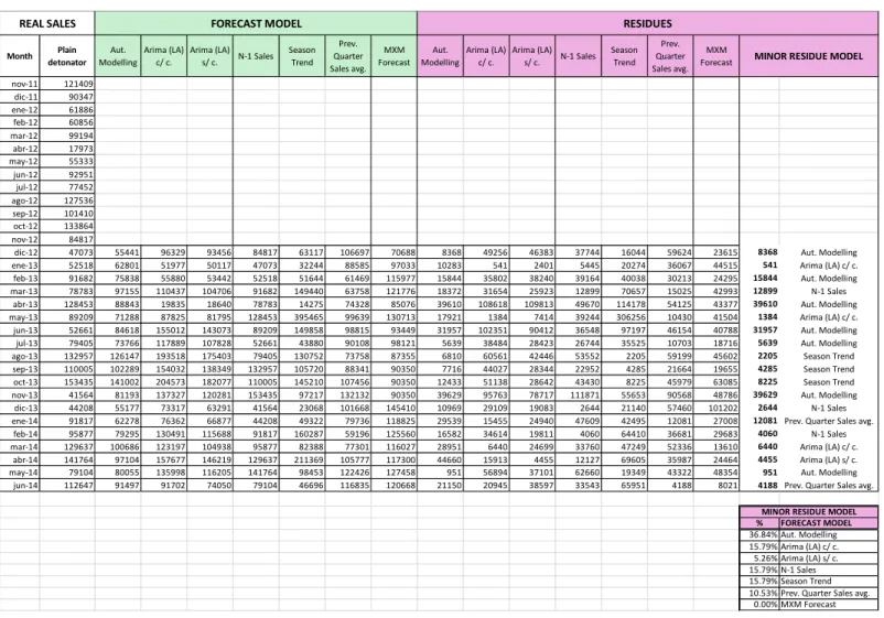
After this process, it is calculated the percentage of occasions for each forecast model in which they have delivered the minor residue model, as in the example shown below:

Figure 4-4:Minor residue model calculation

Aut. Modelling

Arima (LA) c/ c.

Arima (LA)

s/ c. N-1 Sales

Season Trend Prev. Quarter Sales avg. MXM Forecast RESIDUES

MINOR RESIDUE MODEL

8584 93019 89385 2325 69963 1633 15378 1633 Prev. Quarter Sales avg. 485 3388 4687 5425 20346 2608 21794 485 Aut. Modelling 3609 3500 5737 21325 4217 24167 14385 3500 Arima (LA) c/ c. 18389 9104 7626 33100 8204 17075 25892 7626 Arima (LA) s/ c.

251 15065 16305 15165 20878 207 20052 207 Prev. Quarter Sales avg. 12407 4575 5971 4005 4115 4928 6364 4005 N-1 Sales

3552 8147 7006 18885 8801 16500 25898 3552 Aut. Modelling 7903 5243 3530 10250 3658 3675 17797 3530 Arima (LA) s/ c. 1536 23709 21022 1750 15651 1212 4581 1212 Prev. Quarter Sales avg. 1295 12357 9730 4375 4141 6625 45 45 MXM Forecast 3015 21767 18367 2350 8148 4683 2172 2172 MXM Forecast 787 20216 18038 9275 5982 6250 7103 787 Aut. Modelling 12966 13705 10122 1950 350 7350 28700 350 Season Trend 17199 9907 12143 25300 21628 20908 18467 9907 Arima (LA) c/ c.

9051 2461 1005 17925 9110 34142 8400 1005 Arima (LA) s/ c. 29583 46320 48228 12150 48907 32533 7675 7675 MXM Forecast 17494 14503 15786 8925 37792 23000 14100 8925 N-1 Sales 20377 32754 30433 45660 37107 35660 11585 11585 MXM Forecast

4461 6399 8286 3403 17453 30868 62238 3403 N-1 Sales

amily of products Emulsion < 45 mm

% FORECAST MODEL

15.79% Aut. Modelling 10.53% Arima (LA) c/ c. 15.79% Arima (LA) s/ c. 15.79% N-1 Sales

5.26% Season Trend

15.79% Prev. Quarter Sales avg. 21.05% MXM Forecast

(34)

4.4 Calculating the best forecast model

Once calculated the six alternative forecasts to the actual sales forecast, and their respective residues, it is finally calculated the weighted forecast method, that weights all the methods calculated quantities accordingly to the percentage of times that the method was the minor residue model.

In the example above shown, the combined forecast method would be the following:

Figure 4-5: Weighted forecast model calculation

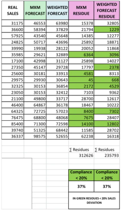
4.5 Comparison of the new residues obtained

Once the new forecast model has been calculated is needed to compare the new residues obtained with the traditional company forecast residues, as it can be seen below:

Figure 4-6: Actual versus new model residues comparison

WEIGHTED FORECAST MODEL = 15.79 % Aut. Modelling + 10.53 % Arima (LA) c/ c. + 15.79 % Arima

(LA) s/ c. + 15.79 % N-1 Sales + 5.26 % Season Trend + 15.79% Prev. Quarter Sales avg. + 21.05 % MXM

Forecast

31175 46553 63980 15378 32805 36600 58394 37829 21794 1229 57925 43540 45648 14385 12277 24825 50717 43696 25892 18871 39990 19938 28122 20052 11868 35985 29621 32889 6364 3096 17100 42998 31127 25898 14027 27350 45147 29728 17797 2378 25600 30181 33913 4581 8313 29975 29930 30643 45 668 32325 30153 36854 2172 4529 23050 30153 32412 7103 9362 21100 49800 33717 28700 12617 46400 64867 36178 18467 10222 64325 72725 57023 8400 7302 76475 68800 48068 7675 28407 85400 71300 72598 14100 12802 39740 51325 68442 11585 28702 36337 98575 52655 62238 16318

∑ Residues ∑ Residues 312626 235793 Compliance < 20% Compliance < 20% REAL SALES MXM FORECAST WEIGHTED FORECAST 37% 37%

IN GREEN RESIDUES < 20% SALES DEVIATION MXM RESIDUE

WEIGHTED FORECAST

RESIDUE The residues for the new proposed model

(weighted forecast residue column) are calculated and compared with the residues for the actual sales forecast method (MXM Residue)

Two aspects are considered into this comparative analysis:

a) The total sum of residues for both methods.

(35)

Finally, for each product family is shown a graphical representation of the data obtained, to compare the actual forecast with the new proposed method, that is the weighted forecast model, showing their deviation with the real sales figure for the period of study.

Figure 4-7: Graphic comparison actual versus proposed forecast model

(36)

5 RESULTS OBTAINED

In this chapter is presented a summary of the forecasts showing the minor residue for the different families of products studied, as well as the weighted forecast calculated

5.1 Minor residue forecast

A total of thirty two months of historical series have been analyzed in order to find out the best sales forecast method for the firm..

The initial period ranging from November 2011 to November 2012 is considered the base for next months calculations.

For each of the fourteen sales categories selected, sales forecast under the new forecast methods analyzed have been created, for the period ranging from December 2012 to June 2014 (Total of nineteen months)

Therefore, for each new forecast method we have got two hundred and sixty six (266) sales forecast monthly data (fourteen (14) sales categories times nineteen (19) months)

We can see in the tables below the methods that have delivered the best data on monthly basis, considered as minimum deviation from sales, for each sales category considered.

Three tables are presented, (tables 5.1-1 to 5.1-3), with the results grouped for all the categories, as well as detailed for explosives and initiation systems.

As it can be observed, the actual sales forecast as well as the automatic modelling are the forecasts that have obtained minor deviation from sales in a major number of occasions.

Forecast based on previous sales that use data in the short term, like previous month sales forecast and previous quarter average sales forecast follow them, and finally Arima methods, as well as season trend method, have given the biggest deviation from sales.

(37)

Table 5-1: Minor deviation forecast models for all categories

Obs: Data in cells representing number of months in which the forecast method chosen delivered the minimum deviation from sales

Source: Own elaboration

FORECAST MODEL Booster < 400 g

Booster > 400 g

Plain detonator

Det Cord < 6 g/m

Det cord > 6 g/m

Non electric

det LP

Non electric det MS <

9m

Non electric

det MS 9m a 18

m

Non electric det MS > 18 m

Non electric

det SC

Det cord relays ANFO

Emulsion < 45 mm

Emulsion > 45 mm Total

% BEST METHOD

Aut. Modelling 5 2 7 2 3 8 6 4 2 2 5 8 3 4 61 22.93%

MXM Forecast 3 6 0 8 7 1 4 5 5 8 3 3 4 4 61 22.93%

Prev. Quarter Sales avg. 2 0 2 2 1 3 2 5 5 3 5 2 3 2 37 13.91%

N-1 Sales 2 5 3 2 3 2 2 1 1 3 4 4 3 2 37 13.91%

Arima (LA) s/ c. 5 2 1 3 2 0 1 2 2 2 1 1 3 2 27 10.15%

Season Trend 2 3 3 0 1 5 2 1 1 0 0 1 1 3 23 8.65%

Arima (LA) c/ c. 0 1 3 2 2 0 2 1 3 1 1 0 2 2 20 7.52%

Total months forecasted 19 19 19 19 19 19 19 19 19 19 19 19 19 19 266 SALES CATEGORY

(38)

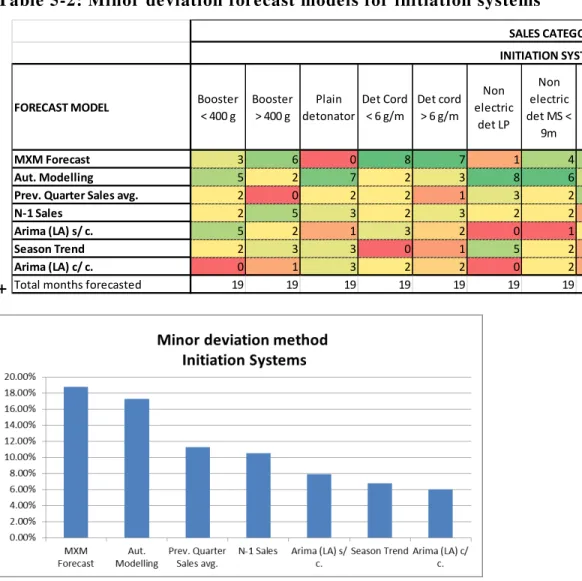
Table 5-2: Minor deviation forecast models for initiation systems

+

Source: Own elaboration

FORECAST MODEL Booster < 400 g

Booster > 400 g

Plain detonator

Det Cord < 6 g/m

Det cord > 6 g/m

Non electric

det LP

Non electric det MS <

9m

Non electric

det MS 9m a 18

m

Non electric det MS >

18 m

Non electric

det SC

Det cord relays Total

% BEST METHOD

MXM Forecast 3 6 0 8 7 1 4 5 5 8 3 50 18.80%

Aut. Modelling 5 2 7 2 3 8 6 4 2 2 5 46 17.29%

Prev. Quarter Sales avg. 2 0 2 2 1 3 2 5 5 3 5 30 11.28%

N-1 Sales 2 5 3 2 3 2 2 1 1 3 4 28 10.53%

Arima (LA) s/ c. 5 2 1 3 2 0 1 2 2 2 1 21 7.89%

Season Trend 2 3 3 0 1 5 2 1 1 0 0 18 6.77%

Arima (LA) c/ c. 0 1 3 2 2 0 2 1 3 1 1 16 6.02%

Total months forecasted 19 19 19 19 19 19 19 19 19 19 19 209 SALES CATEGORY

(39)

Table 5-3: Minor deviation forecast models for explosives

Source: Own elaboration

FORECAST MODEL ANFO Emulsion < 45 mm

Emulsion > 45 mm Total

% BEST METHOD

Aut. Modelling 8 3 4 15 26.32%

MXM Forecast 3 4 4 11 19.30%

N-1 Sales 4 3 2 9 15.79%

Prev. Quarter Sales avg. 2 3 2 7 12.28%

Arima (LA) s/ c. 1 3 2 6 10.53%

Season Trend 1 1 3 5 8.77%

Arima (LA) c/ c. 0 2 2 4 7.02%

Total months forecasted 19 19 19 57 SALES CATEGORY

(40)

5.2 Weighted forecast model obtained

As previously explained, the weighted forecast for each sales category has been established by the ideal combination of the actual forecast with the six alternative forecasts analyzed.

By using the percentages of the best forecast model, delivering minor residues inside the category, the new combined forecast is obtained.

We can see below the weighted forecast obtained for each of the sales categories:

Table 5-4: Weighted forecast model

SALES CATEGORY WEIGHTED FORECAST MODEL

Booster < 400 g 26.32 % Aut. Modelling + 0.00 % Arima (LA) c/ c. + 26.32 % Arima

(LA) s/ c. + 10.53 % N-1 Sales + 10.53 % Season Trend + 10.53 % Prev. Quarter Sales avg. + 15.79 % MXM Forecast

Booster > 400 g 10.53 % Aut. Modelling + 5.26 % Arima (LA) c/ c. + 10.53 % Arima

Plain detonator 36.84 % Aut. Modelling + 15.79 % Arima (LA) c/ c. + 5.26 % Arima

Det cord < 6 g/m 10.53 % Aut. Modelling + 10.53 % Arima (LA) c/ c. + 15.79 %

Arima (LA) s/ c. + 5.26 % N-1 Sales + 0.00 % Season Trend + 10.53% Prev. Quarter Sales avg. + 47.37 % MXM Forecast

Det cord > 6 g/m 15.79 % Aut. Modelling + 10.53 % Arima (LA) c/ c. + 10.53 %

Arima (LA) s/ c. + 15.79 % N-1 Sales + 5.26 % Season Trend + 5.26 % Prev. Quarter Sales avg. + 36.84 % MXM Forecast

Non electric det LP 42.11 % Aut. Modelling + 0.00 % Arima (LA) c/ c. + 0.00 % Arima

Non electric det MS < 9 m 31.58 % Aut. Modelling + 10.53 % Arima (LA) c/ c. + 5.26 % Arima

(41)

Non electric det MS 9 m a 18 m

21.05 % Aut. Modelling + 5.26 % Arima (LA) c/ c. + 10.53 % Arima (LA) s/ c. + 5.26 % N-1 Sales + 5.26 % Season Trend + 26.32 % Prev. Quarter Sales avg. + 26.32 % MXM Forecast

10.53 % Aut. Modelling + 15.79 % Arima (LA) c/ c. + 10.53 % Arima (LA) s/ c. + 5.26 % N-1 Sales + 5.26 % Season Trend + 26.32 % Prev. Quarter Sales avg. + 26.32 % MXM Forecast Non electric det SC 10.53 % Aut. Modelling + 5.26 % Arima (LA) c/ c. + 10.53 %

Det cord relays 26.32 % Aut. Modelling + 5.26 % Arima (LA) c/ c. + 5.26 %

ANFO 42.11 % Aut. Modelling + 0.00 % Arima (LA) c/ c. + 5.26 %

Arima (LA) s/ c. + 21.05 % N-1 Sales + 5.26 % Season Trend + 10.53% Prev. Quarter Sales avg. + 15.79 % MXM Forecast Emulsion < 45 mm 15.79 % Aut. Modelling + 10.53 % Arima (LA) c/ c. + 15.79

% Arima (LA) s/ c. + 15.79 % N-1 Sales + 5.26 % Season Trend + 15.79% Prev. Quarter Sales avg. + 21.05 % MXM Forecast

Emulsion > 45 mm 21.05 % Aut. Modelling + 10.53 % Arima (LA) c/ c. + 10.53 % Arima (LA) s/ c. + 10.53 % N-1 Sales + 15.79 % Season Trend + 10.53% Prev. Quarter Sales avg. + 21.05 % MXM Forecast

(42)

Table 5-5: Weighted forecast model. Summary of weights SALES

CATEGORY

Aut Model

Arima (LA) c/ c

Arima (LA) s/ c.

N-1 Sales

Season Trend

Prev. Quarter Sales avg.

MXM Forecast

Booster < 400 g 26.32 % 0.00 % 26.32 % 10.53 % 10.53 % 10.53 % 15.79%

Booster > 400 g 10.53% 5.26% 10.53% 26.32% 15.79% 0.00% 31.58%

Plain detonator 36.84% 15.79% 5.26% 15.79% 15.79% 10.53% 0.00%

Det cord < 6 g/m 10.53% 10.53% 15.79% 5.26% 0.00% 10.53% 47.37%

Det cord > 6 g/m 15.79% 10.53% 10.53% 15,79% 5.26% 5.26% 36.84%

Non electric det LP

42.11% 0.00% 0.00% 10.53% 26.32% 15.79% 5.26%

Non electric det MS < 9 m

31.58% 10,53% 5.26% 10,53% 10,53% 10,53% 21.05%

Non electric det MS 9 m a 18 m

21.05% 5.26% 10.53% 5.26% 5.26% 26.32% 26.32%

10.53% 15.79% 10.53% 5.26% 5.26% 26.32% 26.32%

Non electric det SC

10.53% 5.26% 10.53% 15.79% 0.00% 15.79% 42.11%

Det cord relays 26.32% 5.26% 5.26% 21.05% 0.00% 26.32% 15.79%

ANFO 42.11% 0.00% 5.26% 21.05% 5.26% 10.53% 15.79%

Emulsion < 45 mm

15.79% 10.53% 15.79% 15.79% 5.26% 15.79% 21.05%

Emulsion > 45 mm

21.05% 10.53% 10.53% 10.53% 15.79% 10.53% 21.05%

(43)

6 COMPARISON SALES FORECAST VERSUS PROPOSED FORECAST METHOD

By using the percentages of the best forecast model inside the category, the new combined forecast have proved better results against the traditional sales forecast in most of the occasions.

Three main parameters have been established to compare the new proposed forecast with the traditional one used in the firm till date.

 Minor sum of total residues

 Compliance with deviations minor than 20% from sales  Total cost reduction

Let´s see details on the data obtained for each of the above parameters:

6.1 First criteria: Minor sum of total residues

This parameter indicates how far the models studied are deviated from the real sales for the period, in absolute values.

It has been calculated by adding the deviations from sales quantities for the period observed (Dec 2012 to June 2014)

It´s important to point out that is common working with forecasts that either minimize the quadratic error of the deviation or the absolute value of the deviations like the case on study, as a way to offset the effect of positive and negative deviations being added and

resulting in a “zero mean deviation”.

The same error positive and negative has different meanings, and adding same value deviations positive and negative could make us extract wrong conclusions (zero mean deviation). Nevertheless, for detailed analysis, we will still use positive and negative deviations, assuming that the first ones could lead to potential overstock for positive deviations (forecast > sales) and potential sales lost if negative (forecast < sales)

(44)

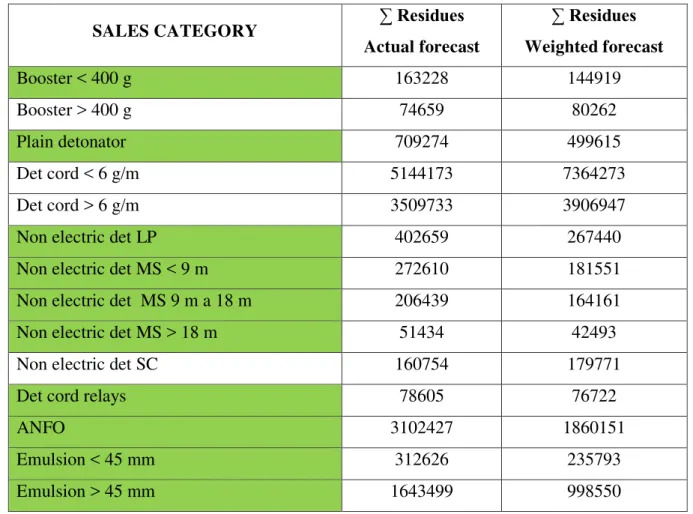
Table 6-1: Total residue comparison traditional Vs. weighted forecast model

SALES CATEGORY ∑ Residues

Actual forecast

∑ Residues

Weighted forecast

Booster < 400 g 163228 144919

Booster > 400 g 74659 80262

Plain detonator 709274 499615

Det cord < 6 g/m 5144173 7364273

Det cord > 6 g/m 3509733 3906947

Non electric det LP 402659 267440

Non electric det MS < 9 m 272610 181551

Non electric det MS 9 m a 18 m 206439 164161

Non electric det MS > 18 m 51434 42493

Non electric det SC 160754 179771

Det cord relays 78605 76722

ANFO 3102427 1860151

Emulsion < 45 mm 312626 235793

Emulsion > 45 mm 1643499 998550

As it can be shown in ten out of fourteen sales categories, or 71%, the weighted forecast has proved better results in terms of minor deviation from sales in absolute values (Green cells). In four categories of initiation systems, the actual forecast has still better results than the weighted forecast.

6.2 Second criteria: Compliance with deviations from sales minor than 20 %

An internal target for the company forecast is obtaining deviations from sales not bigger than 20 %, at family product category level.

Therefore this has been our second parameter of study, trying to obtain the major number of families fitting inside this range.

(45)

Table 6-2: Compliance deviations minor than 20%. Comparison traditional Vs. weighted forecast model

SALES CATEGORY % Compliance

Actual forecast

% Compliance Weighted forecast

Booster < 400 g 37 47

Booster > 400 g 21 11

Det cord < 6 g/m 42 37

Det cord > 6 g/m 37 37

ANFO 42 63

Emulsion < 45 mm 37 37

Emulsion > 45 mm 42 74

(46)

6.3 Third criteria: Total cost reduction

As part of the planning and control of production process, obtaining the most accurate sales forecast has a direct implication downstream and upstream, in the total cost reduction and revenues obtained by the company.

We can assume than forecasts higher than sales will lead to security stocks bigger than necessary. This will mean capital resources allocated to stock items with lower rotation than expected, with financial implications affecting the cash flow of the company.

At the same time, forecasts minor than real sales may lead to lack of product to attend the client´s demand, demand attended partially, not in time, breaking stock security levels, and in ultimate instance to sales lost, if security stocks weren´t big enough.

Considering these implications, we have considered a first estimation of the potential value lost for the company by the usage of both the actual forecast and the new method proposed,

being positive deviations from sales (forecast > sales) considered as “over-stock”, assuming

that demand forecast was converted into stock not sold, and negative deviations from sales (forecast < sales) as potential sales lost, assuming that the insufficient stock could lead to real sales lost.

For each of the sales categories analyzed, deviations have been converted into over stock value or potential revenue lost by multiplying the deviations from sales by the average cost/price for the item during the period observed.

6.3.1 Potential over-stocks

Let´s see in first place the comparative potential over-stock for the company by the usage of the actual sales forecast versus the usage of the proposed weighted forecast.

The results obtained for the different sales categories are shown below:

Table 6-3: Potential over-stocks. Comparison traditional versus weighted forecast model

SALES CATEGORY

Over-stocks Actual forecast

(kR$)

Over-stocks Weighted forecast

(kR$)

Booster < 400 g 795 751

Booster > 400 g 565 590

(47)

Det cord > 6 g/m 458 862

ANFO 5620 2829

Emulsion > 45 mm 3668 1651

TOTAL 16572 11277

Once again the proposed forecast has proven a best fit to the criteria in nine out of fourteen families, or 64% of the cases.

By this analysis we can see how the potential over-stock of the company could be reduced in 5295 kR$, or 32% in value, for the period observed by the usage of the weighted forecast.

6.3.2 Potential sales lost

Results obtained for the comparative analysis of potential sales lost through the usage of the actual firm forecast and the proposed weighted forecast are shown below:

Table 6-4: Potential sales lost. Comparison traditional Vs. weighted forecast model

SALES CATEGORY Potential sales lost

Actual forecast (kR$)

Potential sales lost Weighted forecast

(kR$)

Booster < 400 g 297 219

Booster > 400 g 126 152

Det cord < 6 g/m 365 363

(48)

ANFO 1329 1338

Emulsion > 45 mm 1016 1195

TOTAL 6419 5969

By this analysis we can see how the potential sales lost of the company would be reduced in 459 kR$, or 7 %, for the period observed by the usage of the weighted forecast.

6.4 Summary of comparison criteria

In order to evaluate the usefulness of the new forecast method proposed it has been compiled a summary of attendance to the three comparison criteria established.

The cost reduction criteria has been divided into both potential over-stock and potential sales lost.

Therefore we will use four criteria parameters to validate the new model proposed

For those product categories in which at least three out of the four parameters have been improved by the new method, it has been recommended the implementation of the new weighted forecast method throughout the company. For the rest of product families the actual forecast method is recommended to continue.

Improvement on the sales forecast accuracy for a fast growing company by the best combination of historical data usage and clients segmentation

SANTIAGO BURGADA MUÑOZ

SALES FORECAST INITIATION SYSTEMS

SALES FORECAST EXPLOSIVES

SALES FORECAST INITIATION SYSTEMS

SALES FORECAST EXPLOSIVES

Aut.

Modelling

Arima (LA)

c/ c.

Arima (LA)

s/ c.

N-1 Sales

Season

Trend

Prev.

Quarter

Sales avg.

MXM

Forecast

WEIGHTED FORECAST MODEL = 15.79 % Aut. Modelling + 10.53 % Arima (LA) c/ c. + 15.79 % Arima

(LA) s/ c. + 15.79 % N-1 Sales + 5.26 % Season Trend + 15.79% Prev. Quarter Sales avg. + 21.05 % MXM

Forecast















































































































