www.hydrol-earth-syst-sci.net/15/3529/2011/ doi:10.5194/hess-15-3529-2011
© Author(s) 2011. CC Attribution 3.0 License.
Earth System
Sciences
Seasonal hydrologic prediction in the United States: understanding
the role of initial hydrologic conditions and seasonal climate forecast
skill
S. Shukla and D. P. Lettenmaier
Department of Civil and Environmental Engineering, University of Washington, Seattle, 98195, USA Received: 30 June 2011 – Published in Hydrol. Earth Syst. Sci. Discuss.: July 2011
Revised: 23 October 2011 – Accepted: 3 November 2011 – Published: 22 November 2011
Abstract. Seasonal hydrologic forecasts derive their skill from knowledge of initial hydrologic conditions and climate forecast skill associated with seasonal climate outlooks. De-pending on the type of hydrological regime and the sea-son, the relative contributions of initial hydrologic condi-tions and climate forecast skill to seasonal hydrologic fore-cast skill vary. We seek to quantify these contributions on a relative basis across the Conterminous United States. We constructed two experiments – Ensemble Streamflow Predic-tion and reverse-Ensemble Streamflow PredicPredic-tion – to par-tition the contributions of the initial hydrologic conditions and climate forecast skill to overall forecast skill. In en-semble streamflow prediction (first experiment) hydrologic forecast skill is derived solely from knowledge of initial hy-drologic conditions, whereas in reverse-ensemble streamflow prediction (second experiment), it is derived solely from at-mospheric forcings (i.e. perfect climate forecast skill). Using the ratios of root mean square error in predicting cumulative runoff and mean monthly soil moisture of each experiment, we identify the variability of the relative contributions of the initial hydrologic conditions and climate forecast skill spa-tially throughout the year. We conclude that the initial hy-drologic conditions generally have the strongest influence on the prediction of cumulative runoff and soil moisture at lead-1 (first month of the forecast period), beyond which climate forecast skill starts to have greater influence. Improvement in climate forecast skill alone will lead to better seasonal hy-drologic forecast skill in most parts of the Northeastern and Southeastern US throughout the year and in the Western US mainly during fall and winter months; whereas improvement in knowledge of the initial hydrologic conditions can poten-tially improve skill most in the Western US during spring and
Correspondence to:S. Shukla (shrad@hydro.washington.edu)
summer months. We also observed that at a short lead time (i.e. lead-1) contribution of the initial hydrologic conditions in soil moisture forecasts is more extensive than in cumula-tive runoff forecasts across the Conterminous US.
1 Introduction
the forecast period downscaled for use by the LSMs (Prince-ton University system). Hence, two key factors limiting the seasonal hydrologic forecast skill in all of these systems are (1) uncertainties in the IHCs, associated with uncertainties in both the LSM’s prediction skill and forcings over the re-cent past; and (2) climate forecast skill (FS) over the forecast lead time. Thus, to make any significant improvements in the current state of seasonal hydrologic forecast skill, the fo-cus should be towards improving the controlling factors (the IHCs or FS), which presumably vary depending on location, forecast lead time, and time of year.
Numerous attempts have been made by the hydrologic and climate communities to reduce the uncertainties associated with the aforementioned factors. For example, various re-searchers have investigated methods for assimilating snow water equivalent (SWE) and/or SM data (Andreadis and Let-tenmaier, 2006; Clark et al., 2006; McGuire et al., 2006) into LSMs to improve the IHCs for seasonal hydrologic predic-tion. Many attempts have also been made in parallel to im-prove FS (Krishnamurti et al., 1999; Stefanova and Krishna-murti, 2002).
The improvement in seasonal hydrologic forecast skill that could result from these efforts during any season and loca-tion depends on the relative contribuloca-tions of the IHCs and FS to the skill (Wood and Lettenmaier, 2008; Li et al., 2009). For example, assimilating observed data to improve the IHCs is valuable mainly for regions where, at least during the first few months of a seasonal hydrologic forecast, the IHCs dom-inate the prediction of SM and runoff. Likewise, improve-ments in FS can most improve seasonal hydrologic forecasts where atmospheric forcings play a more significant role in influencing future SM and runoff than the IHCs. Depend-ing on factors such as SM variability at the time of forecast initialization, the seasonal cycle, and the variability of pre-cipitation and topology of the hydrologic regime, the contri-bution of IHCs and FS to seasonal hydrologic forecast skill can vary significantly (Mahanama et al., 2011).
Previous studies have identified the major sources of hy-drological predictability. Wood et al. (2002) assessed the role of IHCs and FS in seasonal hydrological forecasts for the Southeastern United States during the drought of 2000 and found that dry IHCs dominated FS, whereas for the same region in the case of El Ni˜no conditions from December 1997 to February 1998, both IHCs and FS contributed to hydrologic predictability. Maurer and Lettenmaier (2003) evaluated the predictability of runoff throughout the Mis-sissippi River basin spatially, by season and prediction lead time using a multiple regression technique to relate runoff and climate indices (El Nin˜o-Southern Oscillation and the Arctic Oscillation) and components of the IHCs (SM and SWE). They found that initial SM was the dominant source of runoff predictability at lead-1 in all seasons except in June-July-August (JJA) in the western mountainous region, where SWE was most important. Maurer et al. (2004) used Principal Component Analysis to examine contributions to
North American runoff variability of climatic teleconnec-tions, SM, and SWE for lead times up to a year. They con-cluded that knowledge of IHCs, especially when forecast initial conditions are dry, could provide useful predictabil-ity that can augment predictions of climate anomalies up to 4.5 months of lead time. They found statistically significant correlations between 1 March SWE and March-April-May (MAM) runoff over parts of the Western US and Great Lakes regions and between 1 March SWE and June-July-August (JJA) runoff over the Pacific Northwest (PNW), the Far West, and the Great Basin. According to Maurer et al. (2004), even in regions where runoff variability is dominantly related to climate, SM could be a valuable predictor for seasonal lead times. Wood and Lettenmaier (2008) used an Ensem-ble Streamflow Prediction (ESP)-based framework to con-duct ESP and reverse-ESP experiments to partition the role of the IHCs and FS in seasonal hydrologic prediction in two Western US basins. They noted that the skill derived from the IHCs is particularly high during the transition from wet to dry seasons, and that climate forcings dominate most dur-ing the transition from dry to wet seasons. Li et al. (2009) used a similar approach to quantify the relative contributions of IHCs and FS in the Ohio River basin and the Southeastern US. They found that relative errors are primarily controlled by the IHCs at a short lead time (∼1 month); however, at longer lead times FS dominates.
In a recent study Koster et al. (2010) used a suite of LSMs to evaluate the importance of model initialization (SWE and SM) for seasonal hydrologic forecasts skill in 17 river basins, mostly in the Western US. They concluded that SWE and SM initialization on 1 January, individually contribute to March-April-May-June-July streamflow forecast skill at a statisti-cally significant level across a number of Western US river basins. The contribution from SWE is especially important in the Northwestern US, whereas SM tends to be important in the southeast. Mahanama et al. (2011) expanded this work to 23 basins across the CONUS, for multiple forecast initial-ization dates, throughout the year. They observed that SWE (mainly during the spring melt season) and SM (during the fall and winter seasons) provide statistically significant skill in streamfow forecast. Furthermore, they found the skill lev-els to be related to the ratio of standard deviation of initial total water storage to the standard deviation of forecast pe-riod precipitation (which they termedκsee Sect. 2.5).
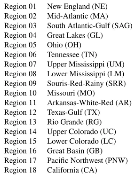
Table 1.List of USGS water-resources regions.
Region 01 New England (NE) Region 02 Mid-Atlantic (MA) Region 03 South Atlantic-Gulf (SAG) Region 04 Great Lakes (GL) Region 05 Ohio (OH) Region 06 Tennessee (TN) Region 07 Upper Mississippi (UM) Region 08 Lower Mississippi (LM) Region 09 Souris-Red-Rainy (SRR) Region 10 Missouri (MO)
Region 11 Arkansas-White-Red (AR) Region 12 Texas-Gulf (TX)
Region 13 Rio Grande (RG) Region 14 Upper Colorado (UC) Region 15 Lower Colorado (LC) Region 16 Great Basin (GB) Region 17 Pacific Northwest (PNW) Region 18 California (CA)
forecast skill across the entire CONUS for forecast lead times up to 6 months. Specifically, we seek in this study (1) to quantify the contributions of IHCs and FS to seasonal predic-tion of cumulative runoff (CR) and SM during each month of the year, and (2) to identify the months and sub-regions within CONUS, where improvement in simulating the IHCs and/or FS can have the greatest impact on seasonal hydro-logic forecast skill.
2 Approach
We conducted paired ESP and reverse-ESP experiments to generate forecasts with up to 6 months lead time (i.e. up to 6 months beyond the forecast initialization date) for the 33 yr reforecast period 1971–2003 over the CONUS. In ESP, an LSM is run using observed forcings up to the forecast initial-ization date to generate the IHC. During the forecast period, an ensemble of forcings is created from the time series of observations (gridded over the model domain, sampled from nhistorical years) starting on the forecast initialization date, and proceeding through the end of the forecast period (up to 6 months from the forecast initialization date for this analy-sis), for each ofnhistorical years. In reverse-ESP, the IHCs on the forecast date are taken from each of then historical years of simulation, but during the forecast period, the model is forced with the gridded observations for that year (essen-tially a perfect climate forecast).
We used the Variable Infiltration Capacity (VIC) model; a macroscale hydrology model (Liang et al., 1994; Cherkauer et al., 2003) that has been extensively used over the CONUS and globally (e.g. Maurer et al., 2001; Nijssen et al., 2001; Adam et al., 2007; Wang et al., 2009). VIC was applied over the CONUS at a spatial resolution of1/2degree latitude and
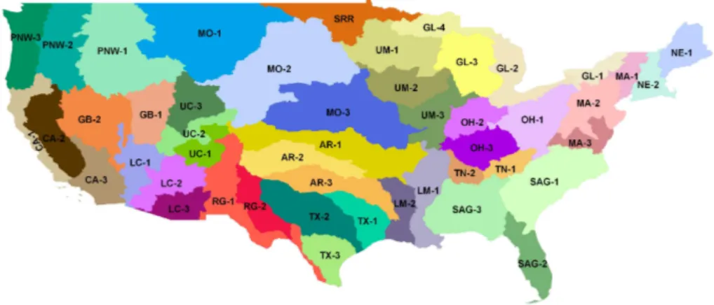
longitude. We then spatially aggregated the forecasts gener-ated by each experiment to the scale of 48 hydrologic sub-regions across the CONUS (Table 1 and Fig. 1). These 48 sub-regions were created by merging the 221 US Geological Survey (USGS) hydrologic sub-regions. Each sub-region is named after the water resources region in which it is located (Table 1). We compared the spatially aggregated forecasted cumulative runoff (CR) and mean monthly SM with the cor-responding observations (Sect. 2.2) for each sub-region and lead time over the reforecast period. We then estimated a forecast evaluation score (Sect. 2.4) and quantified the con-tributions of the IHCs and FS to seasonal hydrologic forecast skill.
2.1 Model implementation
The VIC model parameterizes the major surface, sub-surface, and land-atmosphere hydrometeorological processes and represents the role of sub-grid spatial heterogeneity in SM, topography, and vegetation on runoff generation (Liang et al., 1994). We ran the model in water balance mode, in which the moisture budget is balanced at a daily time step and model’s surface temperature is assumed to equal surface air temperature for purposes of energy flux computations (e.g., those associated with evapotranspiration and snowmelt). The model was run at a daily time step, except for the snow accu-mulation and ablation algorithm, which was run at a 3 h time step. The1/2degree parameters (i.e. vegetation, soils, ele-vation and snow band parameters) used in this study are the same as in Andreadis et al. (2005), which were aggregated from the North America Land Data Assimilation System pa-rameters used in Maurer et al. (2002). The three VIC soil layers had typical depths of∼0.10 m for the first layer, 0.2 to 2.3 m for the second layer, and 0.1 to 2.5 m for the third layer. Additional details of the model setup are included in Maurer et al. (2002) and Andreadis et al. (2005).
2.2 Synthetic truth data set
Fig. 1.48 hydrologic sub-regions of the CONUS as used in this study, based on aggregation of 221 USGS sub-regions.
from daily temperature and temperature range as in Maurer et al. (2002). We first ran the model for the period 1916–1969 starting from a prescribed initial state and saved the IHCs at the end of the simulation. Using those IHCs, generated after 53 yr of spin-up, we initialized the control run simu-lation over 1970–2003. The same IHCs were also used for generating IHCs for the 1st day of each month during each year of the reforecast period (1971–2003). We aggregated the model’s CR (i.e. sum of surface runoff and baseflow) and SM (i.e. sum of soil moisture of all three layers) to monthly values and spatially aggregated them to the 48 hydrologic sub-regions. These model-derived values served in lieu of direct observations for the purposes of our analyses. Maurer et al. (2002) and others have shown that when the VIC model is forced with high quality observations, it is able to repro-duce SM and streamflow well across the CONUS domain.
2.3 ESP and reverse-ESP implementation
In our implementation of ESP, we obtained the IHCs from a control run simulation (Sect. 2.2). Given the IHCs on the first day of each month from 1971–2003, we then forced the model with 31 ensemble members of observed (gridded) forcings (sampled from 1971–2001) starting on the forecast date for a period of six months. For example, to start the forecast on 01/01 (i.e. 1 January) of any yeari, we used IHC at the 00:00 h of the dayi/01/01 and ran the model with forc-ings fromj/01/01 toj/07/01 of each yearj between 1971– 2001. Figure 2b shows a schematic of the experimental de-sign where “true” IHCs were used to initialize the model and it was forced with resampled gridded observations.
The reverse-ESP experiments sampled 31 IHCs from the retrospective IHCs for each forecast initialization date (day 1 of each month) from 1971–2001. For example, to start the forecast on 01/01 of any yeari, we used IHC at the 00:00 h of the dayj/01/01 of each yearj between 1971–2001, and forced the model with gridded observations for the period i/01/01 toi/07/01. As shown in Fig. 2c, in the reverse-ESP
Fig. 2. Schematic diagram of(a)Observational analysis(b)ESP and(c)reverse-ESP.
experiment climatological IHCs (from the same simulation run used to extract the IHCs for the ESP runs) were used to initialize the model and it was forced with “true” observa-tions during the forecast period. CR and SM were computed as in the ESP experiment.
2.4 Forecast evaluation
Fig. 3. Variation of RMSE ratio (RMSEESP/RMSErevESP) with lead time over 48 hydrologic sub-regions, for the CR forecasts at lead 1–6 months, initialized on the beginning of the each month. (DJF: blue, MAM: green, JJA: light brown and SON: red).
timeκ. RMSEESPis then:
RMSEESP= v u u t
1 M
" M X
i=1 1 N
N X
j=1
Oik−Eij k 2
#
(1)
Likewise letRij kbe the CR or SM generated by the reverse-ESP experiment using the IHC of yearj and forcing of year iat a lead timeκso RMSErevESPcan be estimated by:
RMSErevESP= v u u t 1 M
"M X
i=1 1 N
N X
j=1
Oik−Rij k 2
#
(2)
We then calculated, the ratio of RMSE of each experiment (Eq. 3).
RMSE Ratio=RMSEESP/RMSErevESP (3)
Unless otherwise specified, we consider that if the ratio is less than 1 then IHCs dominate (in a relative sense) the sea-sonal hydrologic forecast skill and if it is greater than one then FS dominates.
2.5 κ parameter
Mahanama et al. (2011) introduced a parameter,κ, which is a ratio of the standard deviation of the initial SM+SWE (σw) to the precipitation during the forecast period (σP) (Eq. 4). Highκ values correspond to high total moisture variability at the time of forecast initialization relative to precipitation variability during the forecast period and vice versa. κ is basically a measure of the hydrologic predictability derived solely from knowledge of the IHCs at the start of the forecast period.
κ=σw/σP (4)
3 Results
In this section we examine the variation of relative contribu-tions of the IHCs and FS in the CR and SM forecast with each forecast initialization date (i.e. day 1 of each month) for lead times of 1 to 6 months across the CONUS. We also highlight the sub-regions and forecast periods for which improvement in knowledge of IHCs or FS would most improve seasonal hydrologic forecast skill.
3.1 Cumulative runoff forecasts
The variation of RMSE ratio for the forecast of CR at lead 1 to 6 months for each of the 48 hydrologic sub-regions is shown in Fig. 3; where CR at lead-1 [lead-6] is the CR over the first month [1 to 6 months] of the forecast period. RMSE ratios below 1.0 indicate that the relative forecast error due to uncertainties in the FS is lower than the error due to un-certainties in the IHCs; which indicates the relatively high contribution of the IHCs in the CR forecasts skill.
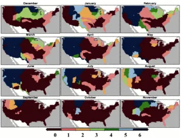
Fig. 4.Plot of the maximum lead (in months) at which RMSE Ratio is less than 1, for CR forecasts, initialized on the beginning of each month.
suggests that runoff forecasts in the above-mentioned sub-regions and forecast periods could benefit substantially from improvements in knowledge of the IHCs. For sub-regions in the Eastern US such as NE, MA, SAG-1 and -2, OH-1 and -2, and UM, RMSE ratios are less than one for lead 1–2 months, for CR forecasts initialized during win-ter – (December-January-February (DJF) – and spring month (March and April, mainly). This finding is in agreement with Li et al. (2009) who noted that the IHCs dominate the stream-flow (and SM) forecasts made during January and July, over Ohio and Southeastern US sub-regions, up to lead 1 month. These sub-regions as well could potentially benefit from im-provements in estimates of the IHCs during these seasons. Aside from those months and locations, FS dominates the CR forecasts. Some sub-regions such as TN, LM, and SAG-3 stand out because their RMSE ratios throughout the entire year and for all lead times exceeds 1, which suggests that in those sub-regions improved hydrologic forecasts must, for the most part, await improvements in FS.
There is also a clear difference between the variations of RMSE ratio initialized from wet vs dry IHCs. For example, in most sub-regions across the CONUS, forecasts initialized during summer months have RMSE ratios less than or equal to 1 for lead-1 month CR forecasts (also shown by Wood and Lettenmaier, 2008 and Li et al., 2009) for forecasts initial-ized during summer months. Furthermore the rate of change in the RMSE ratio for 1-month vs. 6-month forecasts is much higher in forecasts initialized in the summer months than in winter and spring months when the IHCs are generally wet. This property is particularly significant for predictions dur-ing droughts when the IHCs are dry. It potentially means that during a drought event when the IHCs are dry, the sig-nal from the IHCs may dominate even at lags for which the RMSE ratio exceeds 1. Additionally, in climatologically wet
periods followed by dry initial conditions, FS may well be important in improving seasonal hydrologic forecasts.
Figure 4 shows the maximum lead time (in months) at which the RMSE ratio of CR forecasts is below 1; defining the maximum lead time the IHCs can play a significant role in CR forecasts relative to FS. Beyond this lead, FS dom-inates the CR forecast skill; hence improvement in the FS would lead to higher forecast skill. For the most part, the sub-regions in Northeastern and Southeastern US would ben-efit most from improvements in FS throughout the year be-cause the IHCs dominate up to lead-2 only. In the mountain-ous west and Pacific Coast sub-regions FS dominates mainly during fall and winter. On the other hand, IHCs dominate in those sub-regions during spring and summer for up to 6 months lead time. GL, SRR, and UM sub-regions over-all would benefit most from improvement in knowledge of IHCs during winter and spring months (mainly March) and FS during summer months.
3.2 Soil moisture forecasts
SM is a key hydrologic state variable, and a natural indicator of agricultural drought. Figure 5 show the RMSE ratios of the mean monthly SM forecast, at lead-1 (i.e. mean monthly SM of the first month) to 6 (i.e. mean monthly SM of the 6th month of the forecast period) for forecasts initialized on the beginning of each month. In contrast to forecasts of CR, the RMSE ratio at lead-1 is almost always less than 1, across the CONUS and for each forecast period, indicating the strong dominance of IHCs for short lead forecasts. The ratio in-creases for leads greater than 1.
In the NE, MA, SAG, OH, LM, and TN sub-regions the in-fluence of IHCs beyond lead-1 is generally negligible, which in turn means that improvement in FS will be required to improve SM forecasts beyond lead-1. This pattern for SM forecasts was also shown by Li et al. (2009) in the Ohio and southeastern regions. Conversely, in the majority of the sub-regions in the Midwestern US, such as GL-1, -2, -3; SRR, UM, and the Western US show strong IHC influence for SM forecasts up to lead-5, when the forecast is initialized in win-ter or spring months. In snowmelt-dominated sub-regions in the Western US, the skill of SM forecasts during spring and summer months is especially high. In UC, LC, PNW, GB, and CA sub-regions, useful skill in SM forecasts can be derived from the IHCs for leads as long as 6 months for forecasts initialized during the summer months.
Overall, the relative contributions of IHCs are greater for forecasts of SM than for forecasts of CR at lead-1 month. The contribution of IHCs is dominant over the Western US, in particular during spring and summer months.
Fig. 5.Variation of RMSE ratio (i.e. RMSEESP/RMSErevESP) with lead time over 48 hydrologic sub-regions, for the SM forecasts at lead-1
to 6 months, initialized on the beginning of the each month. (DJF: blue, MAM: green, JJA: light brown and SON: red).
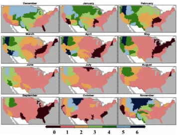
Fig. 6.Plot of the maximum lead (in months) at which RMSE Ratio is less than 1, for mean monthly SM forecasts, initialized on the beginning of each month.
Northeastern and Southeastern US). This means that the rela-tive contribution of the IHCs in the SM forecasts is more ex-tensive than in the CR forecasts during the first month of the forecast period (i.e. lead-1). The spatial contrast between the sub-regions and forecast periods with high and low values of maximum lead time, where IHCs significantly influence the SM forecasts skill, is similar to CR forecasts.
3.3 Controls on hydrologic forecast skill
Mahanama et al. (2011) found a first order relationship be-tween IHC-based 3-month streamflow forecasts (that is, fore-casts wherein CR was regressed on the IHCs) andκ. Fol-lowing their analogy we expect a first order relationship
be-tween the inverse RMSE ratio (i.e. RMSErevESP/RMSEESP) andκ. Namely, we expect that RMSEESPshould be smaller for sub-regions and forecast periods with higherκ. Scatter of the inverse RMSE ratio andκare shown for forecast periods of 1, 3, and 6 months in Fig. 7a–c, respectively. Red cir-cles and blue circir-cles show the inverse RMSE ratio estimated across all the hydrologic sub-regions and forecast initializa-tion dates for the forecast of CR and mean monthly SM at lead-1, lead-3, and lead-6 (Fig. 7a–c, respectively). The val-ues ofκ vary for different forecast periods, and in general, the number of hydrologic sub-regions and forecast periods withk >1 decreases as the lead time increases. First order relationships between the inverse RMSE ratio andκ clearly exist at each lead time. The range of inverse RMSE ratios for a givenκ value seems to be higher for CR at lead-1 than for SM (Fig. 7a). Overall at lead-1, the inverse RMSE ratio is higher for SM than for CR. The values of the inverse RMSE ratio of SM and CR forecast is much more comparable in lead-3 forecast (Fig. 7b). The inverse RMSE ratio for lead-6, CR forecast is generally higher than its corresponding values for SM forecasts at lead-6 (Fig. 7c).
4 Summary and conclusions
Fig. 7. Inverse RMSE ratio (i.e. RMSErevESP/RMSEESP) of CR and mean monthly SM forecasts at(a)lead-1(b) lead-3, and(c)
lead-6 plotted againstκparameter of each forecast period (i.e. 1 month, 3 months, and 6 months, respectively).
can benefit most from improvements in the FS or knowledge of the IHCs. Our key findings are:
1. IHCs generally have the strongest influence over CR and SM forecasts at lead-1, beyond which their influ-ence decays at rates that depend on location, lead time, and forecast initialization date.
2. Beyond lead-1, IHCs primarily influence the CR and SM forecasts during spring and summer months, mostly over the Western US.
3. FS dominates CR and SM forecast skill beyond lead-1 mainly over the Northeastern and Southeastern US throughout the year. For the rest of the CONUS, FS generally dominates CR and SM forecasts during fall and early winter months.
4. The relative contributions of IHCs and FS have a first order relationship with the ratio of initial total moisture variability to the variability of precipitation during the forecast period for the temporal scale of seasonal hy-drologic prediction.
While the ESP-based framework used in this study allows a consistent estimation of the contribution of the IHCs and FS over large spatial scale (e.g. continental scale) and long time period, it is important to understand the limitations of
the study design. The distribution of FS (in the ESP exper-iment) and IHCs (in the reverse-ESP experexper-iment) is uncon-ditional (i.e. climatological distribution) and we assume that IHCs (in the ESP experiment) and FS (in the reverse-ESP ex-periment) are perfect, hence our results arguably provide an upper bound on the contributions of the IHCs and FS to sea-sonal hydrologic prediction skill. Furthermore since we do not route the runoff through the stream network and rather use spatially aggregated values, there will be some differ-ence in the spatial extent and lead time of the contribution of IHCs (mainly snow-melt) in streamflow based on the time of concentration of a given basin, although this effect can be expected to be limited, for the most part, to about a month.
We believe the findings of this study could have impor-tant implications for the improvement of seasonal hydro-logic and drought prediction in the CONUS. We identified the sub-regions and forecast periods during which improve-ment in the knowledge of IHCs and FS could result in the most improvement in seasonal hydrologic prediction skill. For those river basins and forecast periods which have a sub-stantial contribution of IHCs to seasonal hydrologic predic-tion skill, for instance, skill improvements might be derived by improving the IHCs – for example through the assimila-tion of ground based or remote sensing data. Another pos-sible way of improving seasonal hydrologic forecasts with relatively short leads may be to exploit the skill of medium range weather forecasts over the first 1–2 weeks of the fore-cast period.
Appendix A
Abbreviations used
AR Arkansas-White-Red CA California
FS Climate Forecast Skill CONUS Conterminous United States CR Cumulative Runoff
DJF December-January-February ESP Ensemble Streamflow Prediction
GB Great Basin
GL Great Lakes
IHC Initial Hydrologic Conditions JJA June-July-August
LC Lower Colorado LM Lower Mississippi LSM Land Surface Model MA Mid-Atlantic MAM March-April-May
MO Missouri
NE New England
OH Ohio
RG Rio Grande
RMSE Root Mean Square Error SAG South Atlantic-Gulf SM Soil Moisture
SON September-October-November SRR Souris-Red-Rainy
SWE Snow Water Equivalent SWM Surface Water Monitor
TN Tennessee
TX Texas-Gulf UC Upper Colorado UM Upper Mississippi
USGS United States Geological Survey VIC Variable Infiltration Capacity
Acknowledgements. We thank Elizabeth Clark, Ben Livneh and Mohammad Safeeq for their valuable comments and suggestions on earlier versions of this paper. This research was supported in part by the National Oceanic and Atmospheric Administration (NOAA) grants No. NA08OAR4320899 and NA08OAR4310210 to the University of Washington.
Edited by: J. Seibert
References
Adam, J. C., Haddeland, I., Su, F. and Lettenmaier, D. P.: Simu-lation of reservoir influences on annual and seasonal streamflow changes for the Lena, Yenisei, and Ob’rivers, J. Geophys. Res., 112, D24114, 2007.
Andreadis, K. and Lettenmaier, D.: Assimilating remotely sensed snow observations into a macroscale hydrology model, Adv. Wa-ter Resour., 29, 872–886, 2006.
Andreadis, K. M., Clark, E. A., Wood, A. W., Hamlet, A. F. and Lettenmaier, D. P.: 20th century drought in the conterminous United States, J. Hydrometeorol., 6, 985–1001, 2005.
Cherkauer, K. A., Bowling, L. C., and Lettenmaier, D. P.: Vari-able infiltration capacity cold land process model updates, Global Planet Change, 38, 151–159, 2003.
Clark, M. P., Slater, A. G., Barrett, A. P., Hay, L. E., McCabe, G. J., Rajagopalan, B., and Leavesley, G. H.: Assimilation of snow covered area information into hydrologic and landsurface mod-els, Adv. Water Resour., 29, 1209–1221, 2006.
Hayes, M., Svoboda, M., Le Comte, D., Redmond, K., and Pas-teris, P.: Drought monitoring:New tools for the 21st century, in: Drought and Water Crises: Science, Technology, and Manage-ment Issues, edited by: Wihite, D. A., Taylor and Francis, Boca Raton (LA), 53–69, 2005.
Kalnay, E. C., Kanamitsu, M., Kistler, R., Collins, W., Deaven, D., Gandin, L., Iredell, M., Saha,S., White, G., Woollen, J., Zhu, Y., Chelliah, M., Ebisuzaki, W., Higgins, W., Janowiak, J., Mo,K. C., Ropelewski, C., Wang, J., Leetmaa, A., Reynolds, R., Jenne, R., and Joseph, D.: The NCEP/NCAR 40 yr reanalysis project, B. Am. Meteorol. Soc., 77, 437–472, 1996.
Koster, R. D., Mahanama, S. P. P., Livneh, B., Lettenmaier, D. P., and Reichle, R. H.: Skill in streamflow forecasts derived from large-scale estimates of soil moisture and snow, Nat. Geosci., 3, 613–616, 2010.
Krishnamurti, T. N., Kishtawal, C. M., LaRow, T. E., Bachiochi, D. R., Zhang, Z., Williford, C. E., Gadgil, S., and Surendran, S.: Im-proved weather and seasonal climate forecasts from multimodel superensemble, Science, 285, 1548–1550, 1999.
Li, H., Luo, L., and Wood, E. F.: Seasonal hydrologic predictions of low-flow conditions over Eastern USA during the 2007 drought, Atmos. Sci. Lett., 9, 61–66, 2008.
Li, H., Luo, L., Wood, E. F., and Schaake, J.: The
role of initial conditions and forcing uncertainties in sea-sonal hydrologic forecasting, J. Geophys. Res., 114, D04114, doi:10.1029/2008JD010969, 2009.
Liang, X., Lettenmaier, D. P., Wood, E. F., and Burges, S. J.: A simple hydrologically based model of land surface water and en-ergy fluxes for general circulation models, J. Geophys. Res., 99, 14415–14428, 1994.
Luo, L. and Wood, E. F.: Monitoring and predicting
the 2007 US drought, Geophys. Res. Lett., 34, L22702, doi:10.1029/2007GL031673, 2007.
Mahanama, S. P., Livneh, B., Koster, R. D., Lettenmaier, D. P., and Reichle, R. H.: Soil Moisture, Snow, and Seasonal Streamflow Forecasts in the United States, e-View, doi:10.1175/JHM-D-11-046.1, 2011
Maurer, E. P. and Lettenmaier, D. P.: Predictability of seasonal runoff in the Mississippi River basin, J. Geophys. Res., 108, 8607, doi:10.1029/2002JD002555, 2003.
Maurer, E. P., Wood, A. W., Adam, J. C., Lettenmaier, D. P., and Nijssen, B.: A Long-Term Hydrologically Based Dataset of Land Surface Fluxes and States for the Conterminous United States, J. Climate, 15, 3237–3251, 2002.
Maurer, E. P., Lettenmaier, D. P., and Mantua, N. J.: Variability and potential sources of predictability of North American runoff, Water Resour. Res., 40, W09306, doi:10.1029/2003WR002789, 2004.
Maurer, E. P., O’Donnell, G. M., Lettenmaier, D. P. and Roads, J. O.: Evaluation of the land surface water bud-get in NCEP/NCAR and NCEP/DOE reanalyses using an off-line hydrologie model, J. Geophys. Res., 106, 17841–17862, doi:10.1029/2000JD900828, 2001.
McGuire, M., Wood, A. W., Hamlet, A. F., and Lettenmaier, D. P.: Use of satellite data for streamflow and reservoir storage fore-casts in the Snake River Basin, J. Water Res. Pl.-ASCE, 132, 97, 2006.
Nijssen, B., O’Donnell, G. M., Hamlet, A. F. and Lettenmaier, D. P.: Hydrologic sensitivity of global rivers to climate change, Cli-matic Change, 50, 143–175, 2001.
Stefanova, L. and Krishnamurti, T. N.: Interpretation of Seasonal Climate Forecast Using Brier Skill Score, The Florida State Uni-versity Superensemble, and the AMIP-I Dataset, J. Climate, 15, 537–544, 2002.
Svoboda, M., LeComte, D., Hayes, M., Heim, R., Gleason, K., Angel, J., Rippey, B., Tinker, R., Palecki, M., Stooksbury, D., Miskus, D., and Stephens, S.: The Drought Monitor, B. Am. Meteor. Soc., 83, 1181–1190, 2002.
Tang, Q., Wood, A. W., and Lettenmaier, D. P.: Real-Time Precipi-tation Estimation Based on Index SPrecipi-tation Percentiles, J. Hydrom-eteorol., 10, 266–277, doi:10.1175/2008JHM1017.1, 2009. Wang, A., Bohn, T. J., Mahanama, S. P., Koster, R. D. and
doi:10.1175/2008JCLI2586.1, 2009.
Wood, A. W.: The University of Washington Surface Water Mon-itor: An experimental platform for national hydrologic assess-ment and prediction, in Proceedings AMS 22nd Conference on Hydrology, New Orleans, LA, 20–24 January 2008, 2008. Wood, A. W. and Lettenmaier, D. P.: A test bed for new seasonal
hydrologic forecasting approaches in the Western United States, B. Am. Meteorol. Soc., 87, 1699–1712, 2006.
Wood, A. W. and Lettenmaier, D. P.: An ensemble approach for attribution of hydrologic prediction uncertainty, Geophys. Res. Lett., 35, L14401, doi:10.1029/2008GL034648, 2008.