Maio de 2015
Working
Paper
388
Fiscal interactions and spillover effects of
a federal grant to Brazilian municipalities
TEXTO PARA DISCUSSÃO 388•MAIO DE 2015• 1
Os artigos dos Textos para Discussão da Escola de Economia de São Paulo da Fundação Getulio
Vargas são de inteira responsabilidade dos autores e não refletem necessariamente a opinião da
FGV-EESP. É permitida a reprodução total ou parcial dos artigos, desde que creditada a fonte.
Escola de Economia de São Paulo da Fundação Getulio Vargas FGV-EESP
Fiscal interactions and spillover effects of a federal grant to
Brazilian municipalities
Marcelo Castro∗ Enlinson Mattos† Rebeca Regatieri‡ May, 2015
Abstract
What is the impact of an unconditional transfer to a municipality when the municipality’s neighbor also receives the transfer? In this paper, we test whether a federal government grant, the Municipalities’ Participation Fund (Fundo de Participa¸c˜ao dos Munic´ıpios - FPM), differently affects municipal expenditures depending on neighbor cities. We use cities near one of the four points of discontinuity in the FPM transfers according to population brackets and with neighbors near different thresholds. We estimate the impacts of own and neighbor FPM using the method of Regression Discontinuity Design (RDD). The results indicate that part of the flypaper effect of FPM on local economies that has been estimated in the literature can be explained by increased spending in neighboring municipalities. The spillover is generally positive, with the exception of spending on health and sanitation in some population groups. We also consider a sample of neighbors that are more distant from the thresholds, and we show that in these cases the differences on estimations when we control for the neighbors’ FPM are not substantial. Ultimately, we find an effect on the neighbor populations that helps clarify the observed FPM correlation in neighboring municipalities.
Keywords: fiscal federalism, program evaluation, flypaper effect, fiscal spillover.
Resumo
Qual o impacto de uma transferˆencia incondicional a um munic´ıpio quando seu vizinho tamb´em recebe a transferˆencia? Nesse artigo n´os testamos se uma transferˆencia do governo federal, o Fundo de Participa¸c˜ao dos Munic´ıpios (FPM), afeta os gastos municipais de forma diferente dependendo dos munic´ıpios vizinhos. N´os utilizamos munic´ıpios pr´oximos a um dos quatro pontos de descontinuidade no repasse do FPM de acordo com faixas de popula¸c˜ao e que possu´ıam vizinhos pr´oximos a pontos de descontinuidade diferentes. N´os estimamos o impacto do FPM recebido pelo pr´oprio munic´ıpio e pelo vizinho usando o m´etodo de Regress˜oes em Descontinuidade (RDD). Os resultados indicam que parte do efeito flypaper do FPM sobre a economia local estimado na literatura pode ser explicado pelo aumento de gastos nos munic´ıpios vizinhos. O spillover ´e em geral positivo, com exce¸c˜ao dos gastos em sa´ude e saneamento em algumas faixas populacionais. N´os tamb´em consideramos uma amostra de vizinhos mais distantes dos pontos de descontinuidade, e mostramos que nesse caso as diferen¸cas nas estimativas quando controlamos pelo FPM do vizinho n˜ao s˜ao substanciais. Por ´ultimo, encontramos um efeito positivo do FPM sobre a popula¸c˜ao dos munic´ıpios vizinhos, o que ajuda a esclarecer a correla¸c˜ao observada entre o FPM de cidades vizinhas.
∗Corresponding author. S˜ao Paulo School of Economics (EESP / FGV-SP). Email:
marceloac.econ@gmail.com.
†S˜ao Paulo School of Economics (EESP / FGV-SP). Email: Enlinson.mattos@fgv.br
‡Master in Economics at S˜ao Paulo School of Economics (EESP / FGV-SP) and Finance and Control Analyst
1
Introduction
In federalist economies, it is fundamental to investigate the extent of strategic interactions among jurisdictions to determine the distribution of government resources to subnational entities. In addition, fiscal spillovers help predict better tax and expenditure responsibilities in those jurisdictions. Although a large body of empirical literature has emerged in recent years that has documented the existence of fiscal spillovers, such studies generally lack identification issues in their estimation.
The aim of this article is to identify the causal effect of a federal grant to a municipality on its own expenditures, separating from the effect of neighbors’ grants, the grant spillover effect. We consider an unconditional and involuntary transfer rule from the federal government to Brazilian municipalities, the Participation Fund of Municipalities (Fundo de Participa¸c˜ao dos Munic´ıpos - FPM), as a source of exogenous variation in local spending. FPM grants are distributed according to well-defined population brackets, thereby allowing us to use municipalities that are close to discontinuity thresholds to identify exogenous variation in the transfers to those jurisdictions. The method of Regression Discontinuity Design (RDD) allows us to work around a central problem in the empirical literature, the endogeneity of neighbors’ fiscal responses.
near the thresholds. Thus, we consider cities with similar populations, some of which receive a large amount of additional federal funds because of small increases in population beyond the thresholds.
In theoretical terms, there are three general ways in which a city’s expenses could spill over onto its neighbors (Wilson, 1999). When the number of jurisdictions is small, the local taxes are chosen in strategic fashion, taking into account the inverse relationship between a jurisdiction’s tax rate and its base. A related body of literature focuses on welfare competition, specifically on income redistribution by local governments when the poor migrate in response to differing welfare benefits. A third body of literature analyzes the strategic interactions caused by benefit spillovers. However, according to Brueckner (2000), these theoretical models can be classified into two main categories: spillover models and resource-flow models. The former category incorporates cases in which local public expenditures can be correlated among neighbors when a good’s production can be exploited by people from neighboring municipalities, as with highway construction, environmental models, and efforts to reduce crime. The latter category includes tax and welfare competition models as well as the yardstick competition model (Besley and Case, 1995), in which voters can observe and compare the taxes and public service delivery in neighboring municipalities before legitimize mayors’ second terms.
Our results confirm the existence of the spillover effect, in contrast to the most recent findings by Isen (2014), that found no significant fiscal spillover effect for a sample of American counties, municipalities and school districts. More importantly, our estimation suggests a larger spillover effect than those previously found in the literature, and our identification strategy allows to control for the neighbor’s fiscal policy variation to estimate the local response to federal grant. We find a reduction in the flypaper estimates compared with those found in the literature.
2
Data and institutional background
FPM grants are the federal government’s most important transfer to municipalities and the main revenue sources of small municipalities. In our sample, FPM grants account for an average of 45% of local budget revenues, which comprise tax revenues and transfers. The fund was created in the 1947 Constitution, but the rule’s actual legal basis is outlined in the 1988 Constitution, from Article 159 on, which sets the rule for allocating the fund’s resources. Article 160 of the Constitution prohibits any constraints on the destination of these resources and restricts the possibility of conditioning the transfer itself.
Transferring the FPM grants by population bracket was first established in 1966 with Law No. 5,172 and the Complementary Act 35 of 1967, and the current thresholds were defined in the 1981 Decree Law No. 1,881, approved by Legislative Decree 19 of 1982. Complementary Law No. 59 of 1988 determined that FPM population coefficients should be reviewed annually according to population estimates released by the National Statistics Institute (Instituto Brasileiro de Geografia e Estat´ıstica - IBGE). Complementary Law No. 62, from 1989, postponed this change, as did successive laws, such that this transition was only completed in 2007. Complementary Law No. 62 also defined the Court of Audit (Tribunal de Contas da Uni˜ao - TCU) as the responsible body for monitoring and calculating the coefficients and creating additional legislation to regulate the infra-constitutional background.
During the initial years of the 1990s, the transfers were still made based on 1981 decree law coefficients. Beginning in 1993, the 1991 Census population was considered for cities that were created after this census. Complementary Law No. 91 from 1997 determined the convergence of the annual FPM grants to municipalities based on previous year population estimated by IBGE over a transition period of four years, that was subsequently extended until 2007. This transition aimed to help cities avoid drastically reductions in budget revenues, especially for cities that had lost population because of migration or emancipation. In these cases, the annual extra FPM, compared with the values under the 1995 coefficients, was discounted annually until 2007 (TCU Normative Decision No. 14, 1996).
directly by the municipalities. We separately analyze the main municipal expenditures according to the function in public administration: health, education, urbanization and basic sanitation1. Nominal values (in reais, R$) were updated to January 2014 using the official Consumer Price Index (´Indice de Pre¸cos ao Consumidor Amplo - IPCA), calculated by IBGE2. Additionally, we
use information about local populations estimates released by IBGE.
The preparation of FINBRA stems from Law No. 4,320, from 1964, Articles 111 and 112, and Complementary Law No. 101, from 2000, Article 51. Each municipality sends the Table of Consolidated Municipal Financial Data to a public national bank, and the National Treasury compiles the information. We have an unbalanced panel with approximately 4,000 municipalities that had fewer than 30,000 inhabitants between 2002 and 2012. There is an attrition rate of approximately 5% caused by municipalities that did not send their information in different years, generally, small towns with fewer than 10,000 inhabitants.
The data regarding local populations derive from population censuses that were conducted every ten years by the IBGE and the census population counts conducted at halftime. In the period considered, there were population censuses in 2000 and 2010 and a population count in 2007, that are used to FPM distribution during the period 2003-2012. In the period between population censuses, IBGE provides population estimates calculated from the growth rates between the previous two censuses, weighted by country and state growth (IBGE, 2008). IBGE publishes annual estimates until August 31 of each year, and by October 31, the final estimates are sent to TCU (Article 102, Law No. 8443 of July 16, 1992). These estimates refer to July 1 of each year (t) and are used to calculate FPM transfers in the following year (t + 1) (Minist´erio da Fazenda, 2005; 2012a).
We calculate the amounts that should have been transferred in accordance with the law, which we call theoretical FPM, to determine whether the values reported to FINBRA by the mayors are correct3. Now, we explain the calculation of the financial reducer to the period 2002-2007. First, we define the Additional Gain (AGit), a an auxiliary variable, for each
municipality as the difference between the tabulated population coefficient in 1995 and the coefficient of the previous year, t-1:
1Considering the municipalities in our sample, the main types of expenditures in each function are: health
-primary care and hospital assistance; education - elementary and childhood education; urbanization - construction of roads and public works; sanitation - urban sanitation. More information about this expenditure classification is available in Rezende (2007).
2
US$1 was approximately equal to R$2.35 during this period at the official exchange rate.
3
AGit=k(popi,1995)−k(popi,t−1) ifAGit>0 ; 0 otherwise
Where k is the coefficient of population used as a source of exogenous variation on FPM transfer in our sample of cities. In fact, k is a step function of previous year local population estimated by IBGE and tabulated by the law, as shown in Table 1 of appendix E.
There is a percentual reduction in (AGit), 1−Rt, whereRtis defined by law and increases
along the years, in such a way that there is a convergence of all cities by 20084. We use the variable Additional Adjusted Gain,AAGit:
AAGit=AGit×(1−Rt) ifAGit>0 ; 0 otherwise
We define the Non-Supported Cities Coefficient,N SCit, as:
N SCit =k(popi,t−1) if AGit≤0 ; 0 otherwise
The percentage, Rt, that is not used for cities which coefficients decreased is redistributed
to the Non Supported Cities. The total Share to Redistribute,SRit,can be written as:
SRit=
Σj,t,SAGjt−Σj,t,SAAGjt
Σj,t,SN SCjt
×N SCit ifAGit ≤0 ; 0 otherwise
That is, SR is the value reduced from cities that receive additional gain (AG >0) that are distributed each city that are not supported by additional gain (AG ≤ 0), according to the weight of each non supported city given all cities in the same situation in a given state and year. The Final City Coefficient, F Cit, is defined as:
F Cit=k(popi,t−1) +AAGit ifAGit>0 and year ≤2007
F Cit=k(popi,t−1) +SRit ifAGit≤0 and year ≤2007
F Cit =k(popi,t−1) if year>2007
Finally, theoretical FPM can be described by Equation (1):
theoreticalF P Mit=
F Cit
Σj|SF Cjt
×ei×Mt×0.864 (1)
We divide the final coefficient of each city, FC, which is a direct function of the previous year’s population coefficient, for the state total. Then, we multiply this percentage by the total destined to city i’s state,ei, which follows a tabulation defined by the FPM law (TCU Resolution
4Financial reducer (R
242/1990) and presented in Table 2 of Appendix E.Mt´e the national amount allocated to the
FPM each year, determined as 23.5% of the income tax and the tax on industrialized products collected by the union. 86.4% of this amount is destined for interior cities with fewer than 140,000 inhabitants, which applies to all the cities in our sample.
We calculate in Equation (2) the increase in the theoretical FPM due to the previous year population variation, for the period 2008-2012:
∆theoreticalF P Mit
∆popi,t−1
= ∆kit(∆popi,t−1)Σj=6 i|Skjt(popj,t−1) (Σj|Skjt(popj,t−1))2
×ei×Mt×0.864 (2)
The effect of population growth on theoretical FPM is heterogeneous among cities because FPM distribution for interior cities also depends on the state. This effect is positive when the population grows beyond the FPM thresholds, but it is decreasing because the coefficient variation between the brackets is always the same (as shown in Table 1 of Appendix E). The derivatives for supported and non supported cities during the years that the reducer was applied follow a similar pattern.
3
Empirical strategy
We want to analyze the effect of extra FPM transfers received by municipalities on their budget expenditures considering the spillover effects from neighboring cities, which could also have received extra transfers. An Ordinary Least Squares (OLS) regression using all cities would likely be spurious given that per capita local spending and FPM are both correlated with local population. Also, similar neighboring municipalities are affected by similar cost shocks to local public goods provision and prices as well as by national trends in the economy, situations that could wrongly suggest a spillover effect (Revelli, 2005).
The methodology commonly used to estimate causal FPM impacts is based on this grant distribution law, which determines that part of the amount is transferred according to specific population segments. Hence, causal identification relies on the assumption that per capita FPM variation can be considered a random experiment near the thresholds. There is a small or null probability that a municipality receives a different value from the one established by this legal criterion of city population, because the transfers are automatically made monthly following accounting rules of apportionment.
local characteristics that are correlated with local spending to ensure causal impacts identification (Lee, Lemieux, 2010), for example, political-administrative conditions and voters’ preferences for public goods. This means that the population brackets that are used to transfer funds to cities cannot be correlated with other factors that influence local expenditures, at least in small regions near the thresholds. Additionally, the method implies that it is not possible to complete manipulate population, what could result in nonrandom variation between control and treatment groups, but we do allow for some non-prohibitive marginal manipulation.
Many papers have used this methodology and have found a positive impact of FPM on local expenditures (for example, Arvate et al, 2013, and Castro and Regatieri, 2014). In this paper, we argue that part of the estimated FPM effect on local expenditures may occur because of spillover effects from the FPM grants that were transferred to neighbor municipalities. The correlation between the population growth in neighboring municipalities leads to correlations among received FPM, even if we control for local fixed effects. Thus, we show that the FPM impact estimated by RDD are sensitive to the choice of neighbor cities.
There are three types of spillover or spatial interactions due to FPM that we are concerned. First, the estimated impact using FPM population rule ignores general equilibrium effects caused by the transfer. In particular, the estimated effect is the result of fiscal interactions between municipalities that receive the resource and their neighbors. Additionally, depending on the complementarity of neighbors’ spending, prices and demand can be impacted. General equilibrium effects are difficult to distinguish, but their presence does not invalidate the estimates if our interest is on the final effect of the experiment.
and neighbors j are necessarily in either the treatment or the control groups at any of the other thresholds.
Finally, the third and more challenging possibility of spillover occurs even when we control for city i and neigbor j at different thresholds. Municipalities that surpass one threshold during the period may probably have neighbors that also surpass different thresholds because of the population growth correlation of neighboring municipalities. The formula for the annual population growth estimated by the IBGE, as will be made clear in Section 4, depends on the growth in each city, region and country, between the two previous censuses. This generates treatment correlation among neighbors that are close to different thresholds. We control for this type of spillover adding the cities i and j’s FPM grants simultaneously in the regressions.
Our empirical strategy finds support in the empirical literature that seeks to estimate the spillover effect of social experiments. For example, Acemoglu and Angrist (2000) use two endogenous variables to estimate school peer effects. They control for student’s measured ability, as for the school mean ability, as there is a common thought that students’ abilities are correlated within a school. There is a literature that also considered double randomization as the best way to estimate spillover effect (Angelucci, De Giorgi, 2009; Angelucci, Di March, 2010). Thus, we simultaneously control for own and neighbor j’s populations as two different instruments, possibly correlated, to identify a own and neighbor’s FPM effects, as it equivalent to take random cities i that are eligible for the treatment and then randomize their neighbors j. We detail our strategy considering cities i and j with populationspi andpj in small windows
around different thresholds with no intersection among them. We consider for now 2 population thresholds (we use four thresholds in our estimates), p1 and p2, and that F P Mi is a function
of p1 and F P Mj is a function of p2, as the only variable considered affecting FPM transfers
E(Gi|Ti, Tj, pi, pj) =g0(pi) + [g1(pi)−g0(pi)]Ti+w0(pj) + [w1(pj)−w0(pj)]Tj
where
Ti = 1(pi ≥p1)
and
Tj = 1(pj ≥p2)
Gi is city i’s spending, which depends on its population and that of its neighbor. Ti is a
binary treatment that indicates whether municipality i receives an additional transfer, which occurs when the population,pi, is greater than the cutoff,p1. g1(pi) is the potential expenditure
of municipalities with population pi because of a R$1 per capita of transfer, while g0(pi) is the
potential expenditures of these cities when the mayors do not have that additional income. The same is true forTj, which is 1 when the population of city j,pj, is bigger than a given threshold,
p2, withp16=p2. Also,w1(pj) is the potential spillover of city j onto city i spending when city j
receives the extra FPM grant andw0(pj) is the potential spillover of city j onto city i en when
city j does not receive the extra amount.
Thus, the total impact of the city i’s FPM grant on local spending is equal to the potential direct impact of receiving an extra money plus the additional spillover of neighbors receiving the extra money. The identification problem is that we do not observeg0 and g1 for the same municipality with population pi, in the same way that we do not observe w0 and w1 for the
same city with populationpj.
We consider that transfers follow a continuous distribution based on the population, except at the thresholds, and that potential expenditures g0 and g1 are continuous at p1 as w0 and w1 are continuous at p2. Theoretical identification of treatment effect using RDD relies on
the distribution limits of dependent and independent variables at the thresholds (Imbens and Lemieux, 2008). We define the Local Average Treatment Effect (LATE) as the effect of a marginal population variation near the thresholds on city i’s expenditures:
LAT Ei(p1) = lim
pi→(p1)+
E(Gi|Ti, Tj, pj)− lim pi→(p1)−
E(Gi|Ti, Tj, pj) =
lim
pi→(p1)+
E(Gi|Ti = 1, Tj, pj)− lim pi→(p1)−
g1(p1)−g0(p1) + (w1(pj)−w0(pj))[E(Tj|pi →p+1, pj)−E(Tj|pi →p−1, pj)] =
g1(p1)−g0(p1) + (w1(pj)−w0(pj))[P(pj > p2|pi→p+1)−P(pj ≤p2|pi →p−1)]
The causal effect of the city i’s FPM grant on own expenditures, g1(pi)−g0(pi), can be
consistently identified without considering spillover effects if there is no correlation between neighbor’s populations. In this case, the impact of F P Mi on city i’s expenditures could be
estimated by regressing expenditures on FPM transfers in a vicinity of the cutoffp1. Nonetheless,
the spillover effect is nonzero if there is correlation between neighbor’s populations:
P(pj > p2|pi →p+1)=6 P(pj ≤p2|pi→p−1)
In this case, not controlling for neighbor j’s FPM spillover biases the estimated treatment impact. There are arguments that support this possibility, as neighbor’s populations are correlated, because local population growth estimates are highly influenced by regional conditions (IBGE, 2008), as we explain in Section 4. Therefore, as we approximate the potential values exactly at the thresholds for observations close to them, the possibility of population correlation among neighbors should not be ignored. Estimates using fixed effects can also be biased because of the same source of correlation between neighbors’ population growth.
Again, the spillover identification problem is that we can not estimate w1 ew2 for the same city j. Again, we explore the FPM law discontinuities and we consider neighbors j around the population thresholds, in such a way that cities i and j are in different threshold windows. In the case of non-zero spillover effects, we can identify the total effect of the cities i and j’s FPM grants on i’s expenditures as:
LAT Eij(p1, p2) = lim
pj→(p2)+
LAT Ei− lim pj→(p2)−
LAT Ei
= (g1(p1)−g0(p1)) + (w1(p2)−w0(p2)) (3)
(2SLS) approach, but for only one endogenous variable. Indeed, RDD estimation can be consistently generated by 2SLS (Imbens and Lemieux, 2008; Angrist and Lavy, 1999). The first stage consists of regressing cities i and j’s declared FPM per capita on i and j’s theoretical FPM per capita, the calculated amount that should have been transferred strictly under the law. In the second stage we estimate the impacts of i and j’s FPM per capita predicted in the first stage on i’s budget expenditure. 2SLS estimates Intended To Treat effects, which means the average effect on the population of compliers (Angrist, Imbens and Rubin, 1996), but as there are no deviations from the rule, 2SLS regression estimates equation (3).
The first stage specification is:
F P M =λ0+λ1theoreticalF P M +λ2g2(p) +v (4)
where FPM is the vector of cities i and j’s declared per capita FPM and theoreticalFPM is the vector of cities i and j’s theoretical per capita FPM, g2(p) is the vector of i’s and j’s
population polynomials of order 2. The second stage regression is:
Gi =α0+τ F P M∗+α1g2(p) +ϑi (5)
where Gi is city i’s municipal budget expenditures and F P M∗ are the cities i and j’s FPM
per capita estimated in the first stage. τ is the vector of the coefficients of interest. ϑiis the city
i’s idiosyncratic error term, which we cluster by city i to control the variance of each city over time (Wooldrigde, 2002). We also estimate regressions using the variable logarithms, except for the populations terms. Estimation using panel data to control for local fixed effects guarantees the robustness of results as local population growth is a continuous function of population, in such a way that politicians can not manipulate population growth, as we demonstrate in Section 4.
The regression model that we present is a local linear regression, so that the results are valid only for the municipalities located near the thresholds5. Nevertheless, we analyze the effects at
different population thresholds - 10,188, 13,584, 16,980 and 23,772 inhabitants. This guarantees a degree of external validity for the average effect estimation in municipalities with up to 30,000 inhabitants, which account for approximately 80% of Brazilian municipalities and nearly 25%
5
of the national population.
The fact that the treatment variable is not binary suggests the use of a fuzzy RDD, which allows for the heterogeneity of treatment among the participants. The hypotheses of identification are the same as those used in the sharp design that have been presented so far. The complete discontinuity of the treatment variable is not strictly necessary for the RDD given that there is some exogenous variation in the treatment caused by the instrument (Imbens and Lemieux, 2008).
4
Instrument validity
4.1 First stage impacts of FPM discontinuity rule
We present evidences of exogenous shocks at the population thresholds due to the FPM rule. Figure 1 compares the average per capita FPM transferred according to data from FINBRA, which are reported by city halls, and theoretical FPM, the value that should be transferred strictly following FPM law, as functions of the previous year’s estimated population. In general, municipalities report amounts that exceed what should be transferred by the fund, possibly because this resource is distributed along with others, thereby creating difficulties in separating resources. The peaks in Figure 1 are the effects of the population coefficient variation at the thresholds. Increases in per capita FPM occur only in regions close to the thresholds, whereas in other regions, the correlation between per capita FPM and population is negative.
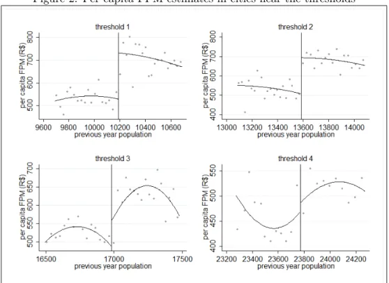
Figure 2 shows the effect of the population rule on FPM per capita received by estimating linear polynomial regressions on the left and right sides of the cutoffs using Calonico, Cattaneo and Titiunik’s (2014b) estimator for RDD graphs. We consider 500 inhabitants windows around the thresholds. The increase in FPM funds per capita based on population rule is strong, especially at thresholds 1 and 2.
Figure 1: Estimates of declared and theoretical per capita FPM for all the sample
4.2 Forcing variable distribution
A number of studies attest to abnormalities in the distribution of municipal population in the regions of the FPM thresholds. Litschig (2012) shows evidence of manipulation since 1991, whereas Monasterio (2013) notes the increase of distortions since 2007. Monasterio (2013) uses the test described in McCrary (2008) for detecting forcing variable distribution discontinuities by estimating local linear regressions, and he finds strong evidence for population manipulation based on the FPM rule.
Additionally, the author uses a method for discriminating among municipalities that change tracks because they are near the thresholds. The author uses a regression to estimate a city’s population in relation to a polynomial of its ranking in the global population distribution. Another specification is then estimated that adds dummies on this regression, indicating whether the municipality is near one of the cutoffs. Analyzing the differences in the two distributions, the author finds 180 municipalities that appear to have manipulated their populations to receive additional transfers. We use 1,000-inhabitant windows to identify the cities near the cutoffs, and we find almost 300 municipalities, in an universe of 4,000, that could be manipulating their populations to be included in higher population bands.
Figure 2: Per capita FPM estimates in cities near the thresholds
Note: Calonico, Cattaneo and Titiunik (2014b) fourth order polynomial estimator. Each dot represents the dependent variable sample average in a given bin.
Figure 5A shows the histogram of the local 2002 population on the left and the 2011 population on the right, using bandwidths of 1000 inhabitants. We take 2002 and 2011 because these are the first and last years that were used to construct the theoretical per capita FPM transferred, remembering that the current year’s FPM depends on the previous year’s estimated population. There appear to be clear discontinuities in 2011, greater than those in 2002. Figure 6B, with the population histogram with a 200-inhabitant bandwidth windows, presents more clear jumps in the 2011 histogram that must be attributable to the FPM distribution rules. Again, this effect is less clear in 2002.
We conclude that the FPM population thresholds causes discontinuities in population distribution. According to Van der Klaauw (2002), Mccray (2008) and Lee and Lemieux (2010), the manipulation and the discontinuity of the forcing variable are not in themselves problems that necessarily bias estimates given that this process is random with respect to variables that could affect the response variables. We should verify if spending responses are potentially the same for cities with very similar populations and that crossing the thresholds is random for cities that are very near them.
Figure 3: FPM population rule impact on budget expenditures
Note: Calonico, Cattaneo and Titiunik (2014b) fourth order polynomial estimator. Each dot represents the dependent variable sample average in a given bin.
close to the thresholds in 2002. There is a concentration of cities shortly after the band changes in 2011, indicating that local municipalities that changed the population brackets maintained a low population growth during the period, as we analyze further in the next subsection.
Figure 6B shows that cities that were far from the thresholds had much less probability of changing population brackets. Cities that did not changed coefficient was in general distant from the thresholds in 2002 population histogram. This may represent a limitation on the possibility of manipulating population, as population can not increase enough to all cities obtain a higher coefficient. Cities seem to enter or leave a given estimation window marginally, probably because population growth is a continuous function of population. For now on, we verify the continuity of population growth estimates, which may ensure the randomness of treatment status near the thresholds.
4.3 Local population growth estimates
Figure 4: FPM population rule impact on neighbor budget expenditures
Note: Calonico, Cattaneo and Titiunik (2014b) fourth order polynomial estimator. Each dot represents the dependent variable sample average in a given bin.
capacity is low and marginal, any type of treatment contamination will not be a problem if it does not alter the mean potential outcomes of the treatment and control groups in vicinities of the thresholds.
We can monitor how cities manipulate their populations analyzing the yearly population growth released by the IBGE. Any influence is not a problem if population growth varies continuously throughout the population, which we would expect if mayors and politicians have only limited influence on this variable. In this case, we expect that municipalities continually enter or leave the regions near the cutoffs and the potential outcomes are still be balanced.
Annual population growth as estimated by the IBGE is based on the methodology developed by Madeira and Sim˜oes (1972). For each administrative unit i’s population, Pi(t), IBGE takes
data on the previous two population counts or the census data from years t= t0 and t1, and also for the population of a higher-level hierarchical unit,P(t), in census years, such that:
P(t) = ΣPi(t)
Figure 5: Histograms of population: 1000 (A), 200 (B) inhabitants windows
Pi(t) = Ω1P(t) + Ω2 (6)
Resolving the system using t = t1, t2 provides Ω1 and Ω2. Thus, for the period between
2002 and 2007, estimates for July of each year are made as follows. First, state populations are updated considering the system withPi(t) as a state’s population in year t and P(t) as Brazil’s
population in years t = 1990,2000. For municipalities smaller than 100,000 inhabitants, as in our sample, municipalities were grouped according to quartiles of cities with similar population growth and population.
Figure 6: Histograms of population: cities that cross (a) and do not cross (b) the thresholds over 2005-2012
was not ready in time to be used for the 2010 and 2011 estimates6 .
Some observations can be noted directly from equation (6). First, the population growth estimates for neighboring municipalities are correlated because both are subject to the same growth shocks in the upper unit. Second, the fact that population growth of superior geographical units, such as country, state or quantile of cities, directly influences local population growth shows that individual cities’ ability to influence own population growth, and, consequently, the FPM population coefficient, is very restricted and limited, as cities can not influence superior units’ growth.
Figure 7A shows that population growth follows an approximately normal distribution, with a mean similar to the national mean, 0.5%. Figure 7B shows the population growth histogram in the period that cities change their population coefficients. We see that their growth is positive and near zero in general, which leads to a buildup of cities just to the right of the thresholds. Local population growth seems to follow a continuous path, even in the periods that cities change population brackets.
Figure 8A presents population growth estimated by local polynomial regression for the
6More information on the methods employed for local population estimation can be found in technical notes,
Figure 7: Histogram of population growth: total (A) and when crossing the thresholds (B)
periods during which municipalities did not change their population brackets. Municipalities that did not change brackets but were near the thresholds had negative or near-zero population growth. The greatest growth cities are, naturally, in the middle of the segments. Cities that have grown more were in general far from the thresholds and did not change population brackets during the period. Municipalities that do not change and are at the beginning of a bracket grow slightly.
Figure 8B presents the polynomial estimations of population growth in cities that had changed population coefficients and in the exact periods that they made the transition. Most municipalities move to a point just after the thresholds, as is clear with the increasing confidence intervals with increasing populations within a bracket. Furthermore, the municipalities do not have negative population growth when changing bands, in the mean, because in nearly all cases, the cities moved to superior population brackets. At the same time, population growth is generally low because there is no way to influence this process, or even because mayors wanted to maintain low population growth in the beginning of brackets to maximize the per capita FPM grant.
Figure 9 shows the estimates of local polynomial regressions of population growth by population size, and there are no clear discontinuities for the municipalities of up to 30,000 inhabitants in the period considered. In this case, nothing indicates that there is an effect of the FPM cutoffs on the growth of cities taken together. An explanation for the population growth continuity at the thresholds is that local populations are estimated from the previous population counts, accounting for both the state and country growth rates (IBGE, 2008).
Figure 8: Polynomial regression of population growth by population size - periods in which municipalities do not cross to a superior bracket (A) and cross to a superior bracket (B)
95% confidence interval
Figure 9: Estimates of population growth
95% confidence interval
to the population rule. We estimate separately local polynomial regressions in windows of 500 inhabitants to the right and to the left of each threshold. The effect of the thresholds on population growth is insignificant for all thresholds, particularly when we compare the effect of population on the FPM per capita, as shown in Figure 2.
Figure 10: Estimates of population growth in cities near the thresholds
Note: Calonico, Cattaneo and Titiunik (2014b) fourth order polynomial estimator. Each dot represents the dependent variable sample average in a given bin.
4.4 Neighbors’ balancing in treatment and control groups
We analyze the balancing of neighbors j due to i’s treatment according to some variables that we expect initially to be exogenous to our experiment, as the number of neighbors and the neighbor’s population. Also, we want to assess the extent of correlation between city i and neighbor j’s FPM. Figure 11 shows the number of neighbors j of cities i that are near the thresholds. This is important because in our regressions we measure the mean effect of neighbors’ FPM on city i’s spending, which is correlated with number of neighbors.
Figure 11: Estimate of number of neighbor in cities near the thresholds
Figure 12 shows that for the first two thresholds, local population is not affected, on average, based on whether neighbors are in treatment or control areas, but cities near thresholds 3 and 4 are even larger when the neighbors are to the right of the cutoffs. These results indicate spillover effects of FPM on neighbor populations, possibly due to local economic development, which leads to the attraction of migrants. This effect in itself implies a fiscal spillover effect due to the per capita reduction in the local revenue and expenditures.
Figure 12: Estimate of neighbor population in cities near the thresholds
Note: Calonico, Cattaneo and Titiunik (2014b) fourth order polynomial estimator. Each dot represents the dependent variable sample average in a given bin.
Figures 13 shows that there is little variation in city i’s FPM grants based on neighbor j’s population bracket variations. We see some correlation between instruments received by i and j, much lower than the impact of the coefficient variation in own spending comparing with Figure 2. The greater effect appears to occur when j is near threshold 3. This correlation must be due to population growth correlation between neighbors, as this is the variable that accounts for the most of FPM variation in the estimation windows. We control for cities i and j’s populations, as the per capita FPM received by both cities, in order to avoid the bias caused by spillover of FPM grants.
5
Results
5.1 FPM impacts in all cities with fewer than 30,000 inhabitants
Figure 13: Estimate of neighbor FPM in cities near the thresholds
Note: Calonico, Cattaneo and Titiunik (2014b) fourth order polynomial estimator. Each dot represents the dependent variable sample average in a given bin.
Ordinary Least Squares (OLS), Fixed Effects (FE), and Instrumental Variables with Fixed Effects (FE-IV), the latter considering theoretical FPM as an instrument in the first stage. These results are shown in Table 1, which is separated by three specifications for different independent variables and displaced from the top to the bottom: (1) using only F P Mi, (2)
using onlyF P Mj and (3) using bothF P Mi and F P Mj.
Specification (1) of Table 1 considers the effect of city i’s FPM on i’s spending, and shows that the FPM generates a more than proportional impact on the municipality’s total expenditures, which is called the crowding-in effect in the literature. Spending on education, health, urban planning and sanitation is positive and statistically impacted, with greater effects on education and health spending. We also observed that OLS effects are the smallest and that EF estimates are greater than FE-IV estimates, with the exception of the sanitation spending function.
Specification (2) of Table 1 shows the results of neighbor j’s FPM spillover on city i’s expenditures, and these are considerably lower than the own FPM impacts that were presented in specification (1). An exogenous R$1 increase in FPM received by j increases total spending by 50 cents using OLS regressions and approximately $1.62 using FE-IV. Spending on health and education, municipalities’ major expenditure categories, increases by 13 and 11 cents, respectively, using OLS regressions. Considering the FE-IV estimation, the impacts are 45 and 42 cents, respectively. All results are significant at the 1% level.
We present in specification (3) of Table 1 the results of regressions in which we use both
F P Mi and F P Mj as independent variables at the same time. Both variables are significant
variables separately. Specially, spillover estimates are much lower than before. The effect on spending using FE is 10 cents lower, whereas the FE-IV estimates were 45 cents lower, less than one-third of the estimates from part (2).
Estimates of the impact of i’s FPM on its own expenditures are much closer to the coefficients that were estimated in specification (1). This shows that the correlation between a municipality’s own FPM grant and its spending is very high, whereas the additional explanation of the variable
F P Mj is very low, which is clear from the observation of R2 of OLS regressions. F P Mj alone
appears to explain 4 % of i’s expenditures, but adding F P Mj to specification (1) does not
increase regressionR2.
[Table 1]
5.2 Impacts of FPM using the discontinuity rule
Next, we estimate the effect ofF P Mi andF P Mjon city i’s expenditures using RDD regressions,
considering that i and j have populations within 500 inhabitants of the thresholds. We consider for all of the following regressions in this subsection that cities i and neighbors j are in windows around different thresholds, even in the regressions that control for only one FPM. We use 2SLS in Fixed Effects (FE-IV), including theoretical FPM as instruments for i and j’s declared FPM grants.
Table 2 shows the effects of F P Mi and F P Mj, estimated separately and together, on city
i’s budget expenditures. The first 4 columns show the results for the variables by level, and the last 4 columns present elasticities estimated by regressions with the variables transformed into logarithms, with the exception of population and its quadratic term. In each column, we control for population i in one of the four discontinuity windows at the top or for population j at the bottom. Controlling only for F P Mi, the effect of R$1 extra FPM on spending is significantly
particular, the effect at threshold 1 decreases from 0.88% to 0.57%. At the same time, the spillover effect ofF P Mj is only significant and positive when city i is at threshold 1, and so j’s
population is greater than i’s.
We present at the bottom of Table 2 spillover estimates in which we control for neighbors j near each of the thresholds. The coefficient ofF P Mj, the spillover effect of the grant, without
controlling for F P Mi, is in general similar to the estimated effect of F P Mi alone in the first
part of the table, maybe due to the correlation of FPM between cities i and j. These effects are R$1.66 when neighbor j is near the first thresholds, R$2.75 and R$2.28 at thresholds 2 and 3, and R$3.19 when neighbor j is at the last threshold. Controlling forF P Mi reduces the
F P Mj spillover effect, which is no longer significant at 10% at thresholds 1 and 4. Additionally,
theF P Mi impacts are lower when city i is not at these thresholds. F P Mj elasticity, without
controlling for logF P Mj, on expenditures per capita is 0.79% at the first threshold, whereas at
the other thresholds, the values are statistically very close to 1%. There is again a reduction in the magnitude and significance ofF P Mj effects with the addition of the logF P Mi. The spillover
effect remains only in the intermediate tracks, and bothF P MiandF P Mj are insignificant when
j is at threshold 4.
[Table 2]
In Table 3, we repeat the procedures from the previous table, replacing budget spending with health spending as the dependent variable. The effects of a municipality’s own FPM grant, without controlling for F P Mj, are positive and significant. The impacts estimated with level
variables show an increasing effect from the first to the third population thresholds, ranging from R$0.55 to R$0.78. The effects estimated with level variables and withF P Mj as the control are
lower, especially at threshold 1, and are insignificant for the municipalities at threshold 4. The effects continue to increase with population increases up to the third threshold, ranging from R$0.29 to R$1.02.
The effects with log variables without controlling forF P Mj are generally close to 1% except
for the third threshold, where the estimated impact is 2.16%. By controlling for F P Mj, the
effect of 2.28% on health spending when i is at threshold (3), that is, municipalities would spend more on health if there were no FPM spillover effect received by neighbors j. In this case, j usually has a lower population than i, according to population distribution in Section 4, which shows that city i spends less on health when their neighbors are smaller and receive larger FPM grants.
Table 3 also presents estimates of j’s FPM spillover effects on city i’s health spending, controlling for the neighbor j’s threshold, first without controlling for the FPM received by i. The estimates are small, ranging from R$0.45 to R$0.81 for level regressions, values statistically lower than R$1. Adding F P Mi, the spillover effect is R$0.53 at threshold 3, whereas becomes
insignificant at the others. The impact of F P Mi is significant only when j is near the first or
second thresholds, when i’s population is usually larger than j’s. Regressions with log variables show that the spillover effect on health spending, without controlling forF P Mi, is statistically
equal to 1%, except at the first threshold, where the effect is 0.7%. Controlling for F P Mi,
the elasticities of F P Mj when j is near the first or second population thresholds are -0.72%
and -2.59%, respectively, and elasticity is positive on the third threshold, 0.75%. These results, significant at 1%, confirm that the estimated j’s FPM spillover effect on i’s health spending is negative when neighbor j is smaller than i, and positive otherwise. In this situation, neighbor j’s population benefits more from city i’s spending on health than the opposite, so an increase in neighbor j’s health spending may decrease total demand for health services in city i.
[Table 3]
The impacts of FPM grants on education spending are shown in Table 4. The first part shows that the impact of a municipality’s own FPM grant, without controlling for neighbors’ grants, increases with the municipality’s own population from R$0.53 to R$0.98 for each R$1 per capita transferred from thresholds 1 to 4. The level effects range from R$0.37 to R$0.83 between the first and third thresholds when we add F P Mj, and spillover effects are not significant at
5%.
The results using log variables are statistically close to 1%, except at the first threshold, 0.76%. Again, the impacts increase with population and reach 1.23% at threshold 4. The elasticities ofF P Mi when we add the logF P Mj do not change statistically at thresholds 2 and
The spillover effect is 0.43% when city i is on the first threshold and j is bigger, value significant at 5%.
The lower part shows the regression results in which we control population j in each of four RDD estimation windows. The level spillover effect, without controlling for i’s FPM, is R$0.57 for the smallest population group and R$1.02 for the largest group. The spillover effects, when we add city i’s FPM, remain significant only at the second and third thresholds, R$0.61 and R$0.46. The spillover elasticities, without controlling for F P Mi, on education spending are
statistically close to 1%. When we add the log of city i’s FPM grant, the estimates become insignificant at the 5% confidence level.
[Table 4]
The estimated effects of FPM on urbanization spending are in Table 5. The effects by level are lower than those estimated for education and health spending and very lower than R$1, but are still significant at 1%, ranging from R$0.15 to R$0.56 when we do not control for neighbors’ FPM . The effects of a municipality’s own FPM are reduced when we include neighbors’ FPM grants and are insignificant on the second and fourth tracks. The effects are only significant at 1% for municipalities at threshold 3, a increase of R$0.35.
The F P Mi elasticity in urban spending, without controlling for F P Mj, is greater than 1%
for municipalities on the third and fourth RDD windows, with values of 1.74% and 1.88%, and close to 1% when i is in the first or second estimation windows. By adding the log ofF P Mj, the
elasticity ofF P Mi is 2.62% at threshold 3, significant at 1%, 1.42% at threshold 1, significant
at 5%, while insignificant at 10% at the other thresholds. The effect of the log F P Mj is only
significant at 10% when i is at threshold 3, -1.26%.
The bottom part of Table 5 shows the results after controlling for population j in each of the four RDD estimation windows. The results are generally positive and significant at 1% when we do not control for F P Mi, ranging from R$0.23 to R$0.42. By adding F P Mi, most of the
estimated effects of F P Mj lose significance at 5%, except when neighbors j are in estimation
window 3, R$0.22.
The estimated elasticities follows the same trend of regressions using level variables. The effects ofF P Mj without controlling forF P Mi are positive and statistically close to 1%, except
the thresholds, whereas the effect of F P Mi is significant at 5% when j is in the first or second
windows, increasing urban spending by 1.67% and 1.85% respectively.
[Table 5]
Finally, Table 6 shows the results for spending on basic sanitation - the function of budget spending with the lowest amount applied in our sample. The estimated effects for a municipality’s own FPM, using level variables and without considering neighbors’ FPM grants, are insignificant at 5% at thresholds 1 and 2 and significant at this value at thresholds 3 and 4, although the effects are very small, R$0.08 and R$0.07 respectively. The level effect ofF P Mi when we control
for F P Mj only remains significant at 5% when i is at threshold 3, R$0.23, as well as F P Mj
spillover impact, -R$0.15 in this case.
The effect of log F P Mi without controlling for log F P Mj is only significant at 5% at
threshold 3, 4.38%, which increases to 16.12% when we control forF P Mj. At the same time,
there is a strong negative spillover at this threshold of -9.59%. The elasticities of F P Mi and
F P Mj are insignificant at 1% in the other groups.
The effect of neighbor j’s FPM grants, without controlling for city i’s FPM grant, on sanitation spending are only significant at threshold 3, R$0.12 for the level regression and 6.91% for log estimates. Spillover effects on sanitation are more significant when we include i’s FPM. The effect level is significant at 5% when j is close to threshold 1, - R$0.12, and in the log estimation, -5.96%. At the same time, the values are positive and significant at 5% for municipalities at threshold 3, R$0.21 for level variables and 13.79% for log variables.
These results show a substitution effect between neighbors’ FPM grants and spending on sanitation, as happens with health expenditures. Basic sanitation is very deficient in Brazilian small cities, which is one of the most important causes of diseases and demanding public health system. the spillover effect ofF P Mj is greater when j is in the first estimation window, that is,
when j is smaller than i. Increasing sanitation spending in neighbor j, when j is smaller than i, may decrease demand for i’s health services and even decrease i’s health spending. Moreover, the decrease on health demand may lead to city i’s mayor invest less in sanitation.
6
Alternative sample of neighbors
The developed analysis shows that thinking about a municipality’s own FPM per capita as a quasi-experiment to measure the impacts of transference on expenditures may be misleading if we do not consider neighbors’ conditions, due to correlations between neighbors’ FPM grants. In experiment design literature, we should say that increasing i’s probability of being treated increases the probability of j’s being treated, so not controlling for both cities’s treatment status may lead to bias in the estimates.
Another way to avoid FPM interactions between municipalities and their neighbors is to select an appropriate sample of neighbors j that lie outside of any of the RDD windows, in which case the probability of both cities i and j changing population coefficient simultaneously is considerably reduced7. In this case, small population growth may change the treatment status of i but not that of j, so we can identify a given municipality’s own FPM impacts. Conversely, we can measure spillover effects controlling for neighbors j in one of the RDD window and cities i out of them.
Table 7 showsF P Mi impacts on i’s spending by function. We perform 2SLS-FE regressions
using level variables and considering the FPM grant received by municipality i at each of the thresholds; initially, we consider all of the thresholds together. On the left side of the table, we consider regressions without controlling forF P Mj. Overall, the estimates are relatively close to
those that were previously calculated. On the right side of the table, we repeat the regressions with the addition of F P Mj. We consider the aggregate FPM grant received by neighbor j in
place of the per capita values because population can be influenced by spillover effects.
The changes are much smaller than those found in Tables 2–6 . Estimated variances increase when we control for j’s FPM, but they are much smaller than those that are exposed in Tables 2–6, indicating a bigger sample and weaker correlations between the cities i and j’s FPM. The total budget spending shows the greater difference in the estimated values with the inclusion of
F P Mj, although this difference is not statistically significant except when we consider all the
thresholds together.
[Table 7]
The estimates for neighbor j’s FPM spillover effect, with j in the RDD windows, on city i,
outside of the windows, are shown in Table 8. The results of 2SLS regressions without adding the aggregate FPM grants received by i as controls are on the left side. The estimates are larger than those that we found previously. In this case, as is clear by the histogram in Figure 5, most cities i have fewer than 10,000 inhabitants and so are smaller than i, showing again that the spillover effect of neighbor j on city i is greater when j is larger than i.
The right side repeats the estimation spillover with the addition of the FPM grant received by i as the control. Spillover effects on overall expenditures decrease with the addition of municipality i’s FPM grant. Estimates are significant in all specifications. The effects estimated for the FPM amounts that were added as controls are null to two decimal places, for all regressions performed in this Section, which is further evidence of the validity of the instrument in this sample.
[Table 8]
Finally, we estimate the spillover effect on city i’s population when j is within the RDD windows and i is not. The upper part of table 9 shows the results for level variables. The estimated effects without controlling for i’s FPM are significant for all thresholds and increase with j’s population, and there is an increase of one person for each R$1 per capitaF P Mj when
j is close to threshold 4. The right side shows that the level spillover effect when controlling forF P Mi becomes statistically null for all thresholds considered together and for the first and
second thresholds, whereas the effects are positive for thresholds 3 and 4. The estimated effects with the variables in logs show an elasticity between the thresholds that varies from 0.03% to 0.06%, except for cities j that are at the first threshold, 0.01%, and the results are similar when we control for i’s FPM. Spillover effects of neighbor j’s FPM on city i’s population may be one cause of the FPM correlations between neighbors.
These results indicate that population mobility is an important variable for fiscal interaction in Brazilian cities, as population is the only variable that can increase local FPM over the short term. Moreover, correlation among populations may be due to FPM itself. One possibility is that cities compete with each other attracting population for receiving extra grants. Also, local development due to the extra grant may lead to migration from other regions.
7
Extra robustness checks
We conduct additional tests to assess the robustness of our results to different specifications. Table 10 of Appendix A presents RDD estimations excluding the years in which there are population discontinuities, based on the McCrary (2008) tests in Figures 14 and 15. We take logarithms of the variables, with the exception of population, and we exclude the years 2008, 2011 and 2012, remembering that a given year’s population is used to estimate the following year’s FPM. The left-hand table shows the results without controlling for neighbor j’s FPM and an elasticity on expenditures usually slightly above the previously calculated - especially for cities near the first threshold.
Controlling for F P Mj on the right side, a municipality’s own FPM effects are typically
reduced, and neighbor spillover is insignificant in nearly all cases; the exception is FPM spillover on health spending at threshold 3, for which there is a reduction of 2.4% for each 1% increase in neighbor FPM. Two factors explain the general loss of significance: first, a reduction of nearly one-third of the sample size, and second, the reduction on treatment status variation, which reduces the sensitivity of the fixed-effects estimator. Discontinuities in population distribution are attributable to the population count in 2007 and the population census in 2010. In this years, the parameters that are used to estimate population growth in the inter census years changed. The exclusion of these years implies excluding most of the exogenous FPM variation that is not correlated through time and between cities i and j.
We present in Table 13 of Appendix C the results when we control for neighbor j’s spending, considering the variables in logarithms, in which that we do (the right side) or do not (the left side) control for neighbor j’s FPM. The effects of a municipality’s own FPM are generally statistically smaller than those that were previously estimated in both specifications. The effect is nearly always less than 1% for each 1% additional FPM per capita received. This result indicates that budget expenditure spillover accounts for part of a municipality’s own FPM impacts. Spillover effects of neighbor j’s FPM grants on city i’s expenditures decrease, as observed on the right side of the table, which is explained by the high correlation between FPM and per capita spending. F P Mj spillover effects on health and sanitation spending are still
negative and significant at 1% when city i is close to the third threshold.
8
Conclusions
To what extent the impacts of an unconditional grant to a municipality i will be affected if i’s neighbor also receives the transfer? We estimate the effects of a federal grant, the Municipalities’s Paticipation Fund, the FPM, on municipal expenditures, also considering the spillover impacts of the neighbor’s grant. We use a rule of transfer that is based on population brackets, which creates discontinuities at the 4 thresholds considered for the Regression Discontinuity Design (RDD). Thus, we can estimate the extent to which the response to FPM grant that is received by city i in window ni is related to j’s FPM grant in window nj, with ni 6= nj. In these
municipalities, receiving the FPM grant should be correlated given that the probability of treatment is influenced by population growth, which is correlated among neighbor cities. We estimate own and spillover effects separately by controlling for i and j’s FPM in the same time. Effects of i’s FPM on i’s spending are in general positive and significant, but the values are reduced when we control for F P Mj, as there is a positive spillover in most of the cases. The
effects on municipalities that are close to threshold 4 are not significant when we control for j’s FPM, indicating a high correlation between cities i and j’s treatment status, possible due to population correlation. Elasticity of j’s FPM on i’s education and urbanism spending are positive, indicating a complementary of these expenditures between neighbors i and j, but the elasticities ofF P Mj on city i’s health and sanitation expenditures are negative when j is smaller
the demand of city j’s population for city i’s public health provision may decrease, and city i’s spending on health may decrease as well.
We perform alternative estimations of FPM spillover impacts using neighboring municipalities that are outside of the RDD windows. The estimates for this sample are less affected by the inclusion of neighbors’ FPM, and they generally retain their significance, because in this case the city has much more chance of being treated than its neighbor. These results indicate that the estimates of the FPM impacts may change due to the chosen sample of neighbors. Finally, we estimate the spillover effect on neighbor population, which is positive and significant, specially at thresholds 3 and 4. FPM spillover effects on population mobility may explain part of the population correlation and fiscal interaction among Brazilian municipalities.
References
[1] Acemoglu, D. and Angrist, J. (2000). How large are human-capital externalities? Evidence from compulsory-schooling laws.NBER Chapters, NBER Macroeconomics Annual, National Bureau of Economic Research, 15, 9-74. [2] Angelucci, M. and De Giorgi, G. (2009). Indirect effects of an aid program: how
do cash transfers affect ineligibles’ consumption? American Economic Review, 99(1), 486–508.
[3] Angelucci, M. and Di Maro, V. (2010). Program evaluation and spillover effects.
Impact-Evaluation Guidelines, Technical Notes, Inter-American Development Bank, No. IDB-TN-136.
[4] Angrist, J., Imbens, G. and Rubin, D. (1996). Identification of causal effects using instrumental variables. Journal of the American Statistical Association, 91(434), 444–472.
[5] Angrist, J. and Lavy, V. (1999). Using Maimonides’ Rule to estimate the effect of class size on scholastic achievement.The Quarterly Journal of Economics, 114(2), 533-575.
[6] Arvate, P. , Mattos, E. and Rocha, F. (2013). Conditional versus unconditional grants and local public spending in Brazilian municipalities. 35th Meeting of the Brazilian Econometric Society, Foz do Iguacu, Brazil, December.
[7] Besley, T. and Case, A. (1995). American Economic Review, 85, 25-45.
[8] Bordignon, M., Cerniglia, F. and Revelli, F. (2003). In search of yardstick competition: a spatial analysis of Italian municipality property tax setting.
Journal of Urban Economics, 54(2), 199-217.
[9] Brollo, F., Nannicini, T., Perotti, R. and Tabellini,G. (2013). The Political Resource Curse.American Economic Review, 103(5), 1759-1796.
[11] Brueckner, J. and Saavedra, L. (2001). Do local overnments engage in strategic property-tax competition? National Tax Journal, 54(2), 203-230.
[12] Buettner, T. (2003). Tax base effects and fiscal externalities of local capital taxation: evidence from a panel of German jurisdictions. Journal of Urban Economics, 54(1), 110-128.
[13] Calonico, S., Cattaneo, M. and Titiunik, R. (2014a). Robust nonparametric confidence intervals for Regression-Discontinuity Designs. Econometrica, 82(6), 2295–2326.
[14] Calonico, S., Cattaneo, M. and Titiunik, R. (2014b). Robust data-driven inference in the Regression-Discontinuity Design.Stata Journal, 14(4), 909-946.
[15] Case, A., Rosen, H. and Hines, J. (1993). Budget spillovers and fiscal policy interdependence: evidence from the states.Journal of Public Economics, 52(3), 285-307.
[16] Castro, M. and Regatieri, R. (2014). Impacto do Fundo de Participac˜ao dos Munic´ıpios sobre os gastos p´ublicos por func˜ao e subfun¸c˜ao: an´alise atrav´es de uma regress˜ao em descontinuidade. 42 Encontro Nacional de Economia, Natal, Brasil, December.
[17] Devereux, M., Lockwood, B., Redoano, M. (2007). Horizontal and vertical indirect tax competition: Theory and some evidence from the USA. Journal of Public Economics, 91(3-4), 451-479.
[18] Devereux, M., Lockwood, B., Redoano, M. (2008). Do countries compete over corporate tax rates? Journal of Public Economics, 92(5-6), 1210-1235.
[19] Figlio, D., Kolpin, V. and Reid,W. (1999). Do states play welfare games? Journal of Urban economics, 46(3), 437-454.
[20] Gadenne, L. (2011). Tax Me, But Spend Wisely: The Political Economy of Taxes, Theory and Evidence from Brazilian Local Governments.Northeast Universities Development Consortium Conference 2011, Yale University, New Haven, USA. [21] IBGE - Instituto Brasileiro de Geografia e Estat´ıstica (2004). Proje¸c˜ao da
popula¸c˜ao do Brasil por sexo e idade – 1980-2050: Revis˜ao 2004. Rio de Janeiro, RJ: IBGE.
[22] IBGE - Instituto Brasileiro de Geografia e Estat´ıstica (2008). Proje¸c˜ao da popula¸c˜ao do Brasil por sexo e idade – 1980-2050: Revis˜ao 2008. Rio de Janeiro, RJ: IBGE.
[23] Imbens, G. and Lemieux, T. (2008). Regression Discontinuity Designs: A Guide to Practice.Journal of Econometrics, 142, 615–635.
[24] Imbens, G. and Wooldridge, J. (2009). Recent developments in the econometrics of Program Evaluation.Journal of Economic Literature, 47(1), 5-86.
[25] Isen, A. (2014). Do local government fiscal spillovers exist? Evidence from counties, municipalities, and school districts. Journal of Public Economics, 110(C), 57-73.
[27] Knight, B. and Schiff, N. (2010). Spatial competition and cross-border shopping: Evidence from State Lotteries [Working Paper No 15713]. National Bureau of
Economic Research, Cambridge, MA.
[28] Lee, D. and Lemieux, T. (2010). Regression Discontinuity Designs in Economics.
Journal of Economic Literature, 48(2), 281-355.
[29] Litschig, S. (2012). Are rules-based government programs shielded from special-interest politics? Evidence from revenue-sharing transfers in Brazil.
Journal of Public Economics, 96(11-12), 1047-1060.
[30] Litschig, S. and Morrison, K. (2012). Government spending and re-election: Quasi-Experimental evidence from Brazilian municipalities [Working Paper No 515].Barcelona Graduate School of Economics, Barcelona, BA.
[31] Litschig, S. and Morrison, K. (2013). The impact of intergovernmental transfers on education outcomes and poverty reduction.American Economic Journal: Applied Economics, 5(4), 206-240.
[32] Madeira, J. L.and Sim˜oes, C. (1972). Estimativas preliminares da popula¸c˜ao urbana e rural segundo as Unidades da Federa¸c˜ao, de 1960/1980 por uma nova metodologia. Revista Brasileira de Estat´ıstica, 33(129), 3-11.
[33] Mccrary, J. (2008). Manipulation of the running variable in the regression discontinuity design: a density test.Journal of Econometrics, 142(2), 698-714. [34] Mendes, C. and Sousa, M. (2006). Demand for locally provided public services
within the median voter’s framework: the case of the Brazilian municipalities.
Applied Economics, 38(3), 239-251.
[35] Miguel, E. and Kremer, M. (2004). Worms: identifying impacts on education and health in the presence of treatment externalities.Econometrica, 72(1), 159–217. [36] Minist´erio da Fazenda (2005). O que vocˆe precisa saber sobre transferˆencias
constitucionais.Bras´ılia: Minist´erio da Fazenda, Secretaria do Tesouro Nacional. [37] Minist´erio da Fazenda (2012a). O que vocˆe precisa saber sobre transferˆencias constitucionais e legais: Fundo de Participa¸c˜ao dos Munic´ıpios - FPM. Bras´ılia: Minist´erio da Fazenda, Secretaria do Tesouro Nacional.
[38] Minist´erio da Fazenda (2012b). Manual de contabilidade aplicada ao setor p´ublico: aplicado `a Uni˜ao, aos Estados, ao Distrito Federal e aos Munic´ıpios - procedimentos cont´abeis or¸cament´arios. Bras´ılia: Minist´erio da Fazenda, Secretaria do Tesouro Nacional.
[39] Monast´erio, L. (2013). O FPM e a estranha distribui¸c˜ao da popula¸c˜ao dos pequenos munic´ıpios brasileiros. [Texto para discuss˜ao No. 1818]. Bras´ılia, DF: IPEA.
[40] Nickerson, D. W. (2008). Is voting contagious? Evidence from two field experiments.American Political Science Review, 102(1), 49–57.
[41] Persson, T. and Tabellini, G. (1996). Federal Fiscal Constitutions: Risk sharing and moral hazard.Econometrica, 64(3), 623–646.