Project Subcontractors Selection in Fixed Price and Cost-plus Contracts



Abstract _{— Depending on your view of the allocation of}

risk between the project owner and contractor use are two main types of contracts. In this paper, we analyze the problem of optimal selection of sub-contractors in the case of the application of a fixed price and a cost-plus contracts. Models described in the article can be found applicable in the relations between the project owner and the contractor and between the contractor and sub-contractors.

As a methodological basis we use the multi-criterial decision model assigning each task to specific contractors (or sub-contractors) in the project with the function of distribution of penalties arising from delayed completion and potential benefits in the event of early termination of the project.

Index Terms— project procurement, subcontractors selection, fixed price contracts, cost-plus contracts

I. INTRODUCTION

he issue of contract management and procurement management is one of the fundamental problems in the practice of project management. Its importance is highlighted in the one of the most common project management methodologies - PMBoK [8] of the Project Management Institute, which gives it one of the nine areas of knowledge. As the process of " Plan contracting" indicates selection of a sub-contractors cannot be planned without taking into account the relationship between the "project schedule”, "activity cost estimations", " activity resource requirements", and “Project Management Plan” with its components focused on “risk register” and “risk-related contractual agreements”. Therefore, we believe that the process of selecting a contractor must include the methodology used to create the schedule in accordance to the policy of distribution of risks between the project owner and the contractor.

Classical scheduling methods of CPM (Critical Path Method) and PERT (Program Evaluation and Review Technique) do not explicitly take into account the factors associated with the uncertainty that surrounds the choice of the contractor and his participation in the implementation of the project scope. Therefore, in the later part of the paper we

Manuscript received July 19, 2013; revised July 12, 2013. The project was funded by the Polish National Science Centre on the basis of the decision number DEC-2011/03/D/HS4/01649.

P. Blaszczyk is with the University of Silesia, Institute of Mathematics, Bankowa 14, 40-007 Katowice, Poland (phone: +48-32-258-29-76; fax: +48-32-258-29-76;; e-mail: pawel.blaszczyk@us.edu.pl).

T. Blaszczyk is with Department of Operation Research, University of Economics, 1 Maja 50, 40-287 Katowice, Poland (phone, fax: +48-32-257-74-71; e-mail: tomasz.blaszczyk@ue.katowice.pl).

use assumptions described by Błaszczyk et al. [3] in terms of the bi-criterial model of project with time and cost buffers designed based on the concept of CCPM (Critical Chain Project Management).

Concept of Critical Chain (Goldratt [4]) is one of the Newest project management methodologies. However, it is not impeccable (compare Herroelen and Leus [6], Rogalska

et al. [9] Van de Vonder et al. [11]), is a balanced

combination of CPM with the recognition of the overall uncertainty and the impact of the human factor in the planning and implementation of projects. Many later results (for example as described in review by Van de Vonder et al.

[12], [13]) is based on the concepts set forth in the buffers. In some industries (mainly IT) in later years has also found widespread the class of agile [1] methods like XP - eXtreme Programming, Scrum, Lean Software Development. These methods assume the collaboration between client and the contractor including, among others the dynamic adjustment of the schedule and budget for the project to imprecisely specified range, which can also evolve as the work progresses. This approach can be effective, but we must keep in mind that in many business environments, it is not acceptable because of the uncertainty of the final price of the contract for construction of the project. Therefore, we would not consider them later in this paper. Instead, we will focus on the method resulting the concept of CCPM. We will also present considerations for the two types of contract, without indicating which one is more appropriate for a particular project owner. The choice of the type of contract should be determined for a detailed analysis of the type of project, its associated risks and project owner’s risk management policies.

The chain and time buffers quantification methods were the results of successive authors. One of the detailed approaches was formally described by Tukel et al. [10]. The issues of buffering some project characteristics, other than duration, were considered by Leach [7], Gonzalez et al. [5], Błaszczyk and Nowak [2]. The model featured in the next part of this research takes into account the use of partition function the bonus fund for early implementation of the project.

The problem of cost and time overestimation occurs in the present case twice: firstly between the client and the general contractor of the project (related by the contract with the client) and after that between the subcontractors (performing partial ranges of the project) and a general contractor. Hence, if we assume that overestimations of cost and time act consistently in contracting relationships between client and contractor, and between contractor and sub-contractor, than estimations of cost and/or the schedule

Project Subcontractors Selection in Fixed Price

and Cost-plus Contracts

Paweł Błaszczyk, Tomasz Błaszczyk

given to the project owner will be based on data twice overestimated. On the other hand, there are also lots of cases of under-estimations that are evaluated by the project owner in order to select contractors. The reason for this phenomenon is to seek bidders to obtain the best evaluation in the selection phase at the expense of an increased risk of non-compliance with contractual provisions. In order to increase project owner’s safety in similar to the consequences of actions that may result in extending the time for implementation the mechanism of contractual penalties applies. Such a mechanism causing that the bi-criterial time-cost trade-off can be represented as a single-criterial problem and can be applied in both considered contract types. Any exceeding the agreed deadline for completion of the project or any part of it results in measurable, and the financial consequences set before. When this decision problem is analyzed by the general contractor, it is necessary to take into account both the cost of penalties that the general contractor will be forced to pay for the customer, as well as any income from fines paid by its subcontractors. Also the type of the contract has influence how to select the subcontractors. Therefore, it appears appropriate to use for the design of the model of sub-contractors selection both the information about contract type and the concept of time and the cost of buffers. In this case such models can be used as a tool to compensate for liabilities and cash flows.

II. METHODOLOGY

We consider a project which consist x₁,,x_n tasks characterized by cost and time criteria. As the consequence of the contract between the project owner and the contractor there are contracted budget K_max and contracted duration

max

T of the project. Moreover there are defined priceIp, success fee Sp and penalty fee Pp. For example the success fee and the contract penalty fee can be defined as follow:

/ /

p s p

p p p

S r I day

P r I day

 

  (1)

where r_s and r_p are success rate and penalty rate respectively. We assume that we have q potential subcontractorsfor n tasks in the project. Let us consider the following matrix X:

11 1

1

q

n nq

x x

X

x x

 

 

  

 

 



  



(2)

Elements of the matrix Xequal 0 or 1. If x_ij equals 1 it means that subcontractor j submit a bid for task x_i. In the other case there is no such bid for taskxi. The matrix X we will call the subcontractor’s matrix.

A. The fixed price contract

In our first model we assume that between project owner and the contractor there is contract with the fixed price. Let

1, , ; 1, , ij _{i n j q}

K   k _{ }

  (3)

to be the matrix of cost’s of all subcontractors for all tasks and let

1, , ; 1, , ij _{i n j q}

T    t _{ }

  (4)

be the matrix of amounts of work for each subcontractors in each task. Denote by ki the cost of the task

x

i and by ti duration of the activity xi. Thus the total cost and the total duration of the project are given by

1 n

c i

i

K k







(5)

and





1, , max

c i i

i n

T ES t



 

 (6)

where ESi is the earliest start of task

x

i. Contracts with all

subcontractors can also include success fee s_i and penalty fee pi. Also let

1, , ; 1, , ij _{i n j q}

A   a _{ }

  (7)

to be the subcontractors assign matrix. Elements of the matrix

A

equal 0 or 1. If aij equals 1 it means that subcontractor j will be perform task

x

_i. Moreover, let

1, , ; 1, ,n ij _{i n j}

M   m _{ }

  (8)

denote the preference matrix. Elements of the matrix

M equal 0 or 1. If m_ij equals 1 it means that the task i

should be realized together with task j by the same subcontractors. Of course there are ones on the main diagonal. On the other hand let matrix

1, , ; 1, ,n ij _{i n j}

D   d _{ }

  (9)

denote the restriction for tasks in project. Elements of the matrix Dequal 0 or 1. If d_ij equals 1 it means that the task i

could not be realized together with task j by the same subcontractors. In our case we have the following optimization problem. In order to simplified the calculation let us also introduce the following vectors

and

dDI (11)

where

1, , ; 1, ,n ij _{i n j}

I i

 

 

     is an identity matrix. Under the

following assumptions we maximize the total benefits of the project. In our case we have the following optimization problem





      1 1,..., 1 1,..., 1 max 1,..., max 1 1 1,...,q 1 1 1,...,q 1 1 max 0,1 1 1 max 0, 0 n

p p p ij ij ij ij ij

i

ij n

i n ij

j n

i n ij ij

j

c _{i n} i i

q n

c ij ij

i j

n n

j ij ij ik i

i k

n n

j ij ij ik

i k

I S P a x k s p

a

a

a x

T ES t T

K a k K

a x m m

a x d

                                 













 ,di

(12)

where ES_i is the earliest start of task

x

_i, TC denotes total duration of the project, and K_Cdenotes the total cost of the project T_max, Kmax denotes maximum duration and cost for the project respectively. The Tmax, Kmax are results of the project requirements. It leads to find the optimal work assignments for every factor in each activity. From the set of alternate optimal solutions we choose this one, for which the total duration of project is minimal.

B. The cost-plus contract

In our second model we assume that the project will be settled by the cost-plus formula on the basis of the quantity survey.

Like in previous model let cost and duration matrices be given by formulas (3) and (4) respectively. In this model we treat cost from matrix (4) as the cost of actual implementation of each task for each subcontractors. Moreover let

1, , j _{j n}

G   g _

 (13)

be the vector of profit margins for all subcontractors. The values g_j belongs to the interval

 

0,1 . To protect against the uncontrolled growth of the cost of the task

x

_i in such type of contracts the so-called ceiling price is used. So let

 

i i1, ,n

C c _ (13)

Be the vector of ceiling price for each tasks. Like in previous case denote by k_i the cost of the task

x

_i and by t_i

duration of the activity xi. Thus the total cost of the project is given by

1 n

c i i

i

K k g







(14)

where g_i is the profit margin of that subcontractor who will perform the task x_i. The total duration of project is given by formula (6). Like in previous model let subcontractor assign matrix, preference matrix and restriction matrix be given by formulas (7)-(11) respectively. Under the following assumptions we maximize the total benefits of the project. In our case we have the following optimization problem









      1 1,..., 1 1,..., 1 max 1,..., max 1 1 1,...,q 1 1 1,...,q 1 1 1 max 0,1 1 1 max 0, n

p p p ij ij ij j ij ij

i

ij n

i n ij

j n

i n ij ij

j

c _{i n} i i

q n

c ij ij

i j

n n

j ij ij ik i

i k

n

j ij ij ik

i k

I S P a x k g s p

a

a

a x

T ES t T

K a k K

a x m m

a x d

                                 













 





1,..., 1 0, 1 n i n

i n ij ij ij j i

j

d

a x k g c

     





(15)

III. EXAMPLE

Let us consider the simplified example of typical software development project. In the following project we want to design and implement a software with three functionalities. The whole project was divided into 22 tasks A A₁, , ₂ ..., A₂₂. At the beginning we should define the problem (task A₁), describe the requirements (task A2) and action plan (task

3

A ). After that each functionality should be designed (tasks A4, A5, A6). Also some functionality integration should be

done. After the phase of designing the functionality each of them should be implemented (tasks A8, A9, A10) and tested

(tasks A11, A12, A13). Also all of the functionalities should be

tested together (task A17). Next necessary improvements in each functionality should be done (tasks A14, A15, A16). After

that all of the functionalities should be integrated together. After that the whole program should be implemented into our customer environment (task A19). After that some improvements may be necessary (task A₂₀). At the end the customers employees should be learned how to use this program (task A21) and some marketing should be done (task A₂₂).

Project Gantt chart network is represented on Figure 1. These tasks can be performed by subcontractors or by ourselves. In the first step of the procedure we collect bids from subcontractors and note their estimation of the time and costs required to complete this project. In this way we can construct the matrix of subcontractors X, time and cost matrices T and K respectively. Consider the first of the models. Let us assume that in our case we received bids from three potential subcontractors. Moreover part of the tasks we want to perform ourselves. The values of elements in matrix X are given in Table I:

TABLE I

THE SUBCONTRACTORS INFLUENCE MATRIX activity subcontractor 1 subcontractor 2 subcontractor 3 self

A1 1 0 0 0

A2 1 1 1 0

A3 1 0 0 1

A4 1 0 1 0

A5 1 1 0 0

A6 1 1 0 0

A7 1 0 1 1

A8 1 0 1 0

A9 1 1 0 0

A10 1 1 0 0

A11 1 0 1 1

A12 1 1 0 1

A13 1 1 0 1

A14 1 0 1 0

A15 1 1 0 0

A16 1 1 0 0

A17 1 1 0 1

A18 1 1 0 0

A19 1 0 0 1

A20 1 0 0 1

A21 1 0 0 1

A22 1 0 0 1

In our contract fixed price equals I_p 250000$ and time of duration T_p 300days. The maximal cost of the project equals Kmax 200000$, the maximal time of duration for whole project was fixed at T_max270 days. The times of duration (matrix T) and cost (matrix K) for tasks in project for all subcontractors are given in Table II and Table III respectively. In both of these matrices we add our estimations of times and costs for tasks in project.

TABLE II THE TIME MATRIX

activity subcontractor 1 subcontractor 2 subcontractor 3 self

A1 7 0 0 14

A2 30 28 25 0

A3 14 0 0 14

A4 14 0 12 0

A5 10 5 0 0

A6 8 5 0 0

A7 30 0 0 14

A8 70 0 65 0

A9 52 40 0 0

A10 34 38 0 0

A11 7 0 10 10

A12 7 10 0 10

A13 7 10 0 10

A14 14 0 7 0

A15 14 14 0 0

A16 14 12 0 0

A17 21 14 0 30

A18 14 21 0 0

A19 5 0 0 14

A20 14 0 0 10

A21 7 0 0 7

A22 14 0 0 28

TABLE III THE COST MATRIX

activity subcontractor 1 subcontractor 2 subcontractor 3 Self

A1 2000 0 0 1000

A2 10000 8000 12500 0

A3 3000 0 0 1500

A4 10000 0 8000 0

A5 8000 9000 0 0

A6 5000 4000 0 0

A7 1500 0 0 1500

A8 25000 0 18000 0

A9 15000 14500 0 0

A10 12500 12000 0 0

A11 5000 0 4000 2000

A12 3000 2500 0 1500

A13 2000 2000 0 1000

A14 0 0 0 2000

A15 0 0 0 2000

A16 0 0 0 2000

A17 8250 5000 0 4800

A18 15000 17000 0 0

A19 20000 0 0 25000

A20 10000 0 0 12000

A21 6000 0 0 5000

A22 30000 0 0 25000

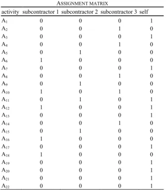
In this case we also have the following preferences. The functionality 1 should be designed (task A4) and

implemented (task A5) by the same subcontractors. The

same should be applied for functionality 2 and 3. Moreover the any two of functionalities should not to be designed or implemented by the same subcontractors. Also the tests for all functionalities (tasks A11, A12, A13, A14) should be done

TABLE IV ASSIGNMENT MATRIX

activity subcontractor 1 subcontractor 2 subcontractor 3 Self

A1 0 0 0 1

A2 0 1 0 0

A3 0 0 0 1

A4 0 0 1 0

A5 1 0 0 0

A6 0 1 0 0

A7 0 0 0 1

A8 0 0 1 0

A9 1 0 0 0

A10 0 1 0 0

A11 0 0 0 1

A12 0 0 0 1

A13 0 0 0 1

A14 0 0 1 0

A15 1 0 0 0

A16 0 1 0 0

A17 0 0 0 1

A18 1 0 0 0

A19 1 0 0 0

A20 1 0 0 0

A21 0 0 0 1

A22 0 0 0 1

With such a task distribution we obtain the total cost of the project K_C 161300$ and the total duration T_C 257 days. Finally, the total profits of the project equals 88700$.

Now let us consider the second of the models. In such case the values of elements in matrix X are given in Table I. Moreover in this model, we assume that each of the subcontractors reliably estimated the direct costs of the task. The times of duration (matrix T) and costs (matrix K) for tasks in project for all subcontractors are given in Table V and Table VI respectively. In both of these matrices we add our estimations of times and costs for tasks in project.

TABLE V THE TIME MATRIX

activity subcontractor 1 subcontractor 2 subcontractor 3 self

A1 7 0 0 14

A2 30 28 25 0

A3 14 0 0 14

A4 14 0 12 0

A5 10 5 0 0

A6 8 5 0 0

A7 30 0 0 14

A8 70 0 65 0

A9 52 40 0 0

A10 34 38 0 0

A11 7 0 10 10

A12 7 10 0 10

A13 7 10 0 10

A14 14 0 7 0

A15 14 14 0 0

A16 14 12 0 0

A17 21 14 0 30

A18 14 21 0 0

A19 5 0 0 14

A20 14 0 0 10

A21 7 0 0 7

A22 14 0 0 28

TABLE VI THE COST MATRIX

activity subcontractor 1 subcontractor 2 subcontractor 3 self

A1 2000 2000 2000 2000

A2 10000 10000 10000 10000

A3 3000 3000 3000 3000

A4 8000 8000 8000 8000

A5 8000 8000 8000 8000

A6 5000 5000 5000 5000

A7 1500 1500 1500 1500

A8 18000 18000 18000 18000

A9 15000 15000 15000 15000

A10 12500 12500 12500 12500

A11 4000 4000 4000 4000

A12 2500 2500 2500 2500

A13 2000 2000 2000 2000

A14 2000 2000 2000 2000

A15 2000 2000 2000 2000

A16 2000 2000 2000 2000

A17 5000 5000 5000 5000

A18 15000 15000 15000 15000

A19 20000 20000 20000 20000

A20 10000 10000 10000 10000

A21 5000 5000 5000 5000

A22 25000 25000 25000 25000

In this case also the preferences are exactly the same like in previous model. Moreover in this case we the vector of the profit margins and vector of ceiling prices for all task in the project. This information are given in Table VII and Table VIII respectively.

TABLE VII PROFIT MARGINS

subcontractor 1 subcontractor 2 subcontractor 3 self

30% 35% 40% 20%

TABLE VIII CEILING PRICES activity ceiling price

A1 3200

A2 16000

A3 4800

A4 12800

A5 12800

A6 8000

A7 2400

A8 28800

A9 24000

A10 20000

A11 6400

A12 4000

A13 3200

A14 3200

A15 3200

A16 3200

A17 8000

A18 24000

A19 32000

A20 16000

A21 8000

A22 40000

TABLE IV ASSIGNMENT MATRIX

activity subcontractor 1 subcontractor 2 subcontractor 3 self

A1 0 0 0 1

A2 0 0 1 0

A3 0 0 0 1

A4 0 0 1 0

A5 0 1 0 0

A6 1 0 0 0

A7 0 0 0 1

A8 0 0 1 0

A9 0 1 0 0

A10 1 0 1 0

A11 0 1 0 1

A12 1 0 0 1

A13 0 0 0 1

A14 0 0 1 0

A15 0 1 0 0

A16 1 0 0 0

A17 0 0 0 1

A18 1 0 0 0

A19 0 0 0 1

A20 0 0 0 1

A21 0 0 0 1

A22 0 0 0 1

With such a task distribution we obtain the total cost of the project KC 231050$ and the total duration TC 259 days. Finally, the total profits of the project equals 1850$.

IV. CONCLUSION

In this paper we consider two different contract types: the fixed price contract and the cost-plus contract. For both of this contract types we have presented a theoretical approaches for selecting subcontractors to develop selected tasks in the project. Even though the fact that each of the models relates to a completely different type of contact they are similar to each other. In the presented models, it is possible that such a division of labor is part of the job was done by the contractor itself and part by the subcontractor. Moreover, the presented models takes into account both preferences and constraints contracting authority in relation to the number and type of tasks that should be or cannot be done by one subcontractor. The usefulness of both of these models has been presented with an embodiment of the software development project. For this simple example we present the principle of each of the models and the differences between them. However, the exploration of the possibility of applying both of this models in real-life conditions requires further studies, both theoretical and practical on the basis of the real-life decision-making problems. The problem of optimal choice of the contract type (the fixed price contract or the cost-plus contract), according to the project environment and risk transfer policy, will be the subject of the future research.

REFERENCES [1] agilemanifesto.org (last access May 31th, 2013)

[2] Blaszczyk T., and Nowak B. (2008). “Project costs estimation on the basis of critical chain approach,” (in Polish), T. Trzaskalik (ed.): Modelowanie Preferencji a Ryzyko ’08, Akademia Ekonomiczna w Katowicach.

[3] Błaszczyk P., Błaszczyk T., Kania M.B., The bi-criterial approach to project cost and schedule buffers sizing, Lecture Notes in Economics and Mathematical Systems. New state of MCDM in the 21st century. Springer 2011, pp. 105-114.

[4] Goldratt E (1997) Critical Chain. North River Press.

[5] Gonzalez ,V., Alarcon L.F., Molenaar K. (2009). Multiobjective design of Work-In-Process buffer for scheduling repetitive projects. Automation in Construction 18, pp 95-108.

[6] Herroelen W, Leus R et al (2001) On the merits and pitfalls of critical chain scheduling. Journal of Operations Management 19:559-577. [7] Leach, L.(2003). Schedule and cost buffer sizing: how account for the

bias between project performance and your model. Project Management Journal 34 (2), pp. 34-47.

[8] PMI., 2008. A Guide to the Project Management Body of Knowledge (PMBOK® Guide) - Fourth Edition.

[9] Rogalska M, Bożejko W, Hejducki Z et al (2008) Time/cost optimization using hybrid evolutionary algorithm in construction project scheduling. Automation in Construction 18:24-31.

[10] Tukel O I, Rom W O, Eksioglu S D et al (2006) An investigation of buffer sizing techniques in critical chain scheduling. European Journal of Operational Research 172:401-416.

[11] Van de Vonder S, Demeulemeester E, Herroelen W, Leus R (2005) The use of buffers in project management: The trade-off between stability and makespan. International Journal of Production Economics 97:227-240.

[12] Van de Vonder S, Demeulemeester E, Herroelen W, (2007) A classification of predictive-reactive project scheduling procedures. Journal of Scheduling 10: 195-207.