FUNDAC
¸ ˜
AO GETULIO VARGAS
ESCOLA DE P ´
OS-GRADUAC
¸ ˜
AO EM ECONOMIA
Andr´
e Victor Doherty Luduvice
The life-cycle effects of social
security in a model with housing and
endogenous benefits
Andr´
e Victor Doherty Luduvice
The life-cycle effects of social
security in a model with housing and
endogenous benefits
Disserta¸c˜ao submetida a Escola de P´ os-Gradua¸c˜ao em Economia como requisito parcial para a obten¸c˜ao do grau de Mestre em Econo-mia.
´
Area de Concentra¸c˜ao: Desenvolvimento Econˆomico
Orientador: Pedro Cavalcanti Ferreira
Ficha catalográfica elaborada pela Biblioteca Mario Henrique Simonsen/FGV
Luduvice, André Victor Doherty
The life-cycle effects of social security in a model with housing and endogenous benefits / André Victor Doherty Luduvice. – 2014.
33 f.
Dissertação (mestrado) - Fundação Getulio Vargas, Escola de Pós- Graduação em Economia.
Orientador: Pedro Cavalcanti Ferreira. Inclui bibliografia.
1. Seguro social. 2. Habitação. 3. Bens de consumo duráveis. I. Ferreira, Pedro Cavalcanti. II. Fundação Getulio Vargas. Escola de Pós-Graduação em Economia. III. Título.
Agradecimentos
Agrade¸co primeiramente a Deus pela prote¸c˜ao durante toda essa jornada.
Ao meu orientador, Pedro Cavalcanti Ferreira, cuja confian¸ca em mim depositada e o debate de ideias foram os principais motores desse texto.
`
A Escola de P´os-Gradua¸c˜ao em Economia da Funda¸c˜ao Get´ulio Vargas e seus funcion´arios, pela oportunidade ´unica de estudo e pesquisa, pela s´olida forma¸c˜ao e por toda a estrutura necess´aria para o trabalho.
`
A Coordena¸c˜ao de Aperfei¸coamento de Pessoal de N´ıvel Superior (Capes) pelo apoio finan-ceiro para o programa de Mestrado em Economia.
Aos amigos antigos e aos amigos que aqui fiz. Os primeiros pelo companheirismo de sempre e os ´ultimos por terem proporciondo, em aprendizado e vivˆencia, inesquec´ıveis dois anos e meio.
`
“ ‘Cheshire Puss’, she began, rather timidly, as she did not at all know whether it would like the name: however, it only grinned a little wider. ‘Come, it’s pleased so far’, thought Alice,
and she went on. ‘Would you tell me, please, which way I ought go from here?’
‘That depends a good deal on where you want to get to’, said the Cat.
‘I don’t much care where–’ said Alice.
‘Then it doesn’t matter which way you go,’ said the Cat.
‘– so long as I get somewhere,’ Alice added as an explanation.
‘Oh, you’re sure to do that’, said the Cat, ‘if you only walk long enough.’ ”
Resumo
Esse artigo desenvolve um modelo de equil´ıbrio geral com gera¸c˜oes sobrepostas e agentes heterogˆeneos que realizam escolhas de consumo de bens n˜ao dur´aveis, inves-timento em im´oveis para moradia e de oferta de trabalho. A partir de uma idade determinada, os agentes se aposentam e recebem benef´ıcios da seguridade social que s˜ao dependentes dos rendimentos passados. O modelo ´e calibrado, solucionado numericamente e ´e capaz de gerar estat´ısticas agregadas similares `as dos EUA e tamb´em de gerar perfis m´edios de ciclo da vida das vari´aveis de decis˜ao consistentes com os dados e a literatura. ´E tamb´em conduzido um exerc´ıcio em que se elimina completamente o sistema de seguridade social e s˜ao feitas compara¸c˜oes com o modelo original. Os resultados nos permitem evidenciar a importˆancia da endogeneidade da oferta de trabalho e dos benef´ıcios para o comportamento suavizador de consumo dos agentes.
Palavras-chave: Seguro social. Habita¸c˜ao. Bens de consumo dur´aveis.
Abstract
This article develops a life-cycle general equilibrium model with heterogeneous agents who make choices of nondurables consumption, investment in homeowned housing and labour supply. Agents retire from an specific age and receive Social Security benefits which are dependant on average past earnings. The model is calibrated, numerically solved and is able to match stylized U.S. aggregate statistics and to generate average life-cycle profiles of its decision variables consistent with data and literature. We also conduct an exercise of complete elimination of the Social Security system and compare its results with the benchmark economy. The results enable us to emphasize the importance of endogenous labour supply and benefits for agents’ consumption-smoothing behaviour.
Contents
1 Introduction 11
2 Literature Review 12
3 The Model 15
3.1 Environment . . . 15
3.1.1 Demography . . . 15
3.1.2 Preferences . . . 15
3.1.3 Technology . . . 16
3.1.4 Timing . . . 16
3.1.5 Housing Market Transaction Costs . . . 17
3.1.6 Individual’s Budget Constraint . . . 17
3.1.7 Government . . . 18
3.2 Household’s Problem . . . 19
3.3 Equilibrium . . . 19
4 Calibration 21 4.1 Demography . . . 21
4.2 Preferences and Technology . . . 21
4.3 Individual Labour Productivity . . . 22
4.4 Social Security and Taxation . . . 23
4.5 Transaction Costs . . . 23
5 Results 25 5.1 Benchmark Economy . . . 25
5.2 Counterfactual Exercise: Elimination of Social Security . . . 27
6 Conclusions 31
List of Figures
5.1 Average households’ allocation decisions over the life cycle. . . 26
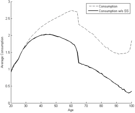
5.2 Average households’ consumption over the life cycle. . . 28
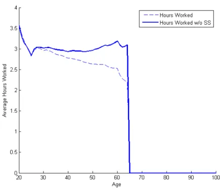
5.3 Average households’ hours worked over the life cycle. . . 29
5.4 Average households’ asset accumulation over the life cycle.. . . 30
List of Tables
4.1 Parameter values for the economies simulated . . . 24
5.1 Quantitative properties of the benchmark economy. . . 25
Chapter 1
Introduction
The decision of consumption of durable goods is of major importance in the life-cycle of agents, specially when connected to the decision of portfolio allocation in its beginning (Villaverde and Krueger,2010). Housing is viewed by agents as a durable good and it is the one that constitutes the largest share of most homewowners’ total assets. What are the impacts of Social Security and its mandatory savings in individuals’ portfolio throughout life? Moreover, how does the hours worked in early ages impact investment in housing and future consumption during retirement? In order to address such questions we develop and numerically solve an overlapping genera-tions dynamic general equilibrium model with heterogeneous agents. In our model, individuals’ make decisions on nondurables consumption, investment in homeowned housing and labour supply. From an specific realistic age, agents retire, leave the labour force and receive Social Security benefits. The Social Security system is modelled in a manner that past earnings in-fluences households’ contribution and its future benefits. Also, in our model, individuals face transaction costs when changing housing stock.
Our setting is part of a literature connected to the studies ofYang(2009),Chen(2010), Fer-reira and Santos(2013) and others that are later thoroughly discussed. We conduct an exercise where we completely eliminate the Social Security system of the benchmark economy and com-pare the different outcomes. The model is able to closely match aggregate statistics of the U.S. and also the life-cycle profiles of nondurables consumption, housing investment and asset accu-mulation present in the literature and data. We are able to find that endogenous labour-supply and the presence of the endogenous benefits are key features to understand the smooth decline of expenditure in nondurables in later ages by agents. When Social Security is eliminated, the adjustment in hours worked is used to finance asset accumulation for consumption smoothing in retirement.
Chapter 2
Literature Review
One of the first papers of the literature that models a dynamic general equilibrium with over-lapping generations and social security is the one from Huggett (1996). It is a pioneer paper assessing wealth distribution issues and it carries two main modifications of the OLG classics: presence of earnings and lifetime uncertainty and the absence of markets for issuing it. Also, the model provides us a very rich framework allowing for complex features such as retirement, precautionary and lifetime uncertainty saving motives.
The economies simulated by Huggett (1996) are capable of generating the US wealth Gini coefficient. However, the model economies do such by generating a high fraction of zero and negative wealth-holders and not by concentrating wealth in the extreme upper tail of the dis-tribution. The simple intuition for this fact is that there are no multi-millionaires in a model in which all agents within an age group hold the same wealth. The addition of earnings inequality improves the match for the top 20%, but account for little less than half of the wealth held by the top 1%. A key feature is that the fraction of agents with zero or negative wealth is above US levels even when debt is not allowed. In frameworks in this Aiyagari’s fashion few agents tend to be exactly at the corner of the borrowing constraint. Thus, life-cycle considerations seem to be important for generating low wealth levels.
Models that followed this tradition introduced by Huggett(1996) are usually based on the ones by Huggett and Ventura (1999) and Conesa and Krueger (1999), where the environment first introduced is amplified for a more complex Social Security system. It is a system where benefits are a function of past earnings which is more close to reality and allows the comparison of different proposed designs of social security systems. The way we calculate Social Security benefits in our model is strongly inspired in the framework by Huggett and Ventura (1999) which became a benchmark in the literature.
benchmarks needed for the understanding of the study we conduct in this article: empirically, both durables and nondurables follow a hump-shaped pattern over the life cycle and, quan-titatively, the intrinsic characteristics of durables leads to its accumulation in early-life and subsequent substitution by nondurables consumption and allocation of the portfolio in financial assets.
One natural development arising from the literature of durables consumption is the consump-tion of housing service flows.Yang(2009) introduces this issue in a dynamic general equilibrium framework in a OLG environment but with no social security. As micro data show different paths for consumption of housing and nonhousing goods, it is of interest to understand how those paths are related to consumption and asset allocation. Nonhousing shows a hump-shaped traditional pattern in life-cycle profile but housing shows an increase in early years and the paper is able to replicate closely the pattern present in the data. Two features ofYang(2009)’s model that helped the match to happen were the explicit modelling of collateral restrictions and of transactions costs. Borrowing difficulties in the early age influence agents to invest in housing and the costs of leaving home for homeowners explain why no further house investments are made in old age.
The author proposes a model with two different types of consumers of housing, the home-owners, which accumulate stock and the renters, which consume its service flows. Households borrow early in life to buy houses and thus save in this fashion. As agents age, the profile of financial assets and housing tend to intersect as they increase their holding of financial assets and housing services are already accumulated. The model we propose was strongly inspired in
Yang (2009) framework. However, the possibility of housing tenure choice is not yet present in our setting although we recognize it as natural future extension.
Nevertheless, a crucial aspect related to the savings decision of agents is the presence of a social security system present in the economy. Social security discourage household savings and redistributes resources from one’s working years to retirement. Chen (2010) extends the
Yang(2009)’s framework in order to include a social security system with benefits independent from earnings. Also, the author includes housing market frictions which connects the model to reality such as the greater depreciation of rented housing due to moral hazard issues.
The author finds that both housing quantities and homeownership are affected by the elim-ination of social security and that the aggregate impacts of such policy reform is significantly larger in economies with housing than with those with only non-durable consumption. The mechanism behind this aggregate consequence is the substitution effect arising from the change in the interest rate after the elimination of the social security system.
The mechanism of such elimination suggested byChen (2010) is as follows: the elimination of social security reduces interest rates as it drives households to savings in assets. This change in the interest rate lowers the price of housing causing a substitution effect in between the two types of consumption. There is then an increase in the housing stock which leads to a large capital-output ratio. This is the key channel not provided by an economy with only the riskless financial asset and nondurable consumption like the present in Huggett and Ventura(1999).
the composition of its permanent wealth and alter their decision to dedicate more time to work and enlarge labour income. Also, the Social Security system designed by Chen (2010) is the simplest possible and does not account for the possibilities once opened in the seminal approach by Huggett and Ventura (1999). Therefore, we inspire ourselves in Ferreira and Santos(2013) who studies such a type of economy where individuals have endogenous labour supply and optimally pick the time to leave the labour force and to retire. The authors are able to match the retirement profile of the U.S. economy and to reproduce differences in heterogeneities arising from productivity and health status differences.
In Ferreira and Santos (2013), the analysis of the evolution of the retirement choices of agents between 1950 and 2000 shows that most of the changes in the retirement profile are due to the changes in Social Security and the introduction of the Medicare program. The authors are able to match the peak of Social Security applications ate the age of 62 and assess that the isolated effect of longevity would be a delay in leaving the labour force and thus cannot explain the decrease of the presence of the elderly in the labour force.
Chapter 3
The Model
3.1
Environment
3.1.1 Demography
The economy is populated by a continuum of mass one agents who live at mostT periods. Time j is discrete and the economy has an infinite horizon. There is an uncertainty regarding the time of death in every aget= 1, . . . , T so that the individual faces probabilityψtof surviving to
aget. Therefore, in very period, a fraction of the population dies and leaves accidental bequests which are assumed to be distributed equally among all surviving individuals. The age profile of the population {µt}Tt=1 is modelled by assuming that the fraction of agents at age t in the
population is given by law of motionµt= (1+ψtgn)µt−1, that satisfies
PT
t=1µt = 1 and where gn
is the population growth rate.
3.1.2 Preferences
Households enter in the economy without assets and are endowed with ¯l units of time for everyt. In each period of life, the individuals maximizes their discounted expected utility from nondurable goods consumption ct, housing service flows consumption, ht, and leisure, (¯l−lt).
The lifetime utility function is:
E
" T X
t=1
βt−1
t Y
k=1
ψk !
u(ct, ht,¯l−lt) #
(3.1)
where β is the discount factor and E is the expectation operator. The instant utility is assumed to take the form:
u(ct, ht,¯l−lt) =
[˜cρt(¯l−lt)1−ρ]1−γ
1−γ (3.2)
where
˜
ct= ((1−ν)cθt +νhθt) 1
θ (3.3)
in the consumption bundle andρ is the share of consumption of nondurables and housing, ˜c, in the agent’s instant utility.
3.1.3 Technology
There is only one type of good produced in this economy whose technology is given by a Cobb-Douglas production function with constant returns to scale: Y =KαN1−α, whereα∈(0,1) is
the output share of capital income andY,K and N denote, respectively, the aggregate output, aggregate physical capital and aggregate hours worked. The output can be consumed, invested in physical capital or invested in housing, H, on a one-to-one basis.
The price of the nondurable goods is normalized to one and aggregate investment in physical capital,Ik, is given by the following law of motion whereδk is its depreciation rate:
Ik=K′−(1−δk)K (3.4)
.
On the other hand, the aggregate investment in housing, Ih, consists only of homeowned
housing capital. It follows a standard law of motion whereδh is the depreciation rate:
Ih=H′−(1−δh)H (3.5)
.
This technology is used by a representative firm that behaves competitively maximizing profits while choosing labour and capital with given prices. The profit maximization problem is:
Π = max
K,N K
αN1−α−wN−(r+δk)K. (3.6)
The first-order conditions of the problem are:
r =α
K N
α−1
−δk (3.7)
w= (1−α)
K N α (3.8) . 3.1.4 Timing
capital depreciates. Uncertainty about early death is revealed and all information is publicly observed. Accidental bequests are distributed.
3.1.5 Housing Market Transaction Costs
Housing is fixed in space and has a considerable degree of heterogeneity. Buyers and sellers spend time and resources when buying specific housing units. Also, for a homeowner, opportunity costs of time associated with every kind of search when moving need to be taken into account in the decision of agents.
Therefore, we will consider a nonconvex transaction cost τ(ht, ht+1) that the homeowner
incurs each time she changes housing stock holdings. The specification of the transaction cost follows Chen(2010) and is set asτ(h, ht+1) =✶ht+1ϕht, where
✶ht+1
1, ifht+16=ht
0, ifht+1=ht
(3.9)
and ϕ is a parameter that maps the transaction cost into a fraction of the selling value of the house.
3.1.6 Individual’s Budget Constraint
In this economy, individuals make decisions about asset accumulation, housing purchases and labour supply. As the labour supply is endogenous we will follow Ferreira and Santos (2013) and consider that individuals are in the labour force if they supply at least 5% of their time endowment ¯l.
As individuals supply labour, they earn a wage w and are submitted to idiosyncratic pro-ductivity shocks z. We denotee(z, t) the efficiency index of an agent with agetand shock zso that the labour earnings arewlte(z, t), whereltis the labour supply. Individuals are allowed to
leave and enter the labour force whenever they want before retiring and receiving their social security benefits. The retiring age is absorbing and all individuals are automatically shut down from the labour force once they reach it.
The efficiency index is described by e(z, t) = ηtz, where ηt is a deterministic age-specific
component and z is the shock to the efficiency units of labour z ∈ Z = {z1, . . . , zi}, where i
is to be later calibrated. The shock follows a Markov process with transition matrix πz,z′ = Pr(zt+1 =z′|zt=z) and stationary distribution Π(z) = Pr(zt=z). From Tr and onwards the
labour efficiency is zero (z= 0) and agents live off their benefits and their accumulated wealth. All workers in the economy pay labour income tax τSS which is collected by the government
to finance the Social Security’s benefit payment to the retired agents. Therefore, the earnings of a worker at age tare:
yt= (1−τSS)wlte(z, t)
.
order to protect themselves from labour income uncertainty. Also,htstands for the homeowner
housing purchases.
We denote x individual average lifetime earnings. The average of lifetime earnings is calcu-lated by taking into account individual earnings up to age Tr. The law of motion of x is:
xt=
xt−1∗(t−2) + min{wlte(z, t−1), ymax}
t−1 , t= 2, . . . , Tr. (3.10) The benefits that the agents receive during retirement are endogenous and depend on the average lifetime earnings. The function b(xt) describes the benefit that agents are entitled to
at the retirement age. It is a piecewise linear function specified in accordance with U.S. social security system rules:
b(x) =
θ1x, ifx≤y1
θ1y1+θ2(x−y1), ify1< x≤y2
θ1y1+θ2(y2−y1) +θ3(x−y2), ify2< x≤ymax
(3.11)
where 0≤θ3 < θ2< θ1 and (y1, y2, y3) are the bend points of the function.
Therefore, up to an average earnings level of y1 retired agents are entitled to θ1 so that θ1
corresponds to the replacement rate. If the average of past earnings are greater than y1 but
smaller thany2, they will earnθ1y1+θ2(x−y1). The other step of the function is interpreted in
similar manner only differing by the fact that there is a limit for the creditable income denoted by ymax. For values above it, all individuals receive the highest amount of benefits possible in
social security system.
The budget constraint of an agent until age t=Tr−1 will then be:
at+1+ht+1 = (1 +r)at+ (1−δh)ht+yt−τ(ht, ht+1) +ξ−ct. (3.12)
For ages t=Tr, . . . , T, it becomes:
at+1+ht+1= (1 +r)at+ (1−δh)ht+b(x)−τ(ht, ht+1) +ξ−ct. (3.13)
We assume that there is no altruistic bequest motive and, as there is the certainty of death atT+ 1, agents alive at age T consume all resources implyingaT+1 = 0.
3.1.7 Government
In our economy, there is a government which manages the Social Security system. It distributes pension benefitsb(x) to pensioners financing it with the collection of the exogenous taxτSS from
household’s labour income. We will assume also that the government expends G in order to balance eventual deficits in the social security budget. Thus, the government budget is described by the following equation:
G=τSSwN−B (3.14)
Moreover, the government is also responsible for collecting all accidental bequests and trans-fering it to all agents on a lump-sum basis throughξ in the way already described.
3.2
Household’s Problem
Let Vw,t(st) denote the value function of a t year old agent, where st = (at, ht, xt, zt) ∈ S is
the individual state space and let Vss,t(st) for t = Tr, . . . , T denote the value function of an
individual aged t who is out of the labour force and is receiving Social Security benefits. We also set the value function of the terminalT to zero,Vss,T+1(st+1) = 0.
The problem of an agent with aget= 1, . . . , Tr−1 is represented in the following recursive
form:
Vw,t(s) = max c,l,a′,h′
u(c, h′,¯l−l) +βψ
t+1EVw,t+1(a′, h′, x′, z′) (3.15)
subject to
c+a′+h′ = (1 +r)a+ (1−δh)h+y−τ(h, h′) +ξ a′ ≥0, c≥0, 0≤l≤¯l, h′ ≥0.
For individuals at ages t=Tr, . . . , T the problem is:
Vss,t(s) = max c,a′,h′
u(c, h′,¯l) +βψ
t+1E
Vss,t+1(a′, h′, x′, z′) (3.16)
subject to
c+a′+h′= (1 +r)a+ (1−δh)h+b(x)−τ(h, h′) +ξ a′ ≥0, c≥0, h′ ≥0.
The solution of the dynamic programs (15) and (16) provides us the decision rules for the asset holdingsda,t:S →R++, consumption dc,t:S →R++, labour supply dl,t:S →[0,¯l] and
housing purchasesdh,t :S→R++.
3.3
Equilibrium
Agents are heterogeneous at each point in time both in the agetdimension and in the states∈S. The agents’ distribution at age t among the states s is described by a measure of probability λt defined on subsets of the state space S. Let (S,Ω(S), λt) be a space of probability where
Ω(S) is the Borelσ-algebra onS. For eachω⊂Ω(S),λt(ω) denotes the fraction of agents aged
t that are in ω. There is a transition function Qt(s, ω) which governs the transition from age
t to age t+ 1 and that depends both of the stochastic process for z and on the decision rules obtained from the household’s problem.
Definition Given the policy parameters, a recursive competitive equilibrium for this econ-omy is an allocation of value functions {Vw,t(s), Vss,t(s)}, policy functions for individual asset
dh,t(s), prices {w, r}, age-dependent but time-invariant measures of agents λt(s), transfers ξ
and tax on labour earningsτSS such that:
1. {da,t(s), dc,t(s), dh,t(s), dl,t(s)}solve the dynamic problems (15) and (16);
2. The individual and aggregate behaviours are consistent:
K = T X t=1 µt Z S
dat(s)dλt
H= T X t=1 µt Z S
dh,t(s)dλt
C= T X t=1 µt Z S
dc,t(s)dλt
N =
Tr−1
X
t=1
µt Z
S
dl,t(s)e(zt, t)dλt
T C=
T X t=1 µt Z S
τ(ht, ht+1)(s)dλt
3. {w, r} are such that they satisfy the firm first-order conditions (7) and (8);
4. The final good market clears:
T X t=1 µt Z S
{dc,t(s)+[da,t(s)−(1−δk)da,t−1(s)]+[dh,t(s)−(1−δh)dh,t−1(s)]}+T C =KαN1−α
5. Given the decision rules,λt(ω) satisfies the following law of motion:
λt+1(ω) = Z
S
Qt(s, ω)dλt, ∀ω⊂Ω(S)
6. The distribution of accidental bequests equals the savings left from dead households:
ξ =
T X
t=1
µt(1−ψt+1) Z
S
[da,t(s) +dh,t(s)]dλt
7. Government budget balances:
G=τSSwN−
T X
t=Tr µt
Z
S
Chapter 4
Calibration
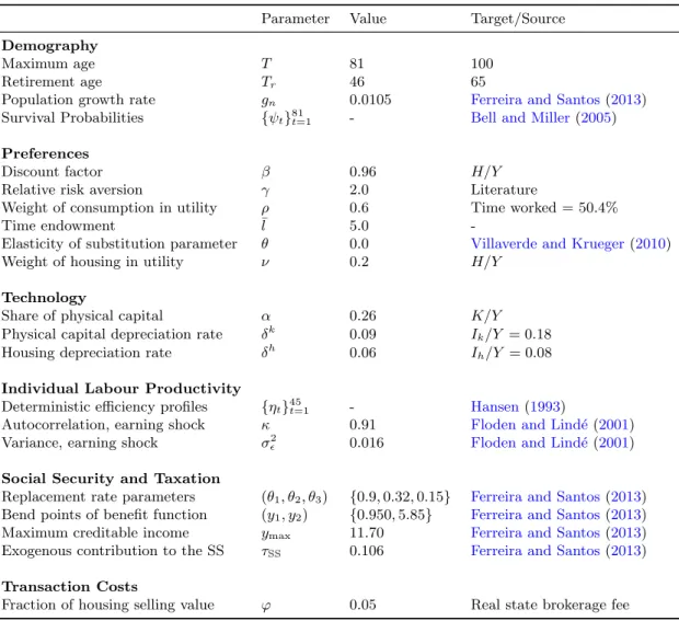
In this section we describe our calibration procedure. Our focus and references are all directed to match targets for the U.S. economy. The details of the algorithm and computation of the nu-merical solution are described in the Appendix A. At the end of the section, Table 1 summarizes all the information regarding the parameters calibrated.
4.1
Demography
One period in our model corresponds to one year of calendar time. The population age profile
{µt}Tt=1 depends on the population growth rate gn, the survival probabilities ψt and the
max-imum age T. We will allow agents to live until T = 81 years old. We map it into an economy where agents are born with age 20 which makes the real maximum age 100 years. Also, agents face compulsory retirement at Tr = 46 which stands for age 65 in reality.
The survival probabilities {ψt}81t=1 are taken from Bell and Miller (2005). The population
growth rate is chosen so that the age distribution in the model replicates the dependency ratio observed in the data. We use the calculation present Ferreira and Santos (2013) which is gn= 0.0105.
4.2
Preferences and Technology
We set the coefficient of relative risk aversion γ to be 2 which is a well-known benchmark in macroeconomic literature. The parameter governing the elasticity of substitution between the consumption of nondurables and housing durables θ is studied by Villaverde and Krueger
(2010) and, based in several empirical studies, they argue that the hypothesis ofθ= 0 cannot be rejected at a low significance level. We will use their calibration which implies a unit elasticity of substitution between the two sorts of consumption and a Cobb-Douglas format with parameter ν ∈(0,1).
use as reference for the targets include rented housing capital alongside with the homeowned one. Due to the fact that in the National Accounts tradition all housing capital is aggregated in imputed value, there is no loss of generality in using the same targets for our model composed solely of owner-occupied housing.
We setα = 0.26 so that the share of physical capitalK income in outputY matches the one from the literature. As we do not consider productivity growth in our model, the depreciation rates δi, i = {K, H}, can be obtained with the formula δi = Ii/Y
i/Y . The depreciaton rate of
physical capital is set as δk = 0.09 to yield an investment in physical capital to output ratio Ik/Y = 0.18. The share of housing consumption in the utility ν and the parameter β are
jointly calibrated to yield aH/Y in accordance with the literature. They are then,ν= 0.2 and β = 0.965. TargetingIh/Y = 0.08, in accordance with Iacoviello and Pavan (2013), we set the
depreciation of the housing capital asδh = 0.06. The interest rate implied by our calibration is
r=αKY −δk= 0.0330 at the initial steady state.
The parameters ¯l and ρ which govern the time spent working by agents are, as stated inFerreira and Santos(2013), difficult to be calibrated in overlapping generations models with heterogeneous agents. There is not a one-to-one relation of the parameterρto hours worked as in simpler representative agents models. The empirical evidence suggests a value of approximately of 30% to be the fraction of time individuals spend working. In their seminal paper which, does not consider durables consumption,Huggett and Ventura(1999) chooseρ= 0.33 and are able to obtain an average of 31% to 32% of hours devoted to work. InIacoviello and Pavan(2013), one of the few papers in the literature similar to ours but with separable utility, authors calibrate these parameters so that time spent working is 40%. To our numerical analysis, we chose one of the calibrations that was the most stable for computation and that did not compromised the other targets, ¯l= 5.0 and ρ = 0.6. This yields us a fraction of 50,4% of time spent working of the total endowment of time available.
4.3
Individual Labour Productivity
The deterministic age profiles of labour productivity{ηt}45t=1 are taken fromHansen(1993). We
followChen(2010) in parametrizing the idiosyncratic component of the labour-income process. He uses the AR(1) suggested byHuggett(1996) for the log of the shock:
logzt+1=κlogzt+ǫt (4.1)
where ǫt∼ N(0, σ2ǫ). Floden and Lind´e(2001) use PSID data to estimate and AR(1) process
which is similar to the one above. We use their findings to set the auto-regressive coefficientκ and the variance of the innovationσ2
ǫ as 0.91 and 0.016, respectively. Using the method present
4.4
Social Security and Taxation
The parametrization of the benefit function is held by the specification of the parameters
{θ1, θ2, θ3, y1, y2, ymax}. We follow Ferreira and Santos (2013) as they have, to the extent of
our knowledge, the most recent calibration procedure for such parameters. They determine the bend points {y1, y2} and the replacement rates associated (governed by{θ1, θ2, θ3}), based on
the formula of the calculation of the primary insurance amount (PIA).
As we calibrate the demography of our economy almost in the same way that Ferreira and Santos (2013) calibrate their economy for the year 2000, we will use the same parameters obtained by them for this year. We then maintain the same setting of the parameters which are on percentage, i.e., θ1 = 0.9,θ2 = 0.32 and θ3 = 0.15. The bend points and the maximum
income creditable are calculated by the authors targeting variables which are in level values based on a time endowment set to be ¯l= 1. Therefore, we need to adjust those parameters to our economy multiplying them by 5. This yields us y1 = 0.950, y2 = 5.85 and ymax = 11.70.
Finally, we follow the authors and set the exogenous contribution from workers to Social Security system, τSS, as 10.6% of their labour income.
4.5
Transaction Costs
As stated previously the transaction cost function for selling housing is τ(ht, ht+1) =Iht+1ϕht.
Table 4.1: Parameter values for the economies simulated
Parameter Value Target/Source
Demography
Maximum age T 81 100
Retirement age Tr 46 65
Population growth rate gn 0.0105 Ferreira and Santos(2013)
Survival Probabilities {ψt}81t=1 - Bell and Miller(2005)
Preferences
Discount factor β 0.96 H/Y
Relative risk aversion γ 2.0 Literature
Weight of consumption in utility ρ 0.6 Time worked = 50.4%
Time endowment ¯l 5.0
-Elasticity of substitution parameter θ 0.0 Villaverde and Krueger(2010)
Weight of housing in utility ν 0.2 H/Y
Technology
Share of physical capital α 0.26 K/Y
Physical capital depreciation rate δk
0.09 Ik/Y = 0.18
Housing depreciation rate δh
0.06 Ih/Y = 0.08
Individual Labour Productivity
Deterministic efficiency profiles {ηt}45t=1 - Hansen(1993)
Autocorrelation, earning shock κ 0.91 Floden and Lind´e(2001)
Variance, earning shock σ2
ǫ 0.016 Floden and Lind´e(2001)
Social Security and Taxation
Replacement rate parameters (θ1, θ2, θ3) {0.9,0.32,0.15} Ferreira and Santos(2013)
Bend points of benefit function (y1, y2) {0.950,5.85} Ferreira and Santos(2013)
Maximum creditable income ymax 11.70 Ferreira and Santos(2013)
Exogenous contribution to the SS τSS 0.106 Ferreira and Santos(2013)
Transaction Costs
Chapter 5
Results
This section summarizes some of the results obtained in the numerical solution of the model. We first show results for the benchmark economy. Subsequently, we show how this economy answers to a counterfactual exercise where we completely eliminate the Social Security system but maintain the benchmark calibration.
Our focus are in the measures of the aggregate variables and ratios and in the average life-cycle profiles of individuals’ decisions. Up to this moment, we have not conducted the exercise of simulating the economy for a large number of agents. In a model with huge computational costs like ours, such time-consuming exercise was not yet feasible and thus we are not able to provide calculations for Gini coefficients of key aggregate variables.
5.1
Benchmark Economy
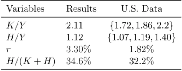
Table 2 below shows results for the aggregate variables and ratios of main interest. All the num-bers present in the column named “U.S. Data”, unless elsewhere noticed, are target calculations taken from articles in the literature of overlapping generations models with heterogeneous agents and housing.
Table 5.1: Quantitative properties of the benchmark economy.
Variables Results U.S. Data
K/Y 2.11 {1.72,1.86,2.2}
H/Y 1.12 {1.07,1.19,1.40}
r 3.30% 1.82%
H/(K+H) 34.6% 32.2%
We are able to obtain a capital to output ratio and a housing to output ratio values within the range of the U.S. data provided by the literature. As already stated, such models also consider rented housing capital and therefore slight differences from our estimation are understood not to be compromising. As we chose our depreciation rate of physical capital in order to match Ik/Y = 0.18, the implied interest rate r after targeting K/Y is high when compared to the
The ratio H/(K +H) is the share of housing in the total net worth and it is a non-targeted variable. As the table shows, our model is able to closely replicate the share’s value for the U.S. data.
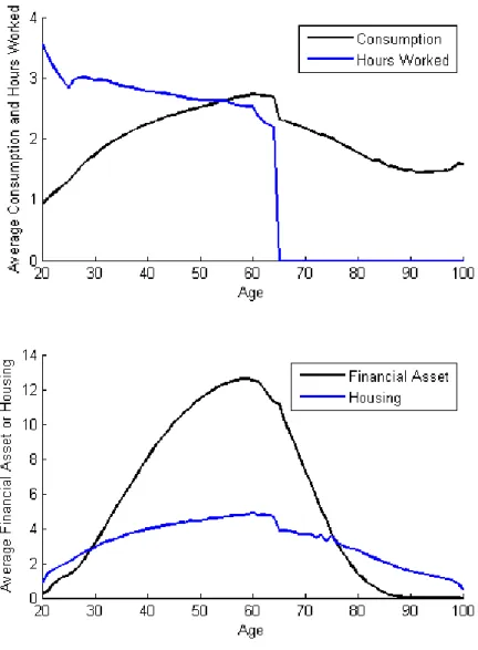
Figure 5.1: Average households’ allocation decisions over the life cycle.
Figure 1 show graphs of the average life-cycle profiles of non-housing and housing consump-tion, asset allocation and hours worked. All of the profiles we find show consistency with the ones present in the literature. In the first graph, we are able to see that the expenditures in nondurables consumption have a hump-shaped life-cycle pattern with peak in age 60. This shape, as observed by Villaverde and Krueger (2010), emerges by the fact that, early in life, housing durables generates service flows and it is therefore optimal to agents to compromise nondurables consumption and build-up a stock of housing. Later, as this stock gets higher, the marginal utility of non-housing consumption also gets higher and substitution effects emerge.
rates and agents sharply decline their consumption when labour income is not available (Yang,
2009). Due to the fact that our model presents endogenous retirement benefits, agents are able to increase hours devoted to work to guarantee higher benefits in the future and smooth consumption in old ages. This is supported by the fact that, in our model, the average hours worked are higher in early life and before retirement when compared with other models with endogenous labour supply (Huggett and Ventura,1999;Ferreira and Santos,2013).
Analysis of the portfolio allocation in the life-cycle in the second graph shows that in the beginning of life, agents save in housing as it provides service flows in the future. From age 30 and onwards the dominant asset in the portfolio is then changed to the financial asset which is accumulated until retirement to finance primarily nonhousing consumption. As for the investment in housing, we observe a peak between 50 and the retirement age followed by a slow downsize later in life. This replicates well the empirical facts provided byYang (2009) and also show, when compared with the assets curve, the important role played by the transaction costs in generating the life-cycle smoothness of this profile.
Comparing with the portfolio profiles of the literature, agents in our model accumulate more financial assets in early ages showing a concave pattern of the curve before retirement. This is consistent with the data present in Villaverde and Krueger (2010) and contrasts with the shape obtained both by these authors and byChen(2010), which is slightly convex. One of the possible explanations for this match is the fact that, in our model, agents are able to adjust their hours worked which are summed up with the service flows obtained from early-bought housing. This allows them to overaccumulate assets both by precautionary and consumption-smoothing motives.
5.2
Counterfactual Exercise: Elimination of Social Security
Following Chen (2010), we conduct a counterfactual exercise with the no-credit economy in which we completely eliminate the Social Security structure of the model. Such experiment provides us some intuition about potential long-run effects of changes in the Social Security policy and what are agents’ responses towards the private means of accumulating savings for retirement.
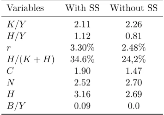
Table 5.2: Aggregate effects of eliminating Social Security.
Variables With SS Without SS
K/Y 2.11 2.26
H/Y 1.12 0.81
r 3.30% 2.48%
H/(K+H) 34.6% 24,2%
C 1.90 1.47
N 2.52 2.70
H 3.16 2.69
As shown in Table 3, eliminating Social Security, whose benefits share in output B/Y was only 9%, has major impacts on housing in the simulated economies. The decrease in the total of housing accumulated is of 14.8%. The capital to output ratio stays almost the same, however,H/Y decreased 27.6% from its value in the benchmark economy. Also, the interest rate decreased 24.8%, which could be partially accounting for the increase in K/Y. Following the same direction, the share of housing in net worth also decreases considerably. Furthermore, the aggregate expenditure in nondurable consumption decreases 22.6% and the total hours worked increased by almost 7.1%.
Figure 5.2: Average households’ consumption over the life cycle.
In Figures 2 to 5 we see the comparison between the average profiles of the individuals’ decisions over the life cycle. In Figure 2 there is an abrupt reduction in the nonhousing con-sumption expenditure and that it shows a more pronounced hump-shaped pattern with a solid decrease after retirement. This goes in accordance with the analysis stated previously of the importance of social security benefits in consumption smoothness.
By looking at Figure 3, and, also taking into account the aggregate result, we note that the individuals increase their average hours worked sustaining it on a high average level until the last moment before retirement. There is now more incentive to work as agents need to finance greater asset accumulation in early ages to insurance against future idiosyncratic shocks and finance consumption in retirement. Also remarkable is that, although agents lost one of their channels of incentive to work, the endogenous benefits, the need to smooth consumption in an economy without future social insurance overcomes this loss and provokes the rise in hours worked.
Figure 5.3: Average households’ hours worked over the life cycle.
Figure 5.4: Average households’ asset accumulation over the life cycle.
Chapter 6
Conclusions
In this paper we have proposed and numerically solved an overlapping generations model with heterogeneous agents where individuals make choices of nondurables consumption, investment in homeowned housing and labour supply. Also, in our model, individuals face transaction costs when changing housing stock, there is a Social Security system in which benefits are dependent on agents’ average past earnings and retirement is an absorbing state beginning in a realistic age. The model matches closely some of the aggregate statistics of the U.S. economy as well as the life-cycle profile of the decision variables studied.
The results for the benchmark economy show us that adjustments in the labour supply in order to finance higher benefits are crucial to generate a smooth reduction in the expenditure in nondurables after retirement, a fact observed in the data. Also, the same possibility of increasing the hours worked in youth, and thus labour income, allows individuals to overaccumulate assets and exhibit a concave curve in early ages in their average financial savings profile.
Furthermore, in an exercise where the Social Security is eliminated in the economy, our model shows that the increase in the average hours worked plays an important role in increasing savings in assets which will be the major source of wealth for agents in their retirement. Also, as inChen (2010), the interest rate channel continues to be the major mechanism through which individuals allocate financial assets and housing in their portfolio.
Finally, there are many possibilities of amplifying our model to settings that would be able to account for a broader research agenda. The first natural modification is to follow Yang
(2009) and Chen (2010) and numerically solve an economy where individuals make housing tenure choices where it would be possible to study the housing market for renters. Also, as in
Bibliography
Bell, F. and M. Miller (2005). Life table for the united states social security area 1900-2100.
Office of the Chief Actuary, Social Security Administration, Actuarial Studies 116.
Chen, K. (2010). A life-cycle analysis of social security with housing. Review of Economic Dynamics 13, 597–615.
Conesa, J. C. and D. Krueger (1999). Social security reform with heterogeneous agents. Review of Economic Dynamics 2, 757–795.
Ferreira, P. C. and M. R. Santos (2013). The effect of social security, health, demography and technology on retirement. Review of Economic Dynamics 16, 350–370.
Floden, M. and J. Lind´e (2001). Idiosyncratic risk in the united states and sweden: is there a role for government insurance? Review of Economic Dynamics 4, 406–437.
Guerrieri, V. and G. Lorenzoni (2012). Credit crises, precautionary savings, and the liquidity trap. Working Paper.
Hansen, G. (1993). The cyclical and secular behaviour of the labour input: Comparing efficiency units and hours worked. Journal of Applied Econometrics 8, 71–80.
Huggett, M. (1996). Wealth distribution in life-cycle economies. Journal of Monetary Eco-nomics 38, 469–494.
Huggett, M. and G. Ventura (1999). On the distributional effects of social security reform.
Review of Economic Dynamics 2, 498–531.
Iacoviello, M. and M. Pavan (2013). Housing and debt over the life cycle and over the business cycle. Journal of Monetary Economics 60, 221–238.
Press, W., S. Teukolsky, W. Vetterling, and B. Flannery (1994). Numerical Recipes in Fortran: The Art of Scientific Computing (2nd Edition ed.). Cambridge University Press.
Tauchen, G. (1986). Finite state markov chain approximations to univariate and vector autore-gression. Economic Letters 20, 177–181.
Villaverde, J. F. and D. Krueger (2010). Consumption and saving over the life cycle: How important are consumer durables? Macroeconomic Dynamics 15, 725–770.
Appendix A
Computation of the Model
Since there are not analytical solutions to the model, we use numerical methods to solve for stationary equilibria.
We discretize the asset space, the housing space, the average past earnings space and income process space. We do so in 101, 35, 10 and 7 points, respectively. We use the grid points to initialize the objective function. For each grid point, we find, simultaneously, optimal values of next period’s assets, housing durables and, when appropriate, current labour supply. We use Powell’s method for simultaneous multi-dimensional continuous optimization with polynomial approximation (Press et al.,1994). As we find values out of the state-space defined by the grids, we interpolate/extrapolate in order to find indexes for the next period’s value function.
Following the tradition of computing general-equilibrium overlapping-generations models, we solve for the households’ problem by backward induction. Households surviving to the last period T have an immediate problem as Vss,T+1 = 0. The stationary equilibrium is found by
taking the following steps:
1. We guess initial values forK,N andξ;
2. Given such initial values, we use the firm’s first-order conditions to obtain r and w;
3. Set value function after the last period to 0 and solve the value function for the last period of life for each point of the grid. This yields policy functions and value functionVss,T;
4. Solve for the household’s decision rules by backward induction repeating it until the first period of life;
5. Use forward induction to compute the associated stationary distribution of households using the policy functions starting from the known distribution at the beginning of the life cycle;
6. Use the equilibrium conditions to update the values of the guessed variables, to compute all other variables and to check the market clearing condition of the goods market;