UDC: 3.33 ISSN: 0013-3264
* Faculty of Economics, University of Belgrade, Serbia, e-mail: [email protected] ** Faculty of Economics, University of Belgrade, Serbia, e-mail: [email protected] JEL CLASSIFICATION: E44, F34, G01, G12, G15, H63
ABSTRACT: he aim of this paper is the measurement of currency mismatch for a selected group of developing and frontier markets in the Central and Eastern Europe and Western Balkan regions and the analysis of the efects of aggregate currency misbalances on particular countries’ risk of default. he empirical tests provided conirm the positive efect of currency
mismatch on default risk, which is relected in the behaviour of yield spreads on the government bonds of the countries under consideration. he higher the negative currency misbalances are, the higher the EMBI spreads appear to be, and vice versa.
KEY WORDS: Currency Mismatch, De-fault Risk, EMBI Spreads
DOI:10.2298/EKA1401085J
Irena Janković*
Boško Živković**
1. INTRODUCTION
The subject of this paper is the problem of currency mismatch in emerging and frontier markets. The central part of the paper is devoted to analysis and measurement of currency mismatch and to the repercussions of that imbalance on the size of the relevant risks and financing costs in developing countries.
Currency mismatch occurs when liabilities of the whole country or a single sector are denominated in foreign currencies, while inflows of funds are predominantly expressed in local currency (Goldstein and Turner, 2004). Currency mismatch increases financial instability and the probability of debt crisis or crisis in the banking sector. In a significant number of developing countries public debt is predominantly linked to foreign currencies, while state revenues are based on domestic production and linked to the local currency. This configuration of public but also private debt causes a currency mismatch in the country’s balance sheet, while making fiscal sustainability sensitive to exchange rate changes.
depreciation on prices, resulting in increased demand for foreign currency and creating new depreciation pressures.
2. THE THEORETICAL BACKGROUND
The currency crisis during the 1990s brought to light the weaknesses of developing countries and their sensitivity to global financial markets and economic changes at the international level. In particular, the Asian crisis in 1997 prompted economists to create new models to describe the origin and development of modern financial crises. These crisis models pay more attention to the weaknesses of vulnerable countries’ private and banking sectors, and focus on balance sheet imbalances of both particular entities and whole economies. The main feature of these models is the attempt to identify a number of factors that can potentially lead to crises, such as high indebtedness and the resulting moral hazard problem, banking panic, insolvency of banks and companies, and price bubbles in financial and real asset markets. These models also emphasize the importance of a country’s external liabilities in foreign currency as one of the main causes of crisis in the case of depreciation of the domestic currency. High external debt in a foreign currency in a situation of real depreciation of the domestic currency makes it difficult to service the debt. Developed primarily by Krugman (1999), followed by Céspedes, Chang and Velasco (2000, 2004), and Aghion, Bacchetta and Banerjee (2001, 2004), among others, ‘third generation’ crisis models introduce the terminology of currency mismatch to highlight the sensitivity of an economy to exchange rate changes in a situation of inadequate balance sheet structure. The accumulation of external liabilities in foreign currencies, in a situation where the assets and income of the country and individual sectors of the economy are denominated in local currency, results in financial weaknesses, which by themselves can induce investors' expectations of domestic currency depreciation.
and liabilities, currency denomination of domestic liabilities and assets must be taken into consideration.
In this paper the main identified causes of currency and financial crises in these models will be observed, with special emphasis on balance sheet imbalances of total economies and their individual sectors - the government, the central bank, the banking sector and other financial institutions, the corporate sector, and the household sector. Balance sheet imbalances include primarily currency and maturity mismatches of assets and liabilities. Our analysis focuses on the impact of currency mismatches, reflected in the balance sheets of developing countries, on the risk of default. Besides the main causes identified in the new models, macroeconomic parameters analyzed in previous generation models will be taken into account (Dornbusch, 2001).
By including measures of aggregate currency mismatch, debt sustainability analysis should become more complete, with better predictive capabilities. Aggregate indicators of domestic and external currency mismatch provide a more accurate picture of the possible effects of the depreciation of domestic currency on the ability to service debt and the increase of default risk. In such circumstances the monetary authorities lose credibility and public confidence, which reduces their maneuverability. With the increase of uncertainty in the system the probability of a country defaulting increases, which leads to a widening of yield spreads on its debt securities.
According to Sy (2002), spreads are indicators of the cost of capital at which developing countries can gain access to international financial markets. Ferrucci (2003) states that yield spreads in developing countries can be used as a measure of a country’s default risk and to assess the potential of external financing.
Yield spreads on government bonds in developing countries reflect investors' perception of the probability of default, and are negatively associated with the sustainability of, primarily, countries’ external debt. The equilibrium models of yield spread behaviour in developing countries specify the factors that define this probability and connect them to the behaviour of spreads. External debt sustainability means that the debtor country is solvent, i.e., able to meet its long-term liabilities, as well as liquid, or able to refinance the debt due in the short term. Debt sustainability defines a country’s level of financial vulnerability. The yield spread behaviour of developing and developed countries’ bonds, therefore, is a function of the probability of default (and the magnitude of the loss in the case of default) that is associated with the sustainability of external debt, which we will measure by using individual indicators of liquidity and solvency (Ferrucci, 2003).
In this paper we start from the model that explains the behaviour of yield spreads, developed in its basic form by Edwards (1984, 1986), and based on the assumption that financial markets are competitive and market agents are neutral to risk.
An investor who is neutral to risk lends funds to the debtor country. The equilibrium condition for the optimal allocation of the investor’s funds can be expressed as follows:
L
f p p r
r
1 1
1 (2.1.)
Assuming that is zero, from equation (2.1.) we can, without the loss of generality of conclusion, express spread s between the rate of return on specific investment and the risk-free interest rate:
f f L r p p r r s 11 (2.2.)
Probability of default is, by convention, specified as follows:
J j j j J j j j x x p 1 1 exp 1 exp (2.3.)where xj are explanatory variables that define the probability of default, and j the corresponding coefficients.
By combining equations (2.2.) and (2.3.), and after taking the logarithm, the following relation is provided:
jJ j j f x r s
1 1 loglog (2.4.)
If we observe a larger number of countries i through time t, the inclusion of these dimensions would generate the following log-linear specification with fixed individual effects that we need to estimate:
ft
j jit i itit r x u
s log1
log , where i=1, 2, ..., N; t=1, 2, ..., T (2.5.)
If there is a significant time dimension in the panel, e.g., quarterly data for yield spreads and other variables over many years, dynamic forms of panel models can be tested on actual data. In such circumstances it is possible that the correct model should, as an explanatory variable, include the value of the dependent variable in the previous period, which would cause inconsistent regression parameters’ estimates based on the fixed effects model.1
Besides the choice of the appropriate model specification, one of the most important stages in yield spread modelling is the choice of the explanatory variables on the basis of which the model will be specified. In the literature that examines this area there are various attempts to identify the key fundamental and external factors that could explain the change in yield spreads in developing countries. The first empirical analyses focus on the impact of international interest rates on spreads. The results do not provide strong confirmation of the existence of a significant correlation between these two variables (Eichengreen and Mody, 1998; Kamin and Von Kleist, 1999). Some recent studies find a positive and statistically significant relationship between short-term interest rates in the U.S. and yield spreads in developing countries in accordance with the theoretical assumptions (Arora and Cerisola, 2001; Ferrucci, 2003; Dailami, Masson and Padou, 2005; Hartelius, Kashiwase and Kodres, 2008). Further, specific fundamental factors in developing countries are analyzed that affect the movement of yield spreads on their debt. Through principal components analysis, McGuire and Schrijvers (2003) reveal the influence of common external factors in developing countries on the movement of risk premiums on their government bonds. Rowland and Torres (2004) and Rowland (2004), in different panel specifications, show that GDP growth and the ratios debt/GDP, debt/exports, foreign exchange reserves/GDP, and debt service/GDP are significant explanatory variables that affect the movement of yield spreads. A variety of performed analyses confirm the effect of numerous fundamental and external variables on the movement of yield spreads (Baldacci, Gupta and Mati, 2008); Hilscher and Nosbusch, 2009).
The attention devoted to the analysis of these factors increased significantly after the currency and financial crisis in the late 1990s and early 2000s.
However, there is no clear consensus on which of these factors has the stronger impact on yield spreads. While various IMF studies emphasize global liquidity as crucial in the formation of spreads, to date World Bank research has stressed as decisive the fundamental factors and their impact on spreads.
3. THE EMPIRICAL ANALYSIS
Our research framework is based on a theoretical model that sees yield spreads as a function of the probability that a specific country will stop servicing its external liabilities. We first analyze the behaviour of yield spreads due to the effect of common macro factors showing the level of liquidity, solvency, and indebtedness of the specific country, together with their response to global financial circumstances. Then, after including the aggregate measure of currency mismatch for the observed countries in the sample, we test the relevance of this indicator as one of the determinants of the yield spreads’ behaviour by replacing existing debt indicators with this new measure. It is expected that the results will show that the aggregate indicators of currency imbalances are important determinants of yield spread movement for developing countries with emerging markets. Using this indicator should improve the explanatory power of the basic model. If this is confirmed, the indicators of currency mismatch should be used more often and in more detail in the analysis of imbalances in developing countries in order to more accurately comprehend the behaviour of the macro risks in concrete markets, especially sovereign risk in circumstances of significant - in this case - currency imbalances.
are: EMBI + as the most liquid, EMBI Global2 as a less liquid but more
diversified index than the EMBI +, EMBI Global Diversified as even more diversified than the EMBI Global index, and Euro EMBI Global as the least liquid subindex. These indices are formed as weighted averages of yield spreads on government bonds of developing countries issued on international financial markets. Change in EMBI spreads indicates investors’ perception of risk. We will try to explain the behaviour of spreads by using important macro-indicators of the countries’ liquidity, solvency, and indebtedness, which will serve as explanatory variables in the model.
The basic model of yield spread behaviour will include the theoretically and empirically confirmed macro-indicators as explanatory variables. The new model, as we will continue to call it as opposed to the original one, will include a new variable: an aggregate measure of currency mismatch, which will replace the common variables indicating the level of indebtedness and the country’s ability to service the debt. This will be done in order to avoid harmful multicollinearity in the model which may affect the validity of conclusions based on the model.
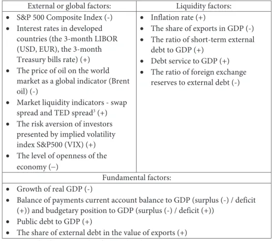
Following the earlier empirical analyses, we use explanatory variables in the model which are selected from the list shown in Table 1, while the expected sign of correlation of the specific variable with the dependent variable (EMBI spreads) is given in parentheses (see e.g., Prat, 2007).
Table 1. Possible explanatory variables
External or global factors: Liquidity factors: S&P 500 Composite Index (-)
Interest rates in developed countries (the 3-month LIBOR (USD, EUR), the 3-month Treasury bills rate) (+) The price of oil on the world
market as a global indicator (Brent oil) (-)
Market liquidity indicators - swap spread and TED spread3 (+)
The risk aversion of investors presented by implied volatility index S&P500 (VIX) (+) The level of openness of the
economy ()
Inflation rate (+)
The share of exports in GDP (-) The ratio of short-term external
debt to GDP (+)
Debt service to GDP (+) The ratio of foreign exchange
reserves to external debt (-)
Fundamental factors: Growth of real GDP (-)
Balance of payments current account balance to GDP (surplus (-) / deficit (+)) and budgetary position to GDP (surplus (-) / deficit (+))
Public debt to GDP (+)
The share of external debt in the value of exports (+)
Source: Authors’ presentation based on Prat (2007)
Disorders in broader market trends and the increasing risk aversion of investors cause a run in liquid assets and an increase in market yield spreads and interest rates (TED spread, swap spread, LIBOR). The increased probability of the country defaulting results in an increase in the EMBI spreads. The expected relationship between these external variables and the dependent variable is positive. It is important to note the impact of changes in the international risk-free interest rate, which is usually represented by the rate of return on U.S.
Treasury short-term government securities on the EMBI spreads. Given that the rate of return on a risky investment equals the risk-free interest rate plus a risk premium, the decline in the risk-free interest rate results in a decline in the rate of return on risky assets. The decline in global interest rates thus causes a decline in EMBI spreads. In addition, the decline in the international reference interest rate lowers liabilities based on variable debt and refinancing of debt, which has a positive effect on the solvency of developing countries. With lower risk of liquidity and solvency, debt appears sustainable, which, viewed from the perspective of market participants, lowers the probability of default and the yield spreads on debt securities of developing countries. Finally, the decline in international interest rates increases bond prices in developing countries due to the growth in demand for these yielding securities. This results in a drop in yield on risky securities and a narrowing of yield spreads. The high sensitivity of government bond yield spreads in developing countries compared to U.S. government bonds stems from the fact that these countries rely heavily on the U.S. dollar in foreign borrowing. Therefore, if interest rates rise in the country of the reserve currency, developing countries face an unfavourable debt position, especially if an increase in interest rates is accompanied by the appreciation of the dollar or other key reserve currency. In dual currency systems this problem is particularly acute. The growth in the value of the foreign currency in which the debt is denominated launches the spiral effect of ‘exchange rate - prices - exchange rate’, resulting in a further appreciation of foreign currency, with negative consequences for the country’s financial stability, budgetary position, and economic growth. This scenario has a significant additional impact on the yield spreads’ widening.
The solvency of a country indicates its ability to service its debts in the long run. Insolvency, as a result of inadequate structural parameters and the inherent economic weaknesses of a country, leads to difficulties in the fulfillment of the obligations that affect the perception of investors regarding the sustainability of, primarily, the country’s external debt.
default, and it is necessary to include this in a model that attempts to explain the behaviour of yield spreads in developing countries.
Finally, the level of the currency mismatch at the macro level will be presented by AECM and corrected AECM_COR measures, proposed by Goldstein and Turner (2004).
FC TD
XGS NFCA
AECM %
(2.6.)
If AECM 04
NFCA = NFAMABK + NBKA$ - NBKL$ - IB$ (2.7.)
DB IB DCP BKL NBKL
DB IB DCP BKL
NBKL TD
FC
$ $ $ $ $
% (2.8.)
Where:
NFCA = Net foreign currency assets,
FC%TD = Foreign currency share of domestic debt in the total debt, XGS = Exports of goods and services,
NFAMABK = Net foreign assets of monetary authorities and commercial banks, NBKA$ = Cross border assets in foreign currency of nonbanking sector at BIS reporting banks,
NBKL$ = Cross border liabilities in foreign currency of nonbanking sector to BIS reporting banks,
IB$ = International bonds outstanding in foreign currency,
NBKL = Cross border liabilities in all currencies of nonbanking sector to BIS reporting banks,
NBKL$ = Cross border liabilities in foreign currencies of nonbanking sector to BIS reporting banks,
BKL = Cross border liabilities in all currencies of banks to BIS reporting banks,
BKL$ = Cross border liabilities in foreign currencies of banks to BIS reporting banks,
DCP = Domestic loans to private sector,
DCP$ = Domestic loans to private sector in foreign currency, IB = International bonds outstanding in all currencies, DB = Domestic bonds outstanding in all currencies, DB$ = Domestic bonds outstanding in foreign currencies.
In basic calculations of the presented mismatch measure it is assumed that all domestic bonds and loans are denominated in local currency, i.e., DB$/DB=0 and DCP$/DCP=0.
The corrected measure AECM_COR takes into account the nonzero share of the domestic foreign currency debt in total, when these data are available for a particular country.
FC TD COR
XGS NFCA COR
AECM_ % _
(2.9.)
If AECM_COR 0
These measures show how vulnerable a country is in the case of significant depreciation of its currency. They take into account the currency composition of domestic and foreign assets and liabilities of different sectors of the economy. It is important to emphasize that the public sector, and the debt in foreign currency that it generates versus assets and income in local currency, is often the main generator of foreign exchange misbalances in developing countries. The indicators of aggregate currency mismatch show the net currency position of both debtor and creditor countries. If the level of negative currency mismatch of the debtor country is high, yield spreads on the debt of that country will grow, reflecting the increase in its probability of default. The reverse is the case with creditor countries, where the growth of positive currency misbalance leads to a decrease of yield spreads on its debt.
pre-emerging (frontier) markets5: Albania, Bulgaria, Montenegro, Croatia, FYR
Macedonia, Romania, Hungary, Czech Republic, Poland, Slovakia, Slovenia, Bosnia and Herzegovina, Estonia, Latvia, Lithuania, Serbia, Turkey, Ukraine, and Russia. Data were collected on solvency, liquidity, and external factors for the period 2001-2012. During the selection of explanatory variables, we rely on the previously mentioned studies that explain the behaviour of yield spreads on sovereign bonds. Then we introduce in the analysis the aggregate currency mismatch indicator in order to test its significance in the evaluation of the sensitivity of developing countries, which is reflected in the movement of their yield spreads on sovereign debt. A description of variables and data sources, together with the calculated aggregate currency mismatch indicator, is provided in the Appendix.
The analysis is performed on the sample of countries from Central and Eastern Europe and the Western Balkans for which we have the necessary data. From the sample of all countries for which there is available or we have calculated the aggregate indicators of currency mismatches (AECM and corrected measure AECM_COR), we will observe those for which we also have available market data of yield spreads on government debt securities (EMBI spreads). In the total period 2001-2012 the necessary data are available for five countries (Bulgaria, Hungary, Poland, Turkey and Russia). If we consider a shorter period, starting from 2005, the data are available for two additional countries, Serbia and Ukraine.
Initially, we observe data for five countries over a period of 12 years. Given that we have data for the explanatory and the dependent variables in every year, we have a balanced panel.
The basic model is first evaluated using a panel regression with fixed individual effects (FE model). In addition to the FE model we have also estimated the FE model with robust standard errors, which accounts for heteroskedasticity in
random errors. After testing and confirming the presence of heteroskedasticity and also the correlation of errors between the observation units in the same period of time, we have estimated specification by the Generalized Least Squares (GLS) method, which takes these facts into account.
In the second stage we have estimated a new model which includes the aggregate measure of currency mismatch and corrected aggregate currency mismatch as new explanatory variables, and we have tested their explanatory significance. The new model is also tested for the presence of heteroskedasticity in random errors and the correlation of errors between the observation units in the same period of time.
At this point it is important to note that the observed sample of countries is small for the implementation of dynamic panel model specifications and the observed time period is short for model estimation based on the e.g., Pooled Mean Group (PMG) estimation method.
The first step in the analysis6 is the presentation of summary descriptive
statistics of variables and detailed display of regressors’ variations within the observation units across time and between observation units (countries).7
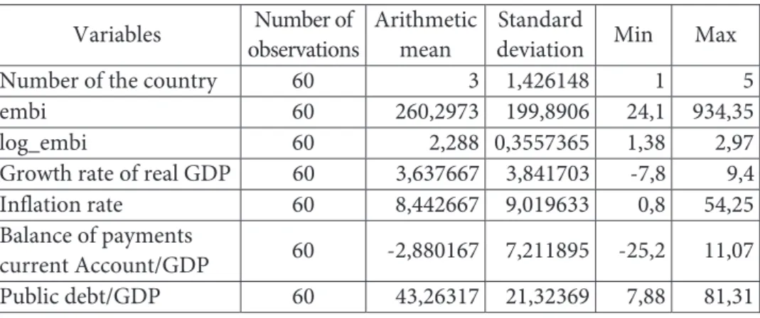
Table 2. Summary descriptive statistics of variables
Variables Number of observations
Arithmetic mean
Standard
deviation Min Max Number of the country 60 3 1,426148 1 5
embi 60 260,2973 199,8906 24,1 934,35
log_embi 60 2,288 0,3557365 1,38 2,97
Growth rate of real GDP 60 3,637667 3,841703 -7,8 9,4 Inflation rate 60 8,442667 9,019633 0,8 54,25 Balance of payments
current Account/GDP 60 -2,880167 7,211895 -25,2 11,07 Public debt/GDP 60 43,26317 21,32369 7,88 81,31
6 The analysis that follows was performed using the statistical/econometric software package Stata 11.
Fiscal position/GDP 60 -2,501 5,322289 -23,9 8,33 External debt/Exports 60 138,511 34,80216 85,32 226,23 Exports/GDP 60 45,1185 20,03306 21 94,66 Short-term external
debt/GDP 60 13,11983 8,525885 3,55 38,25 International
reserves/External debt 60 38,106 21,72739 15,71 99,06 External debt
service/GDP 60 10,0375 5,217186 3,25 22,43 3m LIBOR (usd) 60 2,264167 1,774974 0,34 5,3 3m LIBOR (eur) 60 2,515833 1,350998 0,57 4,63 3m-T-bill rate 60 1,783333 1,645056 0,05 4,73 Sp500_vix 60 21,86583 6,510219 12,81 32,69 Sp500 60 1186,159 157,6937 948,05 1477,18 Brent_oil 60 64,25917 30,58699 24,42 111,97
Aecm 60 -0,8283334 13,78823 -25 37,7
Aecm_cor 60 -3,73 18,91845 -45,5 38
EU member 60 0,3833333 0,4903014 0 1
Source: Authors' calculation
A detailed overview of descriptive statistics for EMBI spreads shows a slight asymmetry and a kurtosis slightly higher than normal.8 By taking the logarithm
of yield spreads, skewness and kurtosis decrease approaching the value characteristic for normal distribution. The significance (normality) test for coefficients of skewness and kurtosis shows that, for log-EMBI, variable asymmetry and kurtosis did not differ significantly from normal (p (skewness) = 0.1703, p (kurtosis) = 0.8766, adjusted χ2 (2) = 1.99, p> χ2 = 0.3702). By comparing the characteristics of these two variables we opt for log_EMBI as the dependent variable in the analysis, which is also the case in most of the related empirical analysis of yield spreads.
In the next step we examine the correlation between the dependent and all potential explanatory variables. We observe weak to moderate correlation
between different explanatory variables and between different variables and the log_EMBI variable.
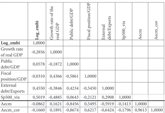
The selected explanatory variables and their correlation with the dependent variable and other explanatory variables are shown in Table 3.
Table 3. Correlation of variables
Log_embi Gro
w
th
r
at
e
o
f
th
e
re
al
G
D
P
Public
debt/GDP
Fiscal
position/GDP
External debt/Exports Sp500_v
ix
Aecm Aecm_
cor
Log_embi 1,0000
Growth rate
of real GDP -0,2856 1,0000
Public
debt/GDP 0,0578 -0,1872 1,0000
Fiscal
position/GDP -0,0310 0,4366 -0,5861 1,0000
External
debt/Exports 0,4550 -0,3846 0,4234 -0,5450 1,0000
Sp500_vix 0,5019 -0,4885 0,0643 -0,2121 0,2908 1,0000
Aecm -0,0862 0,1621 -0,8456 0,5495 -0,5919 -0,1413 1,0000
Aecm_cor -0,1660 0,1891 -0,8674 0,6217 -0,6424 -0,1796 0,9613 1,0000
Source: Authors’ calculation
It can be observed that AECM and especially AECM_COR measures are significantly correlated with the variable public debt/GDP, as well as moderately with fiscal position/GDP and external debt/exports, so it makes sense to replace these variables with aggregate measures of currency mismatch in subsequent model specifications. The significant correlation is due to the fact that the aggregate measure of currency mismatch implicitly reflects all the aforementioned macroeconomic imbalances in a single indicator.
and previous related empirical analysis. First, we model the behaviour of log_EMBI spreads by formulating a panel specification with fixed individual effects (and fixed effects with robust standard errors).9
The choice of a fixed model specification is primarily conditioned by the number of units of observation, i.e., the fact that we have restricted the conclusion-making to a specific set of several observation units (countries). This model is also verified on the basis of the Hausman specification test as the statistical criteria for choice. Besides the panel model with fixed effects, specification with random effects has also been tested on the same set of variables. The result of the Hausman test (χ2(4) statistic = 38.29, p = 0.0000) indicates the rejection of the null hypothesis where the model with random effects provides inconsistent estimates. So, between the two aforementioned specifications, we choose the specification with fixed effects, whose estimation by ordinary least squares (with fulfilled initial assumptions) provides us with consistent estimates of regression parameters. Fulfillment of these assumptions is further tested.
The test of individual effects confirms their significance (F(4.50) = 30.46, p > F = 0.0000). However, despite the significant individual effects, heteroskedasticity may be present in random errors and the possibility of disturbed assumption about the correlation of errors for different observation units in the same period of time.
In the next step we check whether there is a correlation of residuals between the observation units (countries) in the same period of time. The Breusch-Pagan LM test, for testing the presence of correlation between the residuals of observation units in the same period of time, is suitable for panels in which T is greater than N. According to this test, at the significance level of 5%, we reject
9 Regressors that were not statistically significant or that did not show the expected correlation
the null hypothesis according to which there is no statistically significant correlation between the residuals of different observation units (χ2(10) = 21.249, p = 0.0194).
We conclude that there exists a correlation between residuals of the different observation units, as a consequence of the common factors that influence all of the countries in the sample, or the fact that the counties are closely linked in economic terms.
Modified Wald's test was carried out for the presence of heteroskedasticity in the panel specification with fixed effects. It confirmed the presence of heteroskedasticity in the model (χ2(5) statistic = 58.69, p = 0.0000).
Because of the presence of correlation of residuals between the observation units as well as heteroskedasticity in the panel, we have tested the specification that takes into account these econometric problems. It is a fixed-effect specification estimated by the GLS method, in which we have additionally taken into account the correlation of residuals between the observation units and heteroskedasticity in the panel. A summary of different specifications estimated is given in Table 4.
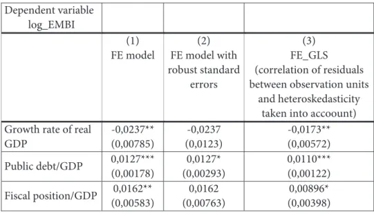
Table 4. Estimated panel specifications for the dependent variable log_EMBI on a sample of five countries in the period 2001-2012
Dependent variable log_EMBI
(1) FE model
(2) FE model with robust standard
errors
(3) FE_GLS
(correlation of residuals between observation units
and heteroskedasticity taken into accoount) Growth rate of real
GDP
-0,0237** (0,00785)
-0,0237 (0,0123)
-0,0173** (0,00572)
Public debt/GDP 0,0127*** (0,00178)
0,0127* (0,00293)
0,0110*** (0,00122)
Fiscal position/GDP 0,0162** (0,00583)
0,0162 (0,00763)
External debt/Exports
0,00230* (0,00111)
0,00230 (0,000927)
0,00263*** (0,000653)
Sp500_vix 0,0171*** (0,00369)
0,0171** (0,00348)
0,0164*** (0,00354)
bu -0,334***
(0,0359)
hu -0,991***
(0,0834)
po -0,726***
(0,0525)
tu -0,387***
(0,0720)
const 1,170*** (0,172)
1,170*** (0,136)
1,664*** (0,106)
N 60 60 60
r2 0,762 0,762
r2_o 0,151 0,151
r2_b 0,191 0,191
r2_w 0,762 0,762
sigma_u 0,395 0,395
sigma_e 0,156 0,156
rho 0,865 0,865
Source: Authors’ calculation
Notes:
1. Standard errors in parentheses 2. * p <0.05; ** p <0.01; *** p <0.001 3. Dummy variables:
bu (takes the value 1 for Bulgaria, and the value 0 for other countries) hu (takes the value 1 for Hungary, and the value 0 for other countries) po (takes the value 1 for Poland, and the value 0 for other countries) tu (takes the value 1 for Turkey, and the value 0 for other countries) ru (takes the value 1 for Russia, and the value 0 for other countries)
The first of the explanatory variables for the yield spreads’ behaviour is the analyzed countries’ real GDP growth rate. A higher level of economic growth lowers the debtor country’s probability of default, which is reflected in the reactions of market participants, who then require lower yields on the debt securities of the countries under consideration. Therefore, higher economic growth should lower yield spreads, which is confirmed by the negative sign of the estimated coefficient in front of this variable, observed in our sample of countries.
Coefficients in front of the variables public debt/GDP, fiscal position/GDP, and external debt/exports have the expected positive signs, indicating a positive relationship with yield spreads. The deterioration of the fiscal position of a country and an increase of its public and external debt increases the probability of a possible failure in the settlement of the country’s obligations, which is reflected in the growth of yield spreads on its debt securities.
The external global indicator of the increase in systemic risk, the implied volatility index SP500_vix, proved to be statistically significant. The growth of this indicator causes the growth of yield spreads as a response to an increase in systemic risk on a global level. This logic is confirmed by the estimated coefficient in front of the variable with a positive sign.
The specifications (2) and (3) have confirmed the findings of the FE model (1).
In the next step we want to test the significance of the aggregate currency mismatch variables, as more comprehensive indicators of the worsening of countries’ macroeconomic parameters that lead to the growth of risk and, in the extreme case, to default.
Specifications with fixed effects, fixed effects with robust standard errors, and a GLS specification that takes into account the confirmed correlation between the residuals of different observation units and heteroskedasticity in the panel are estimated.
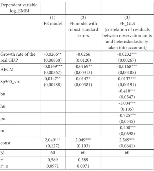
Table 5. Estimated panel specifications for the dependent variable log_EMBI with included measure of the aggregate currency mismatch (AECM) on a sample of five countries in the period 2001-2012
Dependent variable log_EMBI
(1) FE model
(2) FE model with robust standard
errors
(3) FE_GLS
(correlation of residuals between observation units
and heteroskedasticity taken into accoount) Growth rate of the
real GDP
-0,0266** (0,00830)
-0,0266 (0,0120)
-0,0232*** (0,00267)
AECM -0,0169*** (0,00367)
-0,0169** (0,00313)
-0,0168*** (0,00105)
Sp500_vix 0,0147** (0,00488)
0,0147* (0,00384)
0,0137*** (0,00191)
bu -0,418***
(0,0547)
hu -1,004***
(0,105)
po -0,725***
(0,0545)
tu -0,400***
(0,0698)
const 2,049*** (0,127)
2,049*** (0,103)
2,569*** (0,0641)
N 60 60 60
r2 0,589 0,589
r2_b 0,147 0,147
r2_w 0,589 0,589
sigma_u 0,383 0,383
sigma_e 0,201 0,201
rho 0,784 0,784
Source: Authors’ calculation
Notes:
1. Standard errors in parentheses 2. * p <0.05; ** p <0.01; *** p <0.001 3. Dummy variables:
bu (takes the value 1 for Bulgaria, and the value 0 for other countries) hu (takes the value 1 for Hungary, and the value 0 for other countries) po (takes the value 1 for Poland, and the value 0 for other countries) tu (takes the value 1 for Turkey, and the value 0 for other countries) ru (takes the value 1 for Russia, and the value 0 for other countries)
The analysis was also undertaken with the corrected measure of aggregate currency mismatch (AECM_COR) included, which more informatively demonstrates the level of currency misbalances in specific markets. The main findings do not differ from the previous ones.10
On the basis of estimated specifications on a sample of five countries from Central and Eastern Europe and the Western Balkans we can conclude the following:
The measures of indebtedness and fiscal position of the countries included in the specifications influence the behaviour of government debt security yield spreads, in relation to the representative securities of developed countries. The signs in front of the estimated coefficients of the observed explanatory
variables follow economic logic. The worsening of the budgetary position of the country, the increase of its public and external debt, increases the probability of the country defaulting or being unable to meet its obligations. When these obligations are denominated in foreign currency, which is also the specificity of dual currency systems, it is impossible to ignore the connection between the increase in demand for foreign currency, the
through of that effect on prices, rising inflationary pressures that continue to increase demand for foreign currency, and negative repercussions for local financial stability and economic growth. The negative consequences for economic growth further increase the risk of the country’s default and yield spreads are being perceived as indicators of that probability by market transactors.
The worsening of external macro factors, in this context presented by S&P500 volatility index VIX, leads to an increase in yield spreads as indicators of default risk.
By substituting indicators of the fiscal position and indebtedness with the aggregate and the corrected aggregate measure of currency mismatch, the explanatory power of these aggregate indicators for the behaviour of yields on government debt securities has been confirmed. The new model also confirms the robustness of the basic model. The increase of negative currency mismatch leads to the growth of macro risks, reflected in the increase of yield spreads on government securities.
Due to the fact that all estimated specifications are in log-linear form, estimated coefficients are interpreted as follows: the slope coefficients in front of the regressor indicate the relative (%) change in the dependent variable Y with respect to the absolute change in explanatory variable X; i.e., with growth of X for one unit, Y is changed on average by 100%*β.
The presented analysis was also repeated on the broader sample of seven countries’ (Bulgaria, Hungary, Poland, Serbia, Russia, Turkey, Ukraine) data for
the period 2005-2012.11
The conclusions based on a sample of seven countries do not differ substantially from the conclusions of the previous analysis on a sample of five countries, representing a specific robustness check for the estimated models. The estimated coefficients in front of the aggregate indicators of currency mismatch confirm the significance of these measures in explaining the behaviour of yield spreads as indicators of the analyzed countries’ default risk.
4. CONCLUSION
The presented analysis on samples of five and seven developing countries from the regions of Central and Eastern Europe and the Western Balkans is, to the authors' knowledge, so far unique for this region, and thus is potentially very significant. It is important to point out that the authors have, for the first time, calculated the aggregate indicators of currency mismatch for nine additional countries, in comparison to the existing base of BIS.
The aim of the empirical analysis was to demonstrate, taking into account the standard explanatory factors for the behaviour of yield spreads on government securities, that the additional indicators of financial fragility are essential when analyzing the sensitivity of developing countries to depreciation of local currencies. The analysis of yield spreads through panel models allowed comparison of the results of specifications that have taken into account the relevant fundamental and external explanatory factors for the movement of spreads with specifications that include aggregate measures of currency mismatch.
The analysis shows that aggregate currency mismatch and corrected aggregate currency mismatch measures are important and useful indicators that show in a comprehensive way the effect of important macroeconomic variables that may be the cause of both stability and significant disturbances at the macro level of a country. In this case, in the analyzed samples of developing countries, currency mismatch measures have been observed instead of individual indicators of budgetary position and indebtedness. It turned out that mismatch indicators are negatively correlated with yield spreads, confirming the logic that a higher level of debt, especially when the debt is in foreign currency while the country generates revenues in local currency, leads to an increase in the probability of default, and the increase in yield spreads indicates that probability.
depreciation impact. The currency crises in these countries are usually followed by crises in the banking sector and/or balance of payment crises. These aspects of the problem represent fruitful areas for further research.
Due to the significance of the analyzed problem, policy makers in developing countries, including Serbia, should regularly calculate and publish the level of currency mismatch, as one of the initial steps in the fight against currency misbalance at the macro level and the level of all relevant sectors of the economy.
REFERENCES
Aghion, P., Bacchetta, P. & Banerjee, A. (2001). Currency Crises and Monetary Policy in an Economy with Credit Constraints. European Economic Review, 45 (7), pp. 1121-1150.
Aghion, P., Bacchetta, P. & Banerjee, A. (2004). A Corporate Balance-Sheet Approach to Currency Crises. Journal of Economic heory, 119 (1), pp. 6-30.
Akitoby, B. & Stratmann, T. (2008). Fiscal Policy and Financial Markets. he Economic Journal, 118 (November), pp. 1971–1985.
Arora V. & Cerisola, M. (2001). How Does U.S. Monetary Policy Inluence Sovereign Spreads in Emerging Markets? (IMF Staf Papers, Vol. 48, No. 3), Washington, D.C.: International Monetary Fund
Baldacci, E., Gupta, S. & Mati, A. (2008). Is it (Still) Mostly Fiscal? Determinants of Sovereign Spreads in Emerging Markets (IMF Working Paper WP/08/259), Washington D.C.: International Monetary Fund
Bellas, D., Papaioannou, M. G. & Petrova, I. (2010). Determinants of Emerging Market Sovereign Bond Spreads: Fundamentals vs Financial Stress (IMF Working Paper WP/10/281), Washington D.C.: International Monetary Fund
Božović, M., Urošević, B. & Živković, B. (2009). On the Spillover of Exchange Rate Risk into Default Risk. Economic Annals, 183, pp. 32–55.
Buckley, R. P. & Dirou, P. (2006). How to Strengthen the International Financial System by Restructuring Sovereign Balance Sheets. Annals of Economics and Finance, 2, pp. 257-269. Céspedes, L., Chang, R. & Velasco, A. (2000). Balance Sheets and Exchange Rate Policy (NBER Working Paper 7840), Cambridge, MA: National Bureau of Economic Research
Céspedes, L., Chang, R.& Velasco, A. (2004). Balance Sheets and Exchange Rate Policy. he American Economic Review, 94 (4), pp. 1183-1193.
Dailami, M., Masson, P. R. & Padou, J. J. (2005). Global Monetary Conditions versus Country-Speciic Factors in the Determination of Emerging Market Spreads. International Finance 0506003, EconWPA
Diamond, D. W. (1989). Reputation Acquisition in Debt Markets. Journal of Political Economy, 97 (4), pp. 828-862.
Dornbusch, R. (2001). A Primer on Emerging Market Crises (NBER Working Paper 8326), Cambridge, MA: National Bureau of Economic Research
Edwards, S. (1986). he Pricing of Bonds and Bank Loans in International Markets: An Empirical Analysis of Developing Countries’ Foreign Borrowing. European Economic Review, 30(3), pp. 565–589.
Eichengreen B. & Mody, A. (1998). What Explains Changing Spreads on Emerging Market Debt: Fundamentals or Market Sentiment? (NBER Working Paper 6408), Cambridge, MA: National Bureau of Economic Research
Ferrucci, G. (2003). Empirical Determinants of Emerging Market Economies’ Sovereign Bond Spreads (Bank of England Working Paper 205)
Goldstein, M. & Turner, P. (2004). Controlling Currency Mismatches In Emerging Markets. Washington, D. C.: Institute for International Economics.
Hartelius, K., Kashiwase, K. & Kodres, L. E. (2008). Emerging Market Spread Compression: Is it Real or is it Liquidity? (IMF Working Paper WP/08/10), Washington D.C.: International Monetary Fund
Hilscher, J., & Nosbusch, Y. (2009). Determinants of Sovereign Risk: Macroeconomic Fundamentals and the Pricing of Sovereign Debt. Retrieved from http://personal.lse.ac.uk/ nosbusch/hilschernosbusch.pdf
Kamin, S.B. & Von Kleist, K. (1999). he Evolution and Determinants of Emerging Market Credit Spreads in the 1990s (International Finance Discussion Papers, 653), Board of Governors of the Federal Reserve System
Krugman, P. (1999). Balance Sheets, the Transfer Problem, and Financial Crises. In P. Isard, A. Razin, and A. K. Rose (Eds.), International Finance and Financial Crises. Kluwer Academic Publishers and IMF
McGuire, P. & Schrijvers, M. A. (2003). Common Factors in Emerging Market Spreads (BIS Quarterly Review, December), Basel: Bank for International Settlements
Prat, S. 2007. he Relevance of Currency Mismatch Indicators: an Analysis through Determinants of Emerging Market Spreads. Economie Internationale, 111 (3), pp. 101-122.
Rosenberg, C., Halikias, I., House, B., Keller, C., Nystedt, J., Pitt, A. & Setser, B. (2004). Debt-Related Vulnerabilities and Financial Crises - An Application of the Balance Sheet Approach to Emerging Market Countries (IMF Policy Development and Review Department Paper), Washington D.C.: International Monetary Fund
Rowland, P. (2004). Determinants of Spread and Creditworthiness for Emerging Market Sovereign Debt: A Follow-Up Study Using Pooled Data Analysis. Borradores de Economia 296, Banco de la Republica de Colombia
Rowland, P. & Torres, J. L. (2004). Determinants of Spread and Creditworthiness for Emerging Market Sovereign Debt: A Panel Data Study. Borradores de Economia 295, Banco de la Republica de Colombia
APPENDIX
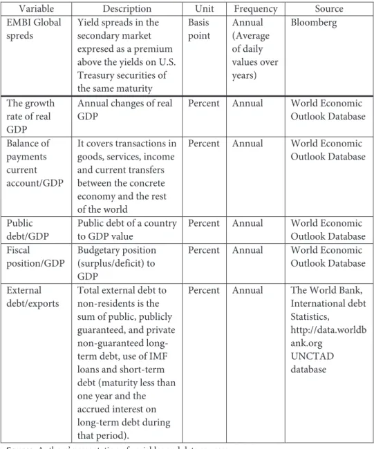
Table A.1. Description of variables and data sources - dependent variable and fundamental factors
Variable Description Unit Frequency Source
EMBI Global spreds
Yield spreads in the secondary market expresed as a premium above the yields on U.S. Treasury securities of the same maturity
Basis point Annual (Average of daily values over years) Bloomberg The growth rate of real GDP
Annual changes of real GDP
Percent Annual World Economic
Outlook Database
Balance of payments current account/GDP
It covers transactions in goods, services, income and current transfers between the concrete economy and the rest of the world
Percent Annual World Economic
Outlook Database
Public debt/GDP
Public debt of a country to GDP value
Percent Annual World Economic
Outlook Database Fiscal position/GDP Budgetary position (surplus/deficit) to GDP
Percent Annual World Economic
Outlook Database
External debt/exports
Total external debt to non-residents is the sum of public, publicly guaranteed, and private non-guaranteed long-term debt, use of IMF loans and short-term debt (maturity less than one year and the accrued interest on long-term debt during that period).
Percent Annual The World Bank,
International debt Statistics, http://data.worldb ank.org UNCTAD database
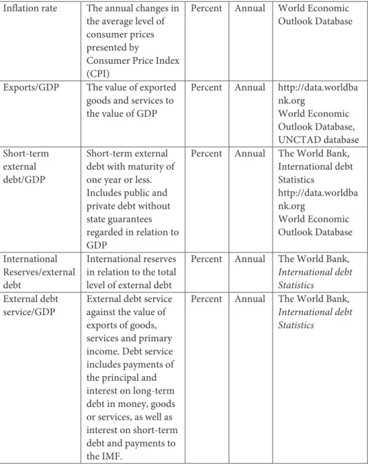
Table A.2. Description of variables and data sources - indicators of liquidity
Inflation rate The annual changes in the average level of consumer prices presented by
Consumer Price Index (CPI)
Percent Annual World Economic
Outlook Database
Exports/GDP The value of exported goods and services to the value of GDP
Percent Annual http://data.worldba nk.org World Economic Outlook Database, UNCTAD database Short-term external debt/GDP Short-term external debt with maturity of one year or less. Includes public and private debt without state guarantees regarded in relation to GDP
Percent Annual The World Bank, International debt Statistics http://data.worldba nk.org World Economic Outlook Database International Reserves/external debt International reserves in relation to the total level of external debt
Percent Annual The World Bank,
International debt Statistics
External debt service/GDP
External debt service against the value of exports of goods, services and primary income. Debt service includes payments of the principal and interest on long-term debt in money, goods or services, as well as interest on short-term debt and payments to the IMF.
Percent Annual The World Bank,
International debt Statistics
Table A.3. Description of variables and data sources - external factors
3m-LIBOR (usd)
The interest rate at which banks offer each other money for borrowing in the London interbank market. Percent Annual rate Eurostat 3m-T-bill rate
The rate of return on three-month US Treasury bills. Percent Annual rate http://www.treas ury.gov
VIX Volatility index Index
points
Annual averages
CBOE
S&P500 Index that tracks the movement of the market value of 500 actively traded stocks of the most valuable companies in the U.S. market
Index points Annual averages NYSE Brent oil prices on the world market
USD Annual Bloomberg
Source: Authors’ presentation of variables and data sources
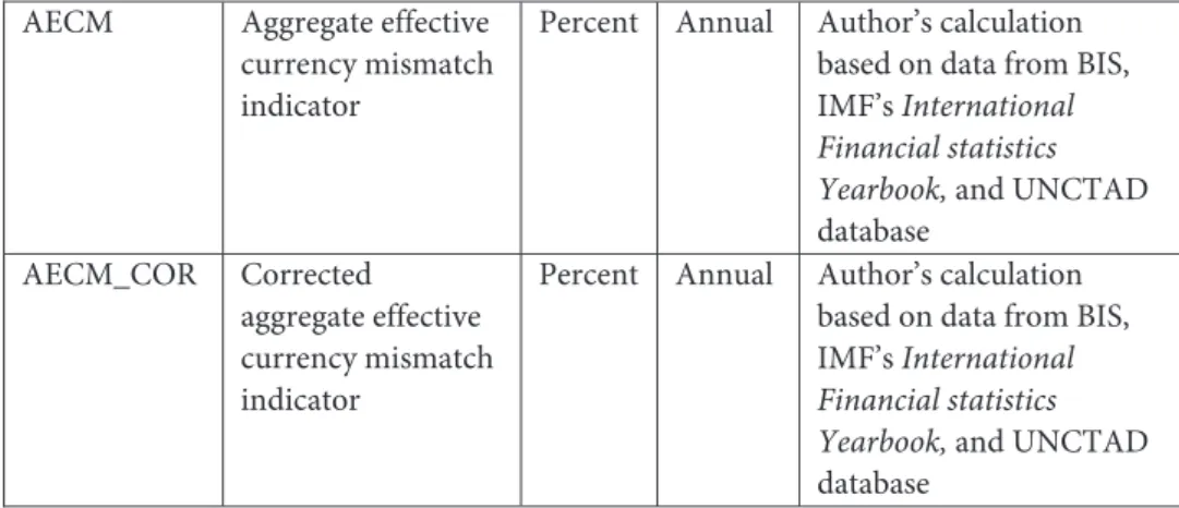
Table A.4. Description of variables and data sources - indicators of aggregate currency mismatch
AECM Aggregate effective
currency mismatch indicator
Percent Annual Author’s calculation based on data from BIS, IMF’s International Financial statistics Yearbook, and UNCTAD database
AECM_COR Corrected aggregate effective currency mismatch indicator
Percent Annual Author’s calculation based on data from BIS, IMF’s International Financial statistics Yearbook, and UNCTAD database
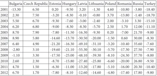
Table A.5. Aggregate measure of currency mismatch for 10 countries in Central and Eastern Europe in the BIS database (AECM), in %
Bulgaria Czech Republic Estonia Hungary Latvia Lithuania Poland Romania Russia Turkey
2001 -13.30 6.50 0.20 -9.50 3.20 -1.30 4.60 -10.80 -3.80 -18.40
2002 2.30 7.50 -3.20 -8.30 -0.10 -0.80 3.70 -13.80 -1.40 -18.70
2003 5.50 6.70 -9.30 -7.60 -3.00 -2.40 2.00 -3.10 3.30 -15.10
2004 6.20 6.80 -9.00 -8.30 -8.30 -5.70 2.50 1.70 12.00 -11.10
2005 8.70 7.90 -7.80 -11.50 -16.30 -9.30 0.20 -7.00 21.70 -9.00
2006 8.90 5.80 -14.60 -13.70 -30.50 -20.00 -1.50 0.60 30.00 -8.30
2007 6.40 4.90 -21.20 -16.30 -49.10 -31.10 -3.20 -10.40 35.60 -7.60
2008 -2.80 3.10 -19.60 -21.10 -55.30 -30.10 -5.70 -17.30 27.50 -7.90
2009 -1.10 3.30 -17.50 -25.00 -48.10 -39.30 -8.10 -24.30 37.70 -8.00
2010 2.60 2.30 -8.70 -15.80 -27.40 -25.80 -6.60 -20.00 26.80 -9.50
2011 4.70 1.50 -6.30 -11.00 -13.20 -17.80 -5.10 -16.00 20.30 -10.40
2012 6.70 1.70 -7.80 -8.10 -12.60 -14.60 -4.80 -17.40 17.80 -9.80
Source: BIS
Note: AECM = (NFCA/XGS)*FC%TD if AECM<0 and AECM = (NFCA/MGS)* FC%TD if
AECM>0; assuming that the share of domestic debt in foreign currency is equal to 0.
Table A.6. Corrected aggregate measure of currency mismatch for 10 countries in Central and Eastern Europe in the BIS database (AECM_COR), in %
Bulgaria Czech Republic Estonia Hungary Latvia Lithuania Poland Romania Russia Turkey
2001 -13.30 10.00 0.20 -13.80 4.00 -2.20 10.90 -10.80 -3.80 -42.00
2002 2.60 10.80 -3.20 -12.90 -0.10 -1.30 8.10 -13.80 -1.40 -45.50
2003 8.20 9.50 -20.60 -11.80 -6.90 -3.80 3.70 -3.10 3.40 -32.10
2004 10.30 9.10 -16.90 -13.40 -19.20 -9.50 4.10 1.70 12.70 -20.90
2005 16.70 10.00 -14.80 -18.10 -36.00 -17.20 0.30 -7.00 22.60 -14.60
2006 14.90 7.40 -29.80 -21.30 -66.20 -30.80 -2.30 0.60 30.90 -11.90
2007 11.10 6.00 -43.10 -27.20 -104.70 -48.60 -5.00 -10.40 36.20 -10.40
2008 -4.90 3.90 -40.70 -34.90 -113.70 -50.90 -9.90 -17.30 27.70 -10.50
2009 -2.00 4.20 -40.50 -40.30 -101.10 -67.40 -13.60 -24.30 38.00 -11.50
2010 5.40 2.90 -22.20 -27.00 -60.80 -44.70 -11.10 -20.00 27.10 -15.50
2011 11.40 1.90 -6.50 -18.40 -32.60 -30.80 -8.70 -16.00 20.30 -17.00
2012 16.40 2.10 -8.30 -13.70 -27.00 -25.40 -8.00 -17.40 17.80 -15.90
Source: BIS
Note: AECM_COR = (NFCA/XGS)*FC%TD_COR if AECM_COR<0 and AECM_COR =
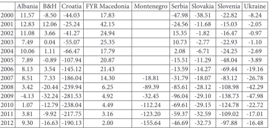
Table A.7. Aggregate measure of currency mismatch for 9 additional countries in Central and Eastern Europe and Western Balkans (AECM), in %
Albania B&H Croatia FYR Macedonia Montenegro Serbia Slovakia Slovenia Ukraine
2000 11.57 -8.50 -44.03 17.83 -47.98 -38.51 -22.82 -8.24
2001 12.83 12.06 -25.24 42.15 -24.56 -11.68 -15.03 -2.05
2002 11.08 3.66 -41.27 24.94 15.35 -1.82 -16.47 -0.97
2003 7.49 0.04 -55.07 25.35 10.73 -2.77 -22.93 -1.10
2004 10.06 1.11 -66.47 17.79 2.08 -6.71 -24.25 -2.69
2005 7.89 -0.89 -107.94 20.87 -15.51 -11.29 -48.04 -3.89
2006 8.13 3.54 -145.12 21.43 -13.59 -14.27 -69.44 -19.16
2007 8.51 7.33 -186.04 14.30 -18.81 -31.79 -18.07 -83.12 -26.78
2008 3.42 -20.44 -239.94 6.25 -89.39 -85.61 -28.12 -108.98 -42.29
2009 -4.13 -32.24 -281.53 4.92 -32.45 -96.04 -29.10 -138.73 -47.98
2010 1.07 -12.79 -238.04 4.49 -112.24 -69.61 -29.15 -124.78 -22.72
2011 3.81 -9.92 -217.75 3.16 -123.20 -59.37 -32.59 -109.02 -17.01
2012 9.30 -16.63 -190.13 2.00 -155.64 -46.69 -32.73 -97.88 -16.48
Source: Authors’ calculation based on the BIS, IMF, WB, UNCTAD data and national sources
Note: AECM = (NFCA/XGS)*FC%TD if AECM<0 and AECM = (NFCA/MGS)*FC%TD if
AECM>0; assuming that the share of domestic debt in foreign currency is equal to 0.
Table A.8. Corrected aggregate measure of currency mismatch for 9 additional countries in Central and Eastern Europe and Western Balkans (AECM_COR), in %
Albania B&H Croatia Macedonia Montenegro Serbia Slovakia Slovenia Ukraine
2000 11.57 -8.50 -44.03 17.83 -88.01 -38.51 -22.82 -8.24
2001 12.83 12.06 -25.24 42.15 -62.60 -11.68 -15.03 -2.05
2002 11.08 3.66 -41.27 24.94 33.98 -1.82 -16.47 -0.97
2003 7.49 0.04 -55.07 25.35 25.39 -2.77 -22.93 -1.10
2004 10.06 1.11 -66.47 17.79 3.75 -6.71 -24.25 -2.69
2005 7.89 -0.89 -107.94 20.87 -21.79 -11.29 -48.04 -3.89
2006 8.13 3.54 -145.12 21.43 -17.12 -14.27 -69.44 -19.16
2007 8.51 7.33 -186.04 14.30 -18.81 -41.55 -18.07 -83.12 -26.78
2008 3.42 -20.44 -239.94 6.25 -89.39 -107.52 -28.12 -108.98 -42.29
2009 -4.13 -32.24 -281.53 4.92 -32.45 -124.10 -29.10 -138.73 -47.98
2010 1.07 -12.79 -238.04 4.49 -112.24 -93.63 -29.15 -124.78 -22.72
2011 3.81 -9.92 -217.75 3.16 -123.20 -78.30 -32.59 -109.02 -17.01
2012 9.30 -16.63 -190.13 2.00 -155.64 -65.72 -32.73 -97.88 -16.48
Source: Authors’ calculation based on the BIS, IMF, WB, UNCTAD data and national sources
Note: AECM_COR = (NFCA/XGS)*FC%TD_COR if AECM_COR<0 and AECM_COR =
Figure A.1. EMBI spreads for selected countries of Central and Eastern Europe and the Western Balkans
Source: Authors’ presentation based on Bloomberg’s data
Table A.9. Detailed presentation of variations of the regressors over time within and between units of observation (country)
Variable
Mean Stanard
deviation
Min. Max.
Observations
Country number Overall 3 1.426148 1 5 N = 60
Between 1.581139 1 5 n = 5
Within 0 3 3 T = 12
embi Overall 260.2973 199.8906 24.1 934.35 N = 60
Between 108.825 139.9042 404.145 n = 5
Within 174.1303 42.32066 865.6106 T = 12
log_embi Overall 2.288 0.3557365 1.38 2.97 N = 60
Between 0.2213034 2.043333 2.555 n = 5
Within 0.2944558 1.624667 2.934667 T = 12
Growth rate of the real GDP
Overall 3.637667 3.841703 -7.8 9.4 N = 60
Between 1.175457 1.683333 4.755 n = 5
Inflation rate
Overall 8.442667 9.019633 0.8 54.25 N = 60
Between 5.606137 2.969167 16.6925 n = 5
Within 7.468909 -1.999833 46.00017 T = 12
Balance of payments current account/GDP
Overall -2.880167 7.211895 -25.2 11.07 N = 60
Between 6.12126 -8.868333 7.49 n = 5
Within 4.639775 -19.21183 6.928167 T = 12
Public debt/GDP
Overall 43.26317 21.32369 7.88 81.31 N = 60
Between 19.07365 18.86917 67.43833 n = 5
Within 12.59856 28.2315 81.8715 T = 12
Fiscal position/GDP
Overall -2.501 5.322289 -23.9 8.33 N = 60
Between 3.700124 -5.5325 2.555833 n = 5
Within 4.145888 -20.8685 6.660667 T = 12
External
debt/Exports Overall 138.511 34.80216 85.32 226.23 N = 60
Between 27.60359 103.0592 180.1133 n = 5
Within 24.3165 93.84767 225.1268 T = 12
Exports/GDP Overall 45.1185 20.03306 21 94.66 N = 60
Between 20.86138 23.705 76.47167 n = 5
Within 6.874923 29.64683 63.30684 T = 12
Short-term external debt/GDP
Overall 13.11983 8.525885 3.55 38.25 N = 60
Between 7.222114 4.846667 23.00333 n = 5
Within 5.500576 -1.0935 28.3665 T = 12
International reserves/External debt
Overall 38.106 21.72739 15.71 99.06 N = 60
Between 19.60705 23.23583 71.27833 n = 5
Within 12.62211 -10.11233 65.88766 T = 12
External debt service/GDP
Overall 10.0375 5.217186 3.25 22.43 N = 60
Between 3.99239 4.273333 13.80583 n = 5
Within 3.775124 3.111667 18.67917 T = 12
3m LIBOR (usd)
Between 0 2.264167 2.264167 n = 5
Within 1.774974 0.34 5.3 T = 12
3m LIBOR (eur)
Overall 2.515833 1.350998 0.57 4.63 N = 60
Between 0 2.515833 2.515833 n = 5
Within 1.350998 0.57 4.63 T = 12
3m-T-bill rate
Overall 1.783333 1.645056 0.05 4.73 N = 60
Between 0 1.783333 1.783333 n = 5
Within 1.645056 0.05 4.73 T = 12
Sp500_vix Overall 21.86583 6.510219 12.81 32.69 N = 60
Between 0 21.86583 21.86583 n = 5
Within 6.510219 12.81 32.69 T = 12
Sp500 Overall 1186.159 157.6937 948.05 1477.18 N = 60
Between 0 1186.159 1186.159 n = 5
Within 157.6937 948.05 1477.18 T = 12
Brent_oil
Overall 64.25917 30.58699 24.42 111.97 N = 60
Between 0 64.25917 64.25917 n = 5
Within 30.58699 24.42 111.97 T = 12
Aecm Overall -0.8283334 13.78823 -25 37.7 N = 60
Between 12.85997 -13.01667 18.95833 n = 5
Within 7.45452 -23.58667 17.91333 T = 12
Aecm_cor Overall -3.73 18.91845 -45.5 38 N = 60
Between 17.46913 -21.06667 19.29167 n = 5
Within 10.47061 -28.58 14.97833 T = 12
t Overall 6.5 3.481184 1 12 N = 60
Between 0 6.5 6.5 n = 5
Within 3.481184 1 12 T = 12
EU member Overall 0.3833333 0.4903014 0 1 N = 60
Between 0.3754627 0 0.75 n = 5
Within 0.3545507 -0.3666667 0.9666667 T = 12
Table A.10. Descriptive statistics for variables EMBI and log_EMBI
embi Log_embi
N 60 60
Arithmetic mean 260,2973 2,288
Standard deviation 199,8906 0,3557365
Skewness coefficient 1,541122 -0,4055467
Kurtosis coefficient 5,490419 2,72407
Source: Authors’ calculation