Escola de Pós-Graduação em Economia - EPGE
Fundação Getulio Vargas
The Asymmetric Behavior of the
U.S. Public Debt
Dissertação submetida à Escola de Pós-Graduação em Economia da Fundação Getulio Vargas como requisito para obtenção do
Título de Mestre em Economia
Aluna: Raquel Menezes Bezerra Sampaio
Orientador: Luiz Renato Lima
Escola de Pós-Graduação em Economia - EPGE
Fundação Getulio Vargas
The Asymmetric Behavior of
the U.S. Public Debt
Dissertação submetida à Escola de Pós-Graduação em Economia da Fundação Getulio Vargas como requisito para obtenção do
Título de Mestre em Economia
Aluna: Raquel Menezes Bezerra Sampaio
Banca Examinadora:
Luiz Renato Lima (Orientador, EPGE/FGV) João Vítor Issler (EPGE/FGV)
Fabiana Fontes Rocha (FEA/USP)
Abstract
1
Introduction
For decades, a lot of e¤ort has been devoted to investigate whether long-lasting budget de…cits represent a threat to public debt sustainability. Hamilton and Flavin (1986) was one of the …rst studies to address this question testing for the non-existence of ponzi scheme in public debt. They conducted a battery of tests using data from the period 1962-84 and assuming a …xed interest rate. Their results indicate that the government intertemporal budget constraint holds. In a posterior work, Wilcox (1989) extends Hamilton and Flavin’s work by allowing for stochastic variation in the real interest rate. His focus was on testing for the validity of the present-value borrowing constraint, which means that the public debt will be sustainable in a dynamically e¢cient economy1 if the
discounted public debt is stationary with unconditional mean equal to zero.
An important and common feature in the aforementioned studies is the underlying assumption that economic time series possess symmetric dynamics. In recent years, considerable research e¤ort has been devoted to study the e¤ect of di¤erent …scal regimes on long-run sustainability of the public debt. For instance, Davig (2004) uses a Markov-switching time series model to analyze the behavior of the discounted U.S. Federal debt. The author uses an extended version of Hamilton and Flavin (1986) and Wilcox (1989) data and identi…es two …scal regimes: in the …rst one the discounted Federal debt is expanding whereas it is collapsing in the second one. He concludes that although the expanding regime is not sustainable, it does not pose a threat to the long run sustainability of the discounted U.S. federal debt. Arestis et al. (2004) model the U. S. government de…cit per capita using a threshold autoregressive model. Two …scal policy regimes are identi…ed by the extent of the semi-annual change in the de…cit. Using quarterly de…cit data from the period 1947:2 to 2002:1, they …nd evidence that the U.S. budget de…cit is sustainable in the long run and that economic policy makers only intervene to reduce budget de…cit when it reaches a certain threshold, deemed to be unsustainable.
In this paper we reanalyze the question of public debt sustainability using the quantile autore-gression model recently developed by Koenker and Xiao (2004a). In this new model, the autoregress-ive coe¢cient may take di¤erent values (possibly unity) over di¤erent quantiles of the innovation process. Some forms of the quantile autoregressive (QAR) model can exhibit unit-root like beha-vior, but with occasional episodes of mean reversion su¢cient to insure stationarity. We use an extension of Hamilton and Flavin (1986) and Wilcox (1989) data, provided by Davig (2004). As in Wilcox (1989), our data set allows for stochastic interest rate as we deal with the discounted public debt series. We believe that this modelling is ideal for the following reasons:
dynamic;
- it is possible to test for both global and local sustainability. The latter allows us to identify …scal policies (trajectories of public debt) that are not consistent with public debt sustainability in the sense that if they were allowed to persist inde…nitely, would eventually violate intertemporal restrictions;
- in contrast to the threshold autoregressive model used by Arestis et al. (2004), we do not have to consider only two regimes and split the sample points into them. This avoids identi…cation problems in short samples;
- unlike Davig (2004) that assumes an autoregressive process with just one lag and a determ-inistic …rst-order autoregressive coe¢cient, we consider the possibility that the discounted U.S. Federal debt series can be represented by a autoregressive process with p lags,p 1, in which all autoregressive coe¢cients are random. In the Davig (2004) approach, only the intercept is allowed to change across regimes and the process is assumed to be local as well as globally stationary. Consequently, the author does not test for local and global stationarity. Thus, the tests for local and global public debt sustainability in Davig (2004) consist in verifying if the unconditional mean of the debt process is not signi…cantly di¤erent from zero. In this paper, we will investigate if both conditions (stationarity and zero unconditional mean) holds locally as well as globally;
- it permits to identify the dynamic of the discounted U.S. Federal debt at di¤erent quantiles. Hence, we can easily forecast debt values that should be avoided by policy makers if they were interested in keeping public debt sustainable. We believe that policy makers might be interested in using such forecasts as guidance instruments for monetary and …scal policies;
- in contrast to both Davig (2004) and Arestis et al. (2004), our estimation procedure does not require a distribution speci…cation for the innovation process, which makes our approach robust against distribution misspeci…cation. Indeed, estimation in Davig (2004) and Arestis et al. (2004) are based on maximum likelihood2, which requires distribution speci…cation. Quantile regression method is robust to distributional assumptions, a property that is inherited from the robustness of the ordinary sample quantiles. Moreover, in quantile regression, it is not the magnitude of the dependent variable that matters but its position relative to the estimated hyperplane. As a result, the estimated coe¢cients are not sensitive to outlier observations. Such property is especially attractive in our application since public debt may be contaminated by outlier observations coming from periods of war, oil shocks and political turmoil.
Our results expand previous …ndings on public debt sustainability reported in the literature. Unlike Davig (2004), the quantile estimates provide evidence of what we have called band of
tainability: the discounted U.S. federal debt is sustainable for values inside the band, but becomes unsustainable when it jumps out of the band. In other words, the …scal policy follows three di¤erent dynamics according to the level of the discounted U.S. Federal debt: (1) for values around (and inclusive) the median, …scal policy is sustainable, ruling out the possibility of permanent budget de…cits; (2) when public debt attains high values (high quantiles), …scal policy turns out to be unsustainable, with the discounted debt not converging to zero, even though it follows a stationary path; (3) when the debt is low (low quantiles), …scal policy is unsustainable, presenting both non-stationarity and non-zero (and negative) unconditional mean. Despite the occasional episodes in which the discounted U.S. federal debt moves out of the band of sustainability, our results indicate that the U.S. debt is globally sustainable, i.e., the periods in which public debt is too high or too low do not seem to persist forever. This suggests that the U.S. government has been committed with long-run sustainability of the public debt, bringing it back to its sustainability band whenever it moves out.
2
Theory: the present-value borrowing constraint
The accumulation of government debt follows the equation:
bt= (1 +rt 1)bt 1 st (1)
where:
bt is the market value of the government debt in constant dollars;
rt 1 is the ex-post real interest rate
st is the noninterest surplus in constant dollars.
Letqt be the real discount factor from period t back to period zero, de…ned by:
qt= t 1
Y
j=0
1 (1 +rj)
; t= 1;2; ::
and q0= 1
thus, qt is a function of (r0;r1;:::; rt 1) and it is known at period t.
Usingqt it is possible to rewrite equation (1) with each variable discounted to period zero:
qtbt = qt(1 +rt 1)bt 1 qtst
qtbt = qt 1bt 1 qtst
Let Bt := qtbt be the discounted value of debt in period t back to period zero, and St := qtst be the discounted value of the surplus in period t back to period zero. Then:
Bt=Bt 1 St:
Solving equation by recursive forward substitution leads to:
Bt=Bt+N+ N
X
j=1
St+j: (2)
of the debt is expected to be equal to the discounted value of the sum of all future noninterest surpluses:
Bt= lim
N!1EtBt+N+ 1
X
j=1
EtSt+j
lim
N!1EtBt+N = 0)
)Bt=
1
X
j=1 EtSt+j
where the last equality is called the present-value borrowing constraint (PVBC). An obvious implic-ation of PVBC is that governments cannot run de…cits forever, but the meaning of this constraint is more subtle and weaker in terms of …scal policy restriction: even though governments can run de…cits in some periods; these de…cits must be compensated with su¢ciently large surpluses in the future.
Wilcox (1989) suggests a natural concept of sustainability: a sustainable …scal policy is one that would be expected to generate a sequence of de…cits and surpluses such that the present-value borrowing constraint would hold.
But, given a time series of discounted public debt, how can we distinguish between a sustainable …scal policy from an unsustainable one? Obviously, the answer passes through the forecast traject-ory for Bt+N. For the PVBC to hold, the forecast trajectory must converge to zero. Convergence is related to stationarity of the series, but even if the series is stationary, it can still converge to a constant number di¤erent from zero. Therefore, in order to guarantee sustainability it is also necessary that the unconditional mean of the process equals zero.
3
The Econometric Model
We investigate the presence of asymmetric dynamic in the discounted U.S. federal debt using the quantile autoregression model introduced by Koenker and Xiao (2002, 2004a, 2004b). This model is a random coe¢cient time series model whose autoregressive coe¢cients parameters are functionally dependent and may vary over the quantiles 2(0;1):Therefore, it sheds light on the asymmetric behavior of the U.S. public debt and provides means to test the null hypothesis of symmetric dynamic in such series.
We are also able to test for both global and local sustainability, with global sustainability referring to a set of quantiles and local sustainability analyzing the behavior of U.S. public debt at a …xed quantile. The latter allows us to identify …scal policies (trajectories of the public debt) that are not consistent with public debt sustainability in the sense that if they were allowed to persist inde…nitely, they would eventually violate intertemporal restrictions.
3.1 The Quantile Autoregression Model
Let fUtg be a sequence of iid standard uniform random variables, and consider the pth order autoregressive process,
yt= 0(Ut) + 1(Ut)yt 1+:::+ p(Ut)yt p (3)
where j‘s are unknown functions [0;1] ! R that we will want to estimate. We will refer to this model as the QAR(p)model.3
The QAR(p) model (3) can be reformulated in a more conventional random coe¢cient notation as,
yt= 0+ 1;tyt 1+:::+ p;tyt p+ut (4)
where
0 = E 0(Ut)
ut = 0(Ut) 0
j;t = j(Ut); j = 1; :::; p
Thus, futg is an iid sequence of random variables with distribution F( ) = 01( + 0), and
the j;t coe¢cients are functions of thisutinnovation random variable.
As seen in Section 2, our sustainability concept involves an analysis of the unconditional mean of yt. Koenker and Xiao (2004b) give an analytical representation of the unconditional mean of
yt. In other words, they show that if the time seriesyt;given by (4), is covariance stationary and satis…es a central limit theorem, then
1 pn
n
X
t=1
yt y )N 0; !2y ;
where
y = 0
1 Xp j=1 j
!2y = lim 1
nE
" n X
t=1
yt y
#2
j = E j;t ; j = 1; :::; p:
Therefore, the unconditional mean of yt, y, will equal to zero whenE 0(Ut) = 0 = 0:
QAR(p) models can play a useful role in expanding the territory between classical stationary linear time series and their unit root alternatives. To illustrate this in the QAR(1) case, consider the following example
yt= 1;tyt 1+ut
with 1;t = 1(Ut) = minf 0+ 1Ut; 1g 1 where 0 2 (0;1) and 1 > 0: In this model,
if Ut > (1 0)
1 then the model generates yt according to the unit root model, but for smaller
realizations ofUtwe have mean reversion tendency. Thus, the model exhibits a form of asymmetric persistence in the sense that sequences of strongly positive innovations tend to reinforce its unit root like behavior, while occasional negative realizations induce mean reversion and thus undermine the persistency of the process. Therefore, it is possible to have locally nonstationary time series being globally stationary.
An alternative form of the model (4) widely used in economic applications is the ADF(augmented Dickey-Fuller) representation :
yt= 0+ 1yt 1+
p 1
X
j=1
j+1 yt j+ut (5)
where, corresponding to (3),
1;t =
p
X
s=1
s;t and
j+1;t =
p
X
s=j+1
In this model, the autoregressive coe¢cient 1;tplays an important role in measuring persistency in economic and …nancial time series. Under regularity conditions, if 1;t = 1, yt contains a unit root and is persistent; and if j 1;tj<1,yt is stationary.
Notice that Equations (3), (4) and (5) are equivalent representations of our econometric model. Each representation is convenient for the inference analysis conducted in next section.
3.2 Estimation
Provided that the right hand side of (3) in monotone increasing in Ut, it follows that the th conditional quantile function of yt can be written as,
Qyt( jyt 1; :::; yt p) = 0( ) + 1( )yt 1+:::+ p( )yt p (6)
or somewhat more compactly as,
Qyt( jyt 1; :::; yt p) =x T t ( );
where xt= (1; yt 1; :::; yt p)T. The transition from (3) to (6) is an immediate consequence of the fact that for any monotone increasing function g and a standard uniform random variable,U, we have:
Qg(U)( ) =g(QU( )) =g( );
where QU( ) = is the quantile function ofUt.
Analogous to quantile estimation, quantile autoregression estimation involves the solution to the problem:
min
f 2Rp+1g
n
X
t=1
yt xTt (7)
where is de…ned as in Koenker and Basset(1978):
(u) =
(
u; u 0
( 1)u; u <0 :
3.3 Hypothesis Testing
3.3.1 Autoregressive Order Choice
Equation (4) gives our pth order quantile autoregression model. We now discuss how to choose the optimal lag length p: We follow Koenker and Machado (1999) in testing for the null hypothesis of exclusion for the pth control variable.
H0: p( ) = 0; for all 2T (8) for some index set T (0;1):
Letb( )denote the minimizer of
b
V( ) = min
f 2Rp+1g
X
yt xTt
where xTt = (1; yt 1; yt 2; :::; yt p)Tand e( ) denotes the minimizer for the corresponding con-strained problem without the pth autoregressive variable, with
e
V( ) = min
f 2Rpg
X
yt xT1t
wherexT1t= 1; yt 1; yt 2; :::; yt (p 1)
T
:Thus,b( )ande( )denote the unrestricted and restricted quantile regression estimates.
Machado e Koenker(1999) states that we can the null hypothesis (8) using a related version of the Likelihood process for a quantile regression with respect toseveral quantiles. Suppose that the futg are iid but drawn from some distribution, say, F; and satisfying some regularity conditions. The LR statistics at a …xed quantile is derived as follows:
Ln( ) =
2 Ve( ) Vb( )
(1 )s( ) (9)
where s( )is the sparsity function
s( ) = 1
f(F 1( )):
The sparsity function, also termed the quantile-density function, plays role of a nuisance para-meter, whose estimation we discuss in the Appendix.
We want to carry out a joint test about the signi…cance of the pth autoregressive coe¢cient with respect to a set of quantiles T (not only at …xed quantile). Koenker and Machado (1999) suggests using the Kolmogorov-Smirnov type statistics for the joint test:
sup
2T
and shows that under the null hypothesis (8):
sup
2T
Ln( ) sup
2T
Q21( )
where Q1( ) is a Bessel process of order 1:Critical values for supQ2q( );are extensively tabled in Andrews (1993).
3.3.2 Symmetry
In this subsection, we turn our attention to testing for asymmetric dynamics under the QAR framework. Thus we consider parameter constancy over in representation (5):
j( ) = j; for all and j= 1;2; :::; p This hypothesis can be formulated in the form of the null hypothesis:
H0 : R ( ) =r; with unknown but estimabler. where; R = [0p 1 :Ip] and r= [ 1; 2; ::: p]T
The Wald process and associated limiting theory provide a natural test for the hypothesis
R ( ) = r when r is known. To test the hypothesis with unknown r; appropriate estimator of r
is needed. In our econometric application, we consider the ordinary least square estimator. If we look at the process
b
Vn( ) =pn
h
Rb11b0b11i 1 2
Rb( ) br
then under H0, Koenker and Xiao (2004a) proved that
b
Vn( ))Bq( ) f F 1( ) R 01RT Z
where, Z = limpn(rb r):
The necessity of estimatingr introduces a drift component f F 1( ) R 01RT Z in addi-tion to the simple q-dimensional Brownian bridge process,Bq( ), invalidating the distribution-free character of the original Kolmogorov-Smirnov (KS) test.
To restore the asymptotically distribution free nature of inference, Koenker and Xiao (2004a) employ a martingale transformation, proposed by Khmaladze (1981), over the process Vbn( ). In other words, Denote dfdx(x) asf_and de…ne
_
g(r) = 1; f_ f
!
F 1(r)
!T
and
C(s) =
Z 1
s _
g(r) _g(r)T dr:
We construct a martingale transformationK on Vbn( ), de…ned as:
e
Vn( ) =KVbn( ) =Vbn( )
Z
0
gn(s)TCn1(s)
Z 1
s
gn(r)dVbn(r) ds;
where gn(s) and Cn(s) are uniformly consistent estimators of g(r) and C(s) over 2 T, and propose the following Kolmogorov-Smirnov type test based on the transformed process:
KHn= supkVen( )k:
Under the null hypothesis, the transformed process Ven( ) converges to a standard Brownian motion.
Estimation of 0 is straightforward:
b0= 1
n
X
t
xtxTt
Koenker and Xiao (2004a) report to the works of Cox (1985) and Ng (1994) for estimation of
_
f
f and Koenker and Basset (1987), Koenker (1994) and Powell (1987) for estimation of 1.4
3.3.3 Local Sustainability
The concept of local sustainability is important to identify various dynamics (…scal policies) com-patible or not with public debt sustainability. It is useful to analyze the e¤ect of …scal misbehavior on long-run sustainability asking ourselves what would happen if some local dynamics were al-lowed to persist forever. Moreover, since the dynamic of the discounted U.S. Federal debt at each …xed quantile is represented by an autoregressive process, we could easily forecast debt values that should be avoided by policy makers if they were interested in keeping public debt sustainable. We believe that policy makers might be interested in using such forecasts as guidance instruments for monetary and …scal policies.
4This test for symmetry assumes that the process
yt is globally stationary:As we will see later, this condition is
Local Stationarity. In this subsection we focus on the analysis of local unit root behavior. As we have emphasized, the local behavior is analyzed in the QAR(p) framework. We express the local unit root hypothesis in the ADF representation (5) as:
H0 : 1( ) = 1; for selected quantiles 2(0;1)
For local stationarity tests, Koenker and Xiao (2004b) propose test similar to the conventional augmented Dick-Fuller (ADF) t-ratio test. The tnstatistics is the quantile autoregression counter-part of the ADF t-ratio test for a unit root and is given by:
tn( ) =
\
f(F 1( ))
p
(1 ) (Y 1PXY 1)
1 2 (b
1( ) 1);
where,f(F\1( ))is a consistent estimator off F 1( ) ; Y
1is a vector of lagged dependent
vari-ables(yt 1)andPX is the projection matrix onto the space orthogonal toX= (1; yt 1; :::; yt p+1):
Koenker and Xiao (2004b) shows that the limiting distribution of tn( )can be written as:
tn( ))
Z 1
0 W21
1 2 Z 1
0
W1dW1+
p
1 2N(0;1)
where, W1(r) =W1(r) R01W1(s)ds and W1(r) is a standard Brownian Motion.
Thus, the limiting distribution of tn( )is nonstandard and depend on parameter given by:
= ( ) = ! 2( ) !
:
Critical values for the statistictn( )are provided by Hansen (1995, page 1155) for values of 2in steps of 0.1. For intermediate values of 2, Hansen suggest obtaining critical values by interpolation. We transcript the table of critical values in the Appendix.
We give the details on estimating nuisance parameters 2!; ! ( ) in the Appendix.
Intercept Coe¢cient. If the process were locally stationary and the null hypotheses of no local intercept is true, then we could say that the public debt is locally sustainable. In other words, if the …scal policy (dynamic of the public debt) at a …xed quantile were to persist inde…nitely, then public debt would ultimately converge to zero meaning that the PVBC condition would hold locally.
To test if the quantile intercept equals zero, we again follow Koenker e Machado (1999). We consider the quantile model representation (5).
Letb( )denote the minimizer of
b
V ( ) = min
f#2Rp+1g
X
where xTt = (1; yt 1; yt 1; :::; yt p+1)Tand e( ) denote the minimizer for the corresponding
constrained problem without intercept, with
e
V ( ) = min
f#2Rpg
X
yt xT1t
wherexT1t= (yt 1; yt 1; :::; yt p+1)T :Thus,b( )ande( )denote the unrestricted and restricted
quantile regression estimates.
Machado e Koenker(1999) states that we can test if we can statistically infer that the intercept is equal to zero using a related version of the Likelihood process for a quantile regression with the LR statistics given by (9).
Adapting the arguments of Koenker e Bassett (1982) slightly, it can be shown that under H0, Ln( ) is asymptotically Xq2 where q is the number of variables excluded in the restricted model. Since our impose the exclusion of only one term (the intercept) our critical value can be obtained from a Chi-squared table with one degree of freedom (q= 1).
3.3.4 Global Sustainability
The concept of global sustainability states that episodes of …scal imbalances resulting from govern-ment policies not compatible with long-run debt sustainability must be o¤set by periods of …scal responsibility so that the PVBC condition holds in the long run. We next introduce tests for global stationarity and zero unconditional mean.
Global Stationarity An approach to test the unit root property is to examine the unit root property over a range of quantiles 2T, instead of focusing only on a selected quantile. We may, then, construct a Kolmogorov-Smirnov (KS) type test based on the regression quantile process for
2T.
Koenker and Xiao (2004b) consider 2T = [ 0;1 0]for some small 0 >0 to propose the
following quantile regression based statistics for testing the null hypothesis of a unit root:
QKS = sup
2T j
Un( )j; (10)
where Un( )is the coe¢cient based statistics given by:
Un( ) =n(b1( ) 1):
Unconditional Mean Test In order to test whether or not the unconditional mean of the process is zero, we recall that the following null hypotheses are equivalent:
H0 : y = 0
H00 : 0 = 0
Consider thepth order quantile autoregressive process given by
yt = 0(Ut) + 1(Ut)yt 1+:::+ p(Ut)yt p
= 0+ 1;tyt 1+:::+ p;tyt p+ut
where ut= 0(Ut) 0:Now note that the th conditional quantile function ofyt is given by
Qyt( jyt 1; :::; yt p) = 0( ) + 1( )yt 1+:::+ p( )yt p
and it does not allow us to identify the intercept coe¢cient 0, sinceQu( ) = 0( ) 0, where
=QU( )is the quantile function ofU.
Thus, the next natural attempt would be to ignore the existence of asymmetric dynamic and estimate a symmetric regression (constant coe¢cient model)
yt= 0+ 1yt 1+:::+ pyt p+vt (11)
The null hypothesis H00 could be tested using the conventional t-statistics
t= c0
\
SE( 0):
However, in omitting asymmetries, the new error term vtis no longer an i.i.d. sequence, i.e.,
vt= 1;t 1 yt 1+:::+ p;t p yt p+ut;
which invalids the conventional t statistics type test.
4
Results
For ease of comparison, we use an extension of Hamilton and Flavin data, provided and used by Davig (2004).The data set used comprises annual observations of discounted public debt over the period 1960 to 1998. This series is minutely adjusted to accurately represent the theoretical variables appearing in the present-value borrowing constraint5.
Figure 1 presents the discounted and undiscounted public debt series obtained using the Wilcox (1989) methodology. Observe that, although the undiscounted series appear not to be stationary, the discounted public debt series is much more well-behaved, with a clear decline in the 90’s occurring during Clinton’s term.
In addition, we can note sharp changes in the trend of the discounted public debt series in the years of 1974 and 1979, which are associated to the …rst and second oil crises. Even though these changes in …scal policies have been object of concern on previous papers, they do not pose a threat to our experimental results, once our econometric model is robust to the presence of outliers.
4.1 Autoregressive Order Choice
We …rst determine the autoregressive order of the QAR(p) model (4) using the Kolmogorov-Smirnov test based on LR statistics. We start estimating the quantile regression below with p=pmax= 3,
that is:
Qyt( jyt 1; :::; yt p) = 0( ) + 1( )yt 1+ 2( )yt 2+ 3( )yt 3:
The index set used isT = [0:1;0:9]with steps of0:005. Next, we test if the third order covariate is relevant in our model, i.e., we considered the null hypothesis:
H0 : 3( ) = 0; f or all 2T:
The results are reported in Table 1. Critical values were obtained in Andrews (1993). We can infer that the autoregressive variable yt 3 can be excluded from our econometric model.
Since the third order is not relevant, we proceed by analyzing if the second order covariate is relevant. Thus, we considered the null hypothesis:
H0: 2( ) = 0;
whose results are presented in Table 2. Indeed, we verify that the second autoregressive variable cannot be excluded. Thus, the optimal choice of lag length in our model is p = 2 and this order will be used in the subsequent estimation and hypothesis tests presented in this paper.
In summary, our econometric model will be:
yt= 0+ 1;tyt 1+ 2;tyt 2+ut
which has an associated ADF formulation as6:
yt= 0+ 1;tyt 1+ 2;t yt 1+ut:
The following conditional quantile function for yt are generated from the econometric model and its associated ADF formulation:
Qyt( jyt 1; :::; yt p) = 0( ) + 1( )yt 1+ 2( )yt 2; (12)
Qyt( jyt 1; :::; yt p) = 0( ) + 1( )yt 1+ 2( ) yt 1: (13)
Note that this result provides statistical evidence that the tests conducted in Davig (2004) may be misspeci…ed, since the author assumes an autoregressive process with just one lag and our results suggest that the second order autoregressive covariate cannot be excluded. Moreover, the above model suggests that the autoregressive coe¢cients, 1;t and 2;t, may be random.
4.2 Symmetry
We apply the symmetry test described in last section to verify if the data really provides statistical evidence of asymmetric dynamic. We …rst obtain the OLS estimates for 0=E[ 0(Ut)], 1 =E[ 1;t] and 2 =E[ 2;t]. So, we want to test if 0( ) =b0; 1( ) =b1; and 2( ) =b2 in equation (12)
for all 2[0:05;0:95]. We then employ the martingale transformation on the Kolmogorov-Smirnov test statistic. Following Koenker and Xiao (2004a) we used the rescaled Bo…nger (1975) bandwidth 0:6hBin estimating the sparsity function. The values of the test statistics are given in Table 3 with critical values coming from Koenker and Xiao (2002). To test for each parameters isolatedly using a closure of [0:05;0:95] the reported 5% critical value is 2.140. Therefore, the empirical results indicate that asymmetric behavior exist in the discounted U.S. federal debt series.
4.3 Local sustainability
Table 4 reports the results. The second column presents the estimate of the autoregressive root at each decile. Note that b1( )decreases when we move from lower quantiles to higher quantiles,
suggesting that the discounted U.S. public debt is more close to nonstationarity at low quantiles. The third and forth columns of Table 4 report the calculated t-statistic tn( ) and 2 parameter. The majority results reject the null hypothesis ofH0 : 1( ) = 1against the alternative hypothesis H1 : 1( )<1. The Critical values were obtained by interpolation of the critical values appearing
in Table 11 extracted from Hansen (1995, page 1155). Note, however, that the null hypothesis of unit root cannot be rejected at low deciles. Hence, the results for local stationarity suggest that when the discounted public debt attains a su¢cient high level, the U.S. government intervenes in order to push the public debt to a stationary path. This …nding is not totally new in the literature: Arestis et al.(2004) reported similar results employing a threshold autoregressive model estimated with budget de…cit data. Thus, in using an econometric model robust against distribution misspeci…cation and outlier observations, we con…rm results previously reported in the literature.
Table 5 presents the results for the unconditional mean test. The third and forth columns report the restricted and unrestricted minimum value estimates for the discounted public debt series. The …fth column report the log-likelihood based statistic estimates, which must be compared to 3:84 to perform a 2
1 test with signi…cance level of 5%.
We can see that only for quantiles around median can the null hypothesis H0 : 0( ) = 0 not
be rejected. At both low quantiles and high quantiles the intercept coe¢cient condition is rejected. As previously observed, long-run sustainability of the public debt requires that the discounted U.S. federal debt series is both stationary and satis…es the intercept coe¢cient condition. When we combine in Table 6 the results obtained in Table 4 and 5, we …nd that the public debt series possesses three di¤erent regimes according to the level of debt:
taxation and unsustainable trajectories of the public debt;
2. medium values of the public debt (quantiles 0.4 to 0.7) form an area of sustainability, in which the discounted debt is a zero-mean stationary process;
3. at high quantiles (quantiles 0.8 and 0.9), the discounted public debt follow a stationary path, but it does not converge to zero (does not satisfy the intercept condition). This may suggest that for high values of public debt, the political incentives are enough to make the government decide for a stationary process but budgetary cuts su¢cient to guarantee convergence to zero may be too costly. Again, this speci…c …scal policy should be avoided by the U.S. government.
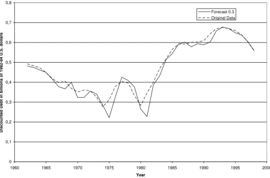
Hence, these …ndings suggest the existence of a band of sustainability, but also indicate that there are episodes in which the U.S. public debt moves out of the band. We use the quantile autoregressive model to make in-sample forecasts of the public debt for = 0:3 and 0:8:In other words, we want to estimate the upper and lower bounds of the sustainability band in order to identify the episodes during which public debt jumped out of the band. Figures 2 and 3 present the in-sample forecast for the 0:3th and 0:8th conditional quantile of the discounted public debt, respectively. Such trajectories provide a lower and upper bound for the band of sustainability. Note in these …gures that the original data data series of discounted public debt does not lie inside the band in about 16 years.
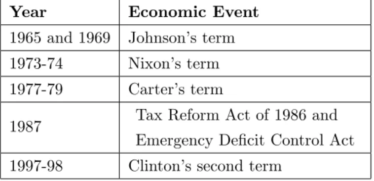
Table 7 reports the events associated to public debt levels larger than the upper bound. There are four important events: years following …rst and second oil shocks, recession beginning of Bush’s term, and Gulf war. This result shows that the occasional periods of expanding public debt in the U.S. are mostly motivated by unpredictable events like oil shocks and wars. Table 8 reports the events associated to public debt levels less than the lower bound. We notice that most of the periods during which U.S. debt moves beyond its lower bound are associated to episodes of persistent and strong …scal adjustment, as in Carter’s term, the Tax Reform Act of 1986 and Emergency De…cit Control Act, and the Clinton ’s second term. This suggests that the persistent decreasing in the US public debt observed during periods of …scal reforms stops when the public debt reaches a very low level deemed to be economically ine¢cient.
4.4 Global sustainability
for three di¤erent values of the block length, b;arbitrarily chosen. We considered 10,000 bootstrap replications
Note that the fundamental issue of the RBB bootstrap is its ability to simulate the weak dependence appearing in the original data series by separating the residuals in blocks. As the block length increases, the simulated dependence in the pseudo-series becomes more accurate (see appendix for details).
There is evidence that the discounted US federal debt is not a unit root process with signi…cance level of 5% for almost all values of b (except for b = 8, where we reject the unit root null at signi…cance level of 10%). Thus, the results in Table 9 suggest that the discounted U.S. federal debt is globally stationary.
We now test the null hypothesis that the discounted debt process has zero unconditional mean,
H0 : y = 0. Recall that testing such hypothesis correspond to testing the null 0 =E[ 0(Ut)] = 0. Notice that in our local analysis we tested the null 0( ) = 0 for various …xed quantiles. In
particular, results from Table 5 show that we cannot reject the null 0(0:5) = 0. Hence, under the
courageous assumption that the distribution of 0(Ut)is symmetric, not to reject 0(0:5) = 0would
be equivalent to not to reject 0 = 0. However, the distribution of 0(Ut) is probably skewed but,
even so, the results in Table 5 still provide some evidence that 0 = 0since we cannot reject the null
0( ) = 0for various quantiles around and including the median, that is, = 0:3;0:4;0:5;0:6;0:7.
Nevertheless, the distribution of 0(Ut)may be highly skewed and therefore we still need a formal test. We conduct a t-test for the unconditional meand and use the NBB resampling method with 10,000 replications to compute 5% critical values. Table 10 reports the t-statistic for the discounted public debt series. The reported results suggest that the unconditional mean of the autoregressive process is not statistically di¤erent from zero. This result associated with the QKS result for global stationarity present evidence that the public debt is globally sustainable.
5
Conclusion
In this work, we have empirically explored the question of whether the …scal policy in the United States is sustainable in the long-run using data on discounted public debt for the period from 1960 to 1998. The theoretical framework has been provided by the present value borrowing constrain that allows for a stochastic real interest rate as in Wilcox (1989) and Davig (2004). Following recent econometric studies that suggest the existence of regime shifts of …scal policy (Davig, 2004; Arestis et al. 2004), we use a quantile autoregression model recently proposed by Koenker and Xiao (2004a, 2004b) to test if the data provides evidence of asymmetries in the U.S. public debt.
Our econometric model accounts for many regime shifts and possesses robustness against dis-tribution misspeci…cation and outlier observations. We con…rm previous results in the literature concerning the existence of asymmetric dynamic in the U.S. public debt and global sustainability. As for local sustainability we report new results. In particular, three regimes of …scal policy were identi…ed: (1) when the public debt is low, …scal policy is unsustainable; (2) for values of the pub-lic debt around (and including) median, …scal popub-licy is sustainable characterizing what we called band of sustainability; (3) when public debt attains high values, …scal policy is unsustainable, even though the discounted public debt follow a stationary path.
List of Tables
Table 1: Results for the autoregressive order choice test excluding variableyt 3:
excluded variable
sup 2T Ln( ) estimate
5% critical value
10% critical value
H0:
3( ) = 0
yt 3 3.31 9.31 7.36 do not reject
Table 2: Results for the autoregressive order choice test excluding variableyt 2:
excluded variable
sup 2T Ln( ) estimate
5% critical value
10% critical value
H0:
2( ) = 0
yt 2 30.90 9.31 7.36 reject
Table 3: Results for the Symmetry test.
Coe¢cient test statistic 5% critical value OLS estimate j;OLS
H0:
j( ) = j;OLS
yt 1 4:190 2:140 1:56 reject
yt 2 3:123 2:140 0:63 reject
Table 4 : local stationarity results with t-statistics tn( ):
b1( ) tn( ) 2 H0 : 1( ) =
1
0.1 1.039 2.998 0.051 Do not reject at 5%
0.2 1.031 3.952 0.184 Do not reject at 5%
0.3 0.997 -0.252 0.107 Do not reject at 5%
0.4 0.961 -3.842 0.111 reject at 5%
0.5 0.950 -4.786 0.098 reject at 5%
0.6 0.943 -4.795 0.140 reject at 5%
0.7 0.879 -7.884 0.169 reject at 5%
0.8 0.863 -10.456 0.394 reject at 5%
Table 5: Results for intercept coe¢cient test.
b0( ) Ln( ) H0 :
b0( ) = 0 0.1 -43226.9 6.632 reject at
5%
0.2 -35994.42 5.061 reject at 5%
0.3 -12482.67 0.649 Do not re-ject at 5%
0.4 12548.71 0.282 Do not re-ject at 5%
0.5 20997.99 0.991 Do not re-ject at 5%
0.6 26649.5 1.912 Do not re-ject at 5%
0.7 67595.38 3.820 Do not re-ject at 5%
0.8 89075.46 10.163 reject at 5%
Table 6: Summary of results for local sustainability test.
Starionarity Zero
Un- condi-tional Mean
Sustainability
0.1 - -
-0.2 - -
-0.3 - Ok
-0.4 Ok Ok Ok
0.5 Ok Ok Ok
0.6 Ok Ok Ok
0.7 Ok Ok Ok
0.8 Ok -
-0.9 Ok -
-Table 7: years when the discounted public debt in larger than the 0.8th
conditional quantile forecast and associated political/economic event.
Year Economic Event
1975 right after …rst oil crisis 1981 and 1983 right after second oil crisis
1988 Recession beginning of Bush’s term 1991-92 Gulf War
Table 8: years when the discounted public debt in lower than the 0.3th
conditional quantile forecast and associated political/economic event.
Year Economic Event
1965 and 1969 Johnson’s term 1973-74 Nixon’s term 1977-79 Carter’s term
Table 9: Results for the global stationarity test.
Block length
b QKS
5% critical value
10%
critical value H0 : 1 = 1
8 6:3139 6:4807 5:6270 reject at 10%
12 6:3139 5:9743 5:1330 reject at 5%
16 6:3139 5:8237 5:1770 reject at 5%
Table 10: results for the unconditional mean test.
t 2:5%
critical value
97:5%
critical value H0 :intercept= 0
1;45 10 5 1;84 10 5 9;36 10 5 do not reject at5%
Table 11: Asymptotic critical values of the t-statistictn( )
2 1% 5% 10%
0.9 -3.39 -2.81 -2.50
0.8 -3.36 -2.75 -2.46
0.7 -3.30 -2.72 -2.41
0.6 -3.24 -2.64 -2.32
0.5 -3.19 -2.58 -2.25
0.4 -3.14 -2.51 -2.17
0.3 -3.06 -2.40 -2.06
0.2 -2.91 -2.28 -1.92
0.1 -2.78 -2.12 -1.75
6
Appendix I
6.1 Estimation of nuisance parameters
perfectly natural that the precision of quantile estimates should depend on this quantity, because it re‡ects the density of observations near the quantile of interest. If the data are very sparse at the quantile of interest, then it will be di¢cult to estimate. On the other hand, when the sparsity is low, so that observations are very dense, the quantile will be more precisely estimated." Thus, to estimate the precision of the th quantile regression estimate directly, the nuisance quantity
s( ) = f F 1( ) 1
must be estimated. To estimate s( )in the one-sample model we follow Siddiqui’s idea of di¤er-entiating the identity F F 1(t) = t: We …nd that the sparsity function is simply the derivative of the quantile function; that is
d dtF
1(t) =s(t):
So, just as di¤erentiating the distribution functionF yields the density functionf, di¤erentiating the quantile functionF 1yields the sparsity functions. Therefore, to estimates(t)we use a simple di¤erence quotient of the empirical quantile function; that is,
b
sn(t) =
b
Fn1(t+hn) Fbn1(t hn) 2hn
:
whereFbn1 is an estimate ofF 1andhnis a bandwidth that may tend to 0 asn! 1:A bandwidth rule proposed by Bo…nger (1975) is derived based on minimizing the mean squared error of the density estimator and is of ordern 15 :
hB =n
1 5
"
4:5s2(t) (s00(t))2
#1 5
:
In the absence of information about the form ofs( );we plug-in the Gaussian model to select bandwidth and obtain
hB=n
1 5
2 6 4 4:5
4 1(t)
2 ( 1(t))2+ 1 2
3 7 5 1 5 :
Koenker and Xiao (2004a) Monte Carlo results indicate that the Bo…nger bandwidth provides reasonable upper bound for bandwidth selection in testing parameter constancy. Thus, they suggest the utilization of a rescaled version of Bo…nger bandwidth (h= 0:6hB).
One way of estimating F 1(s) is to use a variant of the empirical quantile function for the linear model proposed in Bassett and Koenker (1982),
b
In summary,f F 1(t) can be estimated by
fn Fn1(t) = 1
b
sn(t)
= 1:2hB
xT (b( + 0:6hB) b( 0:6hB)):
For the long-run variance and covariance parameters, we may use the kernel estimators
2
! = M
X
h= M
k h
M C!!(h)
! ( ) = M
X
h= M
k h
M C! (h)
where ut =yt xTt ( ), (u) = I(u <0)and != yt:We choose to use the lag window
k h
M = 1
h
1 +M;
but what it is necessary is thatk( )is de…ned on[ 1;1]withk(0) = 1. The bandwidth (truncation) parameter M used was
M = integer 43
r
n
100 :
The quantities C!!(h) and C! (h) are simply the auto sample covariance of ! and sample covariance between ! and , respectively, i.e.:
C!!(h) = 1
n
X
!t!t+h
C! (h) = 1
n
X
!t bu(t+h)
.
6.2 The Non-overlapping Block Bootstrap (NBB) The NBB procedure can be summarized as follows:
Let by denote the sample mean of initial data series and suppose that l ln 2 [1; n] is an integer and b 1 is the largest integer satisfyinglb n:Then, de…ne the nonoverlapping blocks
ßi = y(i 1)l+1; :::; yil T
; i= 1; :::; b:
Step 2:Withm=kl, let m;ndenote the empirical estimate of the sample mean of the bootstrap sample y y1; :::; yl;:::;yf(b 1)l+1g; :::; ym obtained by writing the elements of ß 1; :::;ßk in a sequence, i. e.:
m;n = 1
m
m
X
j=1 yj:
Repeating steps 1-2 a great number of times (BB) we obtain a collection of pseudo-statistics
(1)
m;n; :::; m;n(BB): An empirical distribution based on the pseudo-statistics m;n(1); :::; m;n(BB) provide a consistent approximation of the distribution of by:Let Ct 2 and Ct 1 2 be the 1002 th and 100 1 2 th quantiles of the empirical distribution of m;n respectively, i.e.
P m;n Ct
2 = 2
and
P m;n Ct 1
2 = 1 2:
Then the null hypothesis will be rejected at the(1 ) level if
by Ct
2 or by Ct 1 2 : 6.3 Residual-Based Block Bootstrap for Unit Root Testing
This subsection describes the resampling method for detecting the presence of unit root in time series proposed by Paparoditis and Politis (2003).
For testing whether or not a series exhibit nonstationary behavior, the common assumption is that a time seriesfytgis either stationary around a (possibly nonzero) mean, or I(1), i.e., integrated of order one; as usual, the I(1) condition means that fytg is not stationary, but its …rst di¤erence series is stationary. The hypothesis test setup can then be stated as:
H0 : fytg is I(1) versus (14)
H1 : fytg is stationary.
in the literature where bootstrap approaches are applied to di¤erenced observations and/or the theory of bootstrap validity is often derived under the assumption that the observed process is unit root integrated. Furthermore, applying the block bootstrap to the di¤erenced series fails if the null hypothesis is wrong, i.e., the corresponding bootstrap statistic diverges to minus in…nity, leading to a loss of power. "
On carrying out the hypothesis testing (14) it is necessary to choose a parameter with the property that = 1 is equivalent to H0, whereas 6= 1 is equivalent to H1. Once decided which
parameter to use, Paparoditis and Politis (2003) suggests de…ning a new seriesfUtg as:
Ut= (yt yt 1)
fort= 1;2; :::where the constant is de…ned by =E(yt yt 1) so that E(Ut) = 0:This new
series is very useful because is stationaryalways: under H0 and/orH1:
In order to make clear how the RBB algorithm works, lets assume we want to carry out the traditional ADF. First, consider the ADF equation below
yt= yt 1+
p
X
j=1
j+1 yt j+ut (15) and let bn be the OLS estimator of . Next, de…ne the centered di¤erences
Dt=yt yt 1
1
n 1
n
X
s=2
(ys ys 1):
These di¤erences are the bootstrap analogous to the di¤erences of the original seriesfytgappearing in the ADF regression (15). We now describe the RBB bootstrap algorithm applied to the ADF case.
The RBBB testing algorithm to augmented Dickey-Fuller Type statistics
Step 1: …rst calculate the centered residuals
b
Ut= (yt enyt 1) 1
n 1
n
X
s=2
(ys enys 1); fort= 2;3; :::; n
where en is any consistent estimator of based on the observed datafy1; y2; :::; yng:
Step 2: Choose a positive integerb(< n), and leti0; i1; :::; ik 1 be drawn i.i.d with distribution
uniform on the set f1;2; :::; n bg; where k = h(nb1)i; and [ ] denotes the integer part of the number :The procedure constructs a bootstrap pseudo-seriesy1; :::; yl, wherel=kb+ 1;as follows:
yt =
(
y1
b+yt 1+Ubim+s
f or t= 1;
where
m = (t 2)
b
s = t mb 1
and b is a drift parameter that is either set equal to zero or is a pn-consistent estimator of :
Additionally, the procedure also generate a pseudo-series of l centered di¤erences denoted by
D1; D2; :::; Dl as follows: For the …rst block ofb+ 1observations we setD1 = 0 and
Dj =Di0+j 1 for j= 2;3; :::; b+ 1:
For the(m+ 1)th block,m= 1; ::; k 1 we de…ne
Dmb+1+j =Dim+j; wherej = 1;2; :::; b:
Step 3: We then calculate the regression of yt on yt 1 and on D1 1; Dt 2; :::; Dt p: Use the least squares estimator of the coe¢cient on yt 1 to compute the pseudo-statistic b :
Step 4: repeating steps 2-3 a great number of times (BB) we obtain a collection of pseudo-statistics b1; :::;bBB:An empirical distribution based on the pseudo-statistics b1; :::;bBB provide a consistent approximation of the distribution of bn under the null hypothesis H0 : = 1: The
-quantile of the bootstrap distribution in turn yields a consistent approximation to the -quantile of the true distribution (under H0), which is required in order to perform a -level test for H0.
The RBB testing algorithm to Kolmogorov-Smirnov test of global stationarity
To resample the limiting distribution of QKS given by (10), we follow steps 1 and 2 in the above procedure and replace steps 3 and 4 by
Step 3’: We then calculate the quantile regression of yt on yt 1 and on D1 1; Dt 2; :::; Dt p:
Use the quantile estimator of the coe¢cient onyt 1 to compute the pseudo-statistic b ( ):
Step 4’: repeating steps 2-3 a great number of times (BB) we obtain a collection of pseudo-statistics b1; :::;bBB:We then generate the pseudo-statistics
QKSi = sup
2T j
n(bi ( ) 1)j; f or i= 1; :::; BB:
An empirical distribution based on the pseudo-statistics QKS1; :::; QKSBB provide a consistent approximation of the distribution ofQKS under the null hypothesis H0: = 1:The -quantile of
the bootstrap distribution in turn yields a consistent approximation to the -quantile of the true distribution (underH0), which is required in order to perform a -level test for H0.
have low power, i.e., the experimental distribution does not represent the null hypothesis when the real data are generate by a stationary process.
The great advantage of the RBB process is that the algorithm manage to automatically (and nonparametrically) replicate the important weak dependence characteristics of the data, e.g., the dependence structure of the stationary process fytg and at the same time to mimic correctly the distribution of a particular test statistic under the null.
There is still the problem of how to choose the parameterbof block length. This parameter is of great importance to the Residual-based block bootstrap procedure to simulate weak dependence in the pseudo-series and thus providing power to the test. Observe in Step 2, that only one observation of each block is obtained as an aleatory drawn of the centered residual’s set with the others having centered residuals associated to the aleatory drawn.
The asymptotic results hold true for any block size satisfying
b! 1 but pb
n !0:
0 0,5 1 1,5 2 2,5
1955 1960 1965 1970 1975 1980 1985 1990 1995 2000 2005
Year
Billions of
1982-1984 Dollars
Undiscounted Debt
Discounted Debt
0 0,1 0,2 0,3 0,4 0,5 0,6 0,7 0,8
1960 1965 1970 1975 1980 1985 1990 1995 2000
Year
Disc
ounte
d Deb
t in billions of
198
2-8
4 U.S. dollar
s
Forecast 0.3 Original Data
Figure 2: Discounted public debt series and 0.3th conditional quantile in-sample forecast.
0 0,1 0,2 0,3 0,4 0,5 0,6 0,7 0,8
1960 1965 1970 1975 1980 1985 1990 1995 2000
Year
Discoun
ted Deb
t in Billio
ns of
1982-1984 dollars
Forecast 0.8 Original Data
7
Appendix II - Programs
############################################### ## Determines the optimal lag length
## Created by Raquel Sampaio ## last update June/30/2005
############################################### # Creating output …le
sink(”laglength.lis”, append=T)
# Reading data - must be in comma separated value format
y = read.csv(”serie7_x11.csv”, header=TRUE, sep=”;”, quote=”n””,dec=”.” , …ll=TRUE)
y = ts(y, start=1947, freq=1) # printing in…le name
print(”serie7_x11”) # uploading libraries library(stats)
library(quantreg) library(nlme)
# uploading external function source(”qdensity.txt”)
#____________________________________________________ # Imput Parameters
#____________________________________________________ # maximum lag to be analyzed
max.lag = 12 # selected quantiles
tau = seq(0.1, 0.9, by=1/200)
# parameter used in density function trim.prop = 0.025
#____________________________________________________ for (q in max.lag:1)
{
# this test uses level formulation instead of ADF formulation Y = y
for (i in 1:q) {
Y= ts.intersect(Y,lag(y,-i)) }
# Fitting model QAR
…t.QAR.1=rq(Y[,1] ~Y[,2:(q+1)],tau = -1) # estimating f(F^-1) - density function
# interpolating the density function for the selected quantiles (tau) h = rq.bandwidth(tau, nrow(Y))
h = 0.6 * h
trim = ((tau - h)<trim.prop)j((tau + h) >1 - trim.prop) qup = qrq1(…t.QAR.1, (tau + h)[!trim])
qlo = qrq1(…t.QAR.1, (tau - h)[!trim]) f.F.hat = (2 * h[!trim])/(qup - qlo) L=0
rho=0
for (quantil in 1:length(tau)) {
u= residuals(rq(Y[,1] ~Y[,2:(q+1)], tau = tau[quantil])) for (i in 1:length(u))
{
if (u[i] <0) rho[i]=u[i]*(tau[quantil]-1) else rho[i] = u[i]*tau[quantil]
}
V.hat = sum(rho)
# …tting QAR process without lag(q) variable, i.e., we excluded last column of Y u = residuals(rq(Y[,1] ~Y[,2:(q)], tau = tau[quantil]))
for (i in 1:length(u)) {
if (u[i]< 0) rho[i]=u[i]*(tau[quantil]-1) else rho[i] = u[i]*tau[quantil]
}
L[quantil]=(2*(V.til-V.hat)*f.F.hat[quantil])/(tau[quantil]*(1-tau[quantil])) }
sup.L = max(abs(L)) print(”q”)
############################################### ## Symmetry test
## Created by Z. Xiao
## Modi…ed by Raquel Sampaio ## last update June/30/2005
############################################### ”rq.bandwidth” <- function(p, n, hs = F, alph = 0.9){
#bandwidth selection for sparsity estimation two ‡avors: #Hall and Sheather(1988, JRSS(B)) rate = O(n^{-1/3}) #Bo…nger(1975, Aus. J. Stat) – rate = O(n^{-1/5})
PI<- 3.14159 X0<- qnorm(p)
f0<- (1/sqrt(2 * PI)) * exp(-(x0^2/2)) if(hs == T)
n^(-1/3) * qnorm(1 - alph/2)^(2/3) * ((1.5 * f0^2)/(2 * x0^2 + 1))^(1/3)
else n^-0.2 * ((4.5 * f0^4)/(2 * x0^2 + 1)^2)^0.2 }
”qrq1”<-function(s1, a) {
#computes linearized quantiles from rq data structure
#Note that the rq data structure here is new and has a third row with V in it. #s is the rq structure e.g. rqr(x,y)
#a is a vector of quantiles required r <- s1$sol[1, ]
q<- s1$sol[2, ] q<- c(q[1], q) J <- length(r)
r <- c(0, (r[1:J - 1] + r[2:J])/2, 1) u<- rep(0, length(a))
for(k in 1:length(a)) { i<- sum(r<a[k])
w<- (a[k] - r[i])/(r[i + 1] - r[i]) u[k]<- w * q[i + 1] + (1 - w) * q[i]
u }
”qdensity”<- function(z1,alpha,n) {
#Computes quantile density function estimate , fhat(F^{-1}(tau)) #Using trimming proportion alpha
#Sample Size n is required parameter #argument sol is the output of rq(x,y) #returns vector of quantile density estimates p<- z1$sol[1, ]
h<- rq.bandwidth(p, n, hs=F) h<- 0.6*h
trim<- ((p - h)<alpha) j((p + h)> 1 - alpha) qup<- qrq1(z1, (p + h)[!trim])
qlo <- qrq1(z1, (p - h)[!trim]) s <- (2 * h[!trim])/(qup - qlo) return(s,trim)
}
sink(”symmetry_level.lis”, append=T) library(quantreg)
alpha<- 0.05 # Reading data
y = read.csv(”disc_debt.csv”, header=TRUE, sep=”;”, quote=”n””,dec=”.”, …ll=TRUE) x = ts(y, start=1900, freq=1)
print(”disc_debt”) n<- length(x) p<- 2
# lag length = p
# Taking …rst di¤erence of series w = x - lag(x,-1)
# Generating ADF regressors with largest di¤erence lag equals p. Intercept not included Reg1 = lag(x,-1)
for (i in 2:p) {
}
# including intercept in regressor matrix
ones = ts(rep(1,(n-p+2)),start=start(Reg1), freq=1) Reg2 = ts.intersect(ones, Reg1)
# Reg1 = regressor without intercept in ADF regression # Reg2 = regressor with an intercept in ADF regression omega0<- t(Reg2)%*%Reg2
ome<- chol(omega0)
# Sets the coe¢cient to be tested
# if test.coef equals 1, coe¢cient of the …rst lag will be tested # if test.coef equals 2, coe¢cient of the …rst di¤erence will be tested for ( test.coef in 1: p)
{
ome22 <- ome[1+test.coef,1+test.coef]
# note this ome22 is not the same Omega22 in the paper. Y = ts.intersect(x, Reg1)
z <- rq(Y[,1] ~Y[,2:(p+1)], tau = -1) tao<- z$sol[1,]
btao = z$sol[4+test.coef,] L<- length(tao)
# OLS estimation, LAD could also be used here zols <- lm(Y[,1] ~Y[,2:(p+1)])
olse <- coef(zols)
bols<- olse[1+test.coef] den <- qdensity(z, alpha, n) score<-akj(z$sol[4,],z$sol[4,])
V <- ome22*den$s*(btao-bols*rep(1,L))[!den$trim] gdot<- cbind(rep(1,L)[!den$trim],-score$psi[!den$trim]) tao<- tao[!den$trim]
dtao<- di¤(c(0,tao)) dV <- c(0,di¤(V)) x1<- gdot*sqrt(dtao)
y1<- rev(dV/sqrt(dtao))
bhat<- lm.…t.recursive(x1,y1,int=F) bhat<- rbind(rev(bhat[1,]),rev(bhat[2,])) dH <- diag(gdot%*%bhat)*dtao
H <- cumsum(dH) kmin<- 0.1*n L<- length(tao) kmax<- L-kmin V <- V[kmin:kmax] H <- H[kmin:kmax] ks<- max(abs(V-H)) print(”test.coe¢cient”) print(test.coef)
############################################### ## Estimates the tn statistics used in local unit root tests
## Estimates the Ln statistics used in local unconditional mean test ## Created by Raquel Sampaio
## last update June/30/2005
############################################### # Uploading libraries
library(stats) library(quantreg) library(nlme)
# Uploading external functions source(”qdensity.txt”)
# Generating output …le #sink(”tnqunit.lis”)
# Reading in…le data - must be in comma separated value format
y = read.csv(”disc_debt.csv”, header=TRUE, sep=”;”, quote=”n””,dec=”.”, …ll=TRUE) y = ts(y, start=1947, freq=1)
print(”disc_debt”)
#____________________________________________________ # Input Parameters
#____________________________________________________ # Indicates if the local unconditional mean must be tested
# if lum=1, this condition must be tested lum=1
# frequency of data in a year freq = 1
# lag length in ADF formulation - should be determined with program ”laglength.txt” # Observe that laglength program determines length in level formulation
# you must use: q= (laglength result) - 1 q = 1
# maximum lag used in long run covariances estimations # truncation lag
# Selected quantiles
tau = seq(0.1, 0.9, by=0.05)
#____________________________________________________
Un.o = 0
alpha1.hat.o = 0 alpha0.hat.o = 0 f.F.hat = 0 tn = 0 I = 0 V.til = 0 V.hat = 0 Ln = 0 u = 0 phi = 0 ker = 0
#cov.w.phi = 0 sigma.w.phi = 0 delta2 = 0
# taking …rst di¤erence of series w = y - lag(y,-1)
# generating matrix W of di¤erences of original series W = w
if (q!=0) {
for (i in 1:q) {
W= ts.intersect(W,lag(w,-i)) }
}
# generating matrix Y with q lags in w Y = ts.intersect(y,lag(y,-1))
if (q!=0) {
{
Y= ts.intersect(Y,lag(w,-i)) }
}
# Fitting QAR model
…t.QAR.1=rq(Y[,1] ~Y[,2:(q+2)],tau = -1) # estimating f(F^-1) - density function
# interpoling the density function for the selected quantiles (tau) h = rq.bandwidth(tau, nrow(Y))
h = 0.6 * h
trim = ((tau - h)<trim.prop)j((tau + h) >1 - trim.prop) qup = qrq1(…t.QAR.1, (tau + h)[!trim])
qlo = qrq1(…t.QAR.1, (tau - h)[!trim]) f.F.hat = (2 * h[!trim])/(qup - qlo) # Generating projection matrix o = rep(1, times=nrow(Y))
X= ts(o, start=start(Y), freq=freq) if (q!=0)
{
for (i in 1:q) {
X= ts.intersect(X,lag(w,-i)) }
}
aux = solve(crossprod(X)) PX = X%*%aux%*%t(X)
aux = sqrt(t(Y[,2])%*%PX%*%Y[,2]) # Inicializing variables
u = matrix(nrow=nrow(Y), ncol=length(tau)) Phi = matrix(nrow=nrow(Y), ncol=length(tau)) alpha.hat.o = matrix(nrow=length(tau), ncol=(q+2))
# Fitting an regression quantile process
…t.QAR=rq(Y[,1] ~Y[,2:(q+2)], tau = tau[quantil]) # Obtaining u_t_tau necessary to delta^2
u[,quantil] = residuals(…t.QAR) logical= u[,quantil]< 0
Phi[,quantil] = tau[quantil] - logical #Local sustainability Test: intercepto = 0? if(lum==1)
{
#Obtaining Ln(tau) statistics
alpha0.hat.o[quantil] = coe¢cients(…t.QAR)[1] I = residuals(…t.QAR) <0
V.hat[quantil] = sum(residuals(…t.QAR) * (tau[quantil] - I)) …t.QAR.2=rq(Y[,1] ~Y[,2:(q+2)] - 1, tau = tau[quantil]) I = residuals(…t.QAR.2) <0
V.til[quantil] = sum(residuals(…t.QAR.2) * (tau[quantil] - I))
Ln[quantil] = 2*(V.til[quantil] - V.hat[quantil])*f.F.hat[quantil]/(tau[quantil]*(1-tau[quantil])) }
# Local satationarity test: alpha1 = 1? # Obtaining Un(tau) Statistics
Un.o[quantil] = nrow(Y) * (coe¢cients(…t.QAR)[2] - 1) alpha1.hat.o[quantil] = coe¢cients(…t.QAR)[2]
alpha.hat.o [quantil, ]= coe¢cients(…t.QAR) # Obtaining tn(tau) statistics
tn[quantil] = (f.F.hat[quantil]*aux*(alpha1.hat.o[quantil] - 1))/(sqrt(tau[quantil]*(1-tau[quantil]))) }
#____________________________________________________ # Obtaining delta^2 - nuisance parameter of tn limiting distribution
#____________________________________________________ phi = ts(Phi, start=start(Y), freq=freq)
for (j in 1:m) {
ker[j+1] = 2*(1 - (j/(1+m))) }
# obtating the long run var of w sigma2.w = sum(t(ker)%*%cov.w$acf)
# modifying kernel to only get the covariance of w with phi lags ker1 = rep(0, times=(1+2*m))
ker1[(m+1):(1+2*m)]<- ker
# obtaining the long run covariance of w with phi for (quantil in 1:length(tau))
{
aux = ts.intersect(w, phi[,quantil])
# obtaining the cross-covariance of w and phi lag max
cov.w.phi = ccf(aux[,2], aux[,1], type=c(”covariance”), lag.max=m) # obtaining the long run covariance of w and phi
sigma.w.phi[quantil] = sum(t(ker1)%*%cov.w.phi$acf) # obtaining delta^2
delta2[quantil] = (sigma.w.phi[quantil])^2/(sigma2.w * tau[quantil]*(1-tau[quantil])) }
#____________________________________________________ # Obtaining tn Critical values - uses delta^2 and Hansen’s table
#____________________________________________________ d2 = 0
tabela.5 = 0 tabela.10 = 0 tn.C.5 = 0 tn.C.10 = 0
tn.unit.root = as.character(length(tau))
if (lum==1) {Ln.unit.root = as.character(length(tau))} # uploads Hansen’s table
d2 = seq(0.9, 0.1, by=-0.1)
tn.C.5 = approx(d2, tabela.5, delta2, rule = 2) tn.C.10 = approx(d2, tabela.10, delta2, rule = 2) # Unity root local test result
for (quantil in 1:length(tau)) {
if (tn[quantil] < tn.C.5$y[quantil]) tn.unit.root[quantil] = ’rejeita’ else tn.unit.root[quantil] = ’nao rejeita’
}
# Unconditinal mean local test result if (lum==1)
{
for (quantil in 1:length(tau)) {
if(Ln[quantil]>3.84) Ln.unit.root[quantil] = ’rejeita’ else Ln.unit.root[quantil] = ’nao rejeita’ }
}
# Printing results cbind(trim.prop, q, m)
aux1 = cbind(tau, alpha.hat.o) print(aux1)
aux1 = cbind(tau,alpha1.hat.o, tn, tn.unit.root) print(aux1)
if (lum==1) {
aux1 = cbind(tau,alpha0.hat.o, Ln, Ln.unit.root) print(aux1)
############################################### ## Testing for global unit root with QKS.Un statistics
## Critical Values are obtained by resampling with RBBB ## Created by Raquel Sampaio
## last update July/08/2005
############################################### # Uploading libraries
library(stats) library(quantreg) library(nlme)
#Uploading density function source(”qdensity.txt”) # Creating output …le
#sink(”Br_RBBB_QKSresults.lis”, append=T) #sink(”RBBB_QKS.lis”)
sink(”RBBB_QKS.lis”, append=T) # Reading data in csv format
y = read.csv(”Br_serie7.csv”, header=TRUE, sep=”;”, quote=”n””,dec=”.”, …ll=TRUE) y = ts(y, start=1947, freq=1)
print (””) print (””) print (””) print (””) print (””)
date.system = Sys.time() print(date.system) print(”Br_serie7”)
#____________________________________________________ # Input Parameters
#____________________________________________________ # lag length in ADF formulation - should be determined with program ”laglength.txt” # Observe that laglength program determines length in level formulation
# you must use: q= (laglength result) - 1 q = 1
# if intercept.0 = 1, intercept must be considered # if intercept.0 = 0, model does not include intercept intercept.0 = 1
# frequency of data in a year freq = 1
# number of samples in bootstrap BB = 1000
# variable used in desity function estimation trim.prop = 0.025
# Selected quantiles - must be a large sample tau = seq(0.1, 0.9, by=1/200)
# selected blocks length
block.vector = c(14, 16, 18, 20, 22, 24)
#____________________________________________________ print(”q”)
print(q)
print(”intercepto.0”) print(intercept.0) print(”BB”) print(BB) Un.o = 0
alpha1.hat.o = 0 alpha0.hat.o = 0 f.F.hat = 0 tn.o = 0
# …rst di¤erence of series w = y - lag(y,-1)
# generating matrix Y with q lags in w Y = ts.intersect(y,lag(y,-1))
if (q!=0) {
for (i in 1:q) {
}
# Obtaining Un statistics for original data Un.o = matrix(nrow=length(tau), ncol=1)
alpha1.hat.o = matrix(nrow=length(tau), ncol=1) for (quantil in 1:length(tau))
{
# Fitting QAR model
…t.QAR=rq(Y[,1] ~Y[,2:(q+2)], tau = tau[quantil])
Un.o[quantil] = (length(y)-q) * (coe¢cients(…t.QAR)[2] - 1) alpha1.hat.o[quantil] = coe¢cients(…t.QAR)[2]
}
# Obtaining QKS statistics for original data QKS.Un.o = max(abs(Un.o), na.rm=T)
#____________________________________________________ # Bootstrap
#____________________________________________________ Un.star = matrix (nrow = length(tau), ncol = BB)
alpha1.star = matrix (nrow = length(tau), ncol = BB) QKS.Un.star = 0
QKS.Un.C95.star = 0 QKS.Un.C90.star = 0 # Fitting OLS model OLS # with intercept
if (intercept.0 == 1) {
OLS.…t = lm(Y[,1] ~Y[,2:(q+2)])
# obtaining …rst autoregressive coe¢cient beta.hat = coe¢cients(OLS.…t)[2]
# obtaining the intercept estimate mu.hat = coe¢cients(OLS.…t)[1] # obtaining residuals
# this may seen to be strange, but it is correct # residuals must not be the same as OLS …t residuals resid = y - beta.hat*lag(y,-1) - mu.hat
#without intercept if (intercept.0 == 0) {
OLS.…t = lm(Y[,1] ~Y[,2:(q+2)]-1)
# obtaining …rst autoregressive coe¢cient beta.hat = coe¢cients(OLS.…t)[2]
# obtaining residuals
# this may seen to be strange, but is correct
# residuals must not be the same as OLS …t residuals resid = y - beta.hat*lag(y,-1)
}
# generating centered residuals resid.center = resid - mean(resid) # generating centered di¤erence series d = w - mean(w)
n=nrow(Y)
for (i in 1:length(block.vector)) {
block = block.vector[i] for (b in 1:BB)
{
k = trunc((n-1)/block) l = k*block+1
# generating random values of standard uniform distribution i = runif(k)
# transforming random values from [0,1] range to [1,number of blocks] i = (n-block)*i
# transforming decimal values in integers that speci…es the blocks i = ceiling(i)
# generating y* pseudo-series y.star = ts(Y[1:l,1])
for (t in 2:l) {
y.star[t] = y.star[t-1]+resid.center[i[m+1]+s] }
# generating centered di¤erences pseudo-series d.star = ts(0*Y[1:l,1])
for(j in 2:(block+1)) {
d.star[j] = d[i[1]+j-1] }
for(m in 1:(k-1)) {
for (j in 1:block) {
d.star[m*block+1+j] = d[i[m+1]+j] }
}
# generating matrix of pseudo-series Y.star = ts.intersect(y.star, lag(y.star,-1)) if (q!=0)
{
for (i in 1:q) {
Y.star = ts.intersect(Y.star,lag(d.star,-i)) }
}
# Obtaining Un*(tau) statistics for bootstrap sample for (quantil in 1:length(tau))
{
…t.QAR=rq(Y.star[,1] ~Y.star[,2:(q+2)], tau = tau[quantil]) Un.star[quantil,b] = (l-q) * (coe¢cients(…t.QAR)[2] - 1) alpha1.star[quantil,b] = coe¢cients(…t.QAR)[2]
}
# obtaining QKS* statistics for bootstrap sample QKS.Un.star[b] = max(abs(Un.star[,b]), na.rm=T) }# End of bootstrap