FUNDAC¸ ˜AO GETULIO VARGAS ESCOLA DE ECONOMIA DE S ˜AO PAULO
JO ˜AO MARCOS BASTOS VILAR GARCIA
ASYMMETRIC PRICE ADJUSTMENT AND LOSS AVERSION
ASYMMETRIC PRICE ADJUSTMENT AND LOSS AVERSION
Dissertac¸˜ao apresentada `a Escola de Economia de S˜ao Paulo da Fundac¸˜ao Getulio Vargas como requisito para obtenc¸˜ao do t´ıtulo de Mestre em Economia de Empresas
Campo de Conhecimento: Economia Comportamental
Orientador: Prof. Dr. Bruno Ferman
Bastos Vilar Garcia, João Marcos.
Asymmetric price adjustment and loss aversion / João Marcos Bastos Vilar Garcia. - 2016.
26 f.
Orientador: Bruno Ferman
Dissertação (mestrado) - Escola de Economia de São Paulo.
1. Gasolina – Mercado - Brasil. 2. Gasolina – Preços - Brasil. 3. Controle de preços. 4. Gasolina – Oferta e procura. 5. Equilíbrio econômico. I. Ferman, Bruno. II. Dissertação (mestrado) - Escola de Economia de São Paulo. III. Título.
Dissertac¸˜ao apresentada `a Escola de Economia de S˜ao Paulo da Fundac¸˜ao Getulio Vargas como requisito para obtenc¸˜ao do t´ıtulo de Mestre em Economia de Empresas
Campo de Conhecimento: Economia Comportamental Data de aprovac¸˜ao
/ /
Banca Examinadora:
Prof. Dr. Bruno Ferman (Orientador) FGV-EESP
Prof. Dr. Bernardo Guimar˜aes FGV-EESP
Prof. Dr. Paulo Furquim Insper
ABSTRACT
Asymmetric price adjustment is observed in several markets, most notably gasoline retail: a cost increase is passed through to consumers faster than a cost decrease. I develop a consumer-search model that generates this prediction under loss aversion. A fraction of consumers are ignorant of market prices and can choose to acquire information costly, allowing firms to profit with price dispersion. Asymmetric price adjustment emerges if consumers are loss-averse in relation to a reference price. Higher costs make consumers more willing to search, but also lower the probability of finding low prices, generating convexity in the cost-price relation.
frac¸˜ao dos consumidores ignora os prec¸os no mercado e pode adquirir informac¸˜ao a um custo, o que permite que as firmas tenham lucro com dispers˜ao de prec¸os. Ajuste assim´etrico de prec¸o emerge se os consumidores s˜ao aversos a perdas em relac¸˜ao a um prec¸o de referˆencia. Custos mais altos tornam os consumidores mais dispostos a procurar, mas tamb´em diminui as chances de encontrar prec¸os baixos, gerando uma relac¸˜ao custo-prec¸o convexa.
Contents
1 Introduction 6
2 Baseline Model 8
3 Reference-Price Model 13
4 Conclusion 19
A Intermediate equilibrium 22
A.1 Existence . . . 22 A.2 Unicity . . . 24 A.3 Proof of Theorem 3 . . . 25
1 Introduction
Output prices take longer to adjust when input prices fall than when they rise. The empirical literature documenting this fact, often called rockets and feathers, is large and mostly focused on specific markets, specially the gasoline retail market 1. In particular, Peltzman (2000) finds
evidence of this asymmetry in around two thirds of 200 analysed markets, suggesting it might be an important feature in the economy. More precisely, symmetric price adjustment means that, first, contemporaneous response is larger after positive shocks than after negative shocks. Second, the effects of negative shocks take longer to be fully incorporated into prices. Finally, after several periods, there is no difference in cumulative response i.e., passthrough is the same on the long run. Despite the empirical evidence, research on theoretical explanations for this phenomenon has been scarcer.
In this paper I develop a consumer-search model, similar to Varian (1980), Burdett and Judd (1983), and Benabou and Gertner (1993), where the introduction of loss aversion relative to a backward-looking reference price gives rise to asymmetric pricing. A fraction of consumers are ignorant of market prices but can learn them at a cost. Firms are able to profit from this ignorance generating price dispersion, but the ability to search limits how much can be extracted. Relaxing the assumption of traditional outcome-based utility, consumers also derive utility from losses-gains in relation to a backward-looking reference. Consumers become less inclined to search after a fall in costs, as prices are low relative to their reference (and vice versa). Asymmetry in adjustment is caused by two mechanisms. First, a cost increase raises the whole price distribution, reducing the chance to find a low price, thus having a second order positive effect on willingness to search, generating convexity in the cost-price relation. Second, for sufficiently large shocks, the marginal passthrough is complete, but this happens for relatively small positive shocks and only large nega-tive shocks.
Asymmetry in price responses is not a feature either of classical models of perfect or imperfect competition. Some initial explanations proposed were based on inventory adjustment costs Boren-stein et al. (1997) or collusion Karrenbrock (1991). However, Peltzman (2000) finds no association ofrockets and featherswith inventories or menu costs, nor with measures of market concentration.2
1Examples in gasoline retail include Karrenbrock (1991); Borenstein et al. (1997); Johnson (2002); Verlinda (2008);
Deltas (2008), among others. Other specific markets in which this phenomenon is documented are banking Hannan and Berger (1991); Neumark and Sharpe (1992); Arbatskaya and Baye (2004), and agrarian products Boyd and Brorsen (1988); Goodwin and Holt (1999); Ward (1982)
2
7
Other models that generate rockets and feathers using a consumer-search model are Tappata (2009), Yang and Ye (2008) and Lewis (2011). Tappata (2009) uses a search model where con-sumers observe only the past realizations of costs and choose search intensity. When the marginal cost is expected to be higher, firms will choose less disperse prices, meaning gains from search are low (and vice versa). Under persistent cost realizations, differential search efforts creates asym-metry in initial responses to shocks, though total adjustment time is symmetrical. Similarly, in the Yang and Ye (2008) model, consumers are only informed of past realizations when they choose to search. Asymmetry in adjustment is generated by asymmetric learning: because more consumers search after a cost increase, adjustment is fast. The main differences in this paper are that I make no assumptions on the process generating marginal cost realizations, and costs are common knowledge at all times.
Closer to this paper is Lewis (2011), that proposes a consumer-search model, in which con-sumers have adaptive expectations over the market distribution of prices. Following positive cost shocks, consumers do not update their belief of price distribution, so a larger share of consumers will search, making the market more competitive in the short run (and vice-versa). The asymme-try comes from concavity in the relation cost-prices. In contrast, in the model presented in this paper, consumers have fully rational expectations and the dynamic effect on demand comes via non-standard preferences depending on past realizations.
2 Baseline Model
Consider a market with two firms selling a homogeneous good, with the same marginal cost
cand no fixed costs. At the beginning of the period, firms observe the realized marginal cost and compete in prices. Assume firms are myopic, so there is no motive for collusion: they simply maximize current profit. There are two types of consumers: informed consumers, who exist in measures, observe both posted prices; while uninformed consumers, in measure 1−s, observe the marginal cost, but not realized prices. Uninformed consumers initially observe only the price posted by one of the firms, at random. They may, then, pay a search cost, k, to learn the other firm’s price. A consumer that searches always buys for the lowest price at no additional cost. Each consumer has unit demand up to priceν1. Informed consumers simply buy one unit of the good for
the lowest price in the market. A consumer that chooses to buy at pricepderives utility:
u(p) =ν−p
Consumers rationally form a prior over the price distribution,L(p)after observing the cost re-alization and choose a search strategy informed by this prior. Firms choose their pricing strategies and consumers choose their search strategies simultaneously. Since costs are observed and firms choose their strategies independently, there is no need to update consumers’ priors after observing the first price. Therefore, search strategy takes the form of a cut-off price, beyond which consumers will choose to search. A market equilibrium is a description of each players strategies where con-sumers search optimally and firms’ pricing strategies are best responses, given a realization of the marginal cost and other players’ strategies.
Theorem 1 There is no pure-strategy equilibrium. Varian (1980)
Suppose there is a pure-strategy equilibrium with firms playingp∗
1 andp
∗
2. First, supposep
∗
1 =
p∗
2 > c. Then, it is a profitable deviation for firm 1 to lower its price slightly, taking the demand
from all searchers while losing very little margin. Now, suppose p∗
1 = p
∗
2 = c. Then, firm 1 can
increase it’s price, forgo informed-consumer demand and still obtain a profit selling to uninformed consumers: for a small enough increase, consumers will not pay the search cost, even if they believe
9
they can get a lower price. Finally, supposec ≤ p∗
1 < p
∗
2. If firm 1 increases its price marginally,
its total demand will not be affected: the number of consumers that search may increase, but all searching consumers will buy from firm 1 if its price is still lower than firm 2. Therefore, firm 1 can increase its margin without losing any demand. Hence, there can be no equilibrium in pure strate-gies. Thebusiness-stealingmotive pushes to always undercut the competition, while the surplus-appropriationmotive leads to acting as a monopolist over the non-searchers. This trade-off creates price dispersion in equilibrium i.e., firms will play mixed strategies. Therefore, I look for symmetric mixed-strategies equilibria.
An uninformed consumer, having observed pricep1will choose to search if the expected value of doing so outweighs the cost of searching. Given a prior belief over the other firm’s price, repre-sented by the cumulative distribution functionL(p2), the consumer will search if:
k ≤
Z p1
−∞
(u(p2)−u(p1))l(p2)dp2 = Z p1
−∞
(p1 −p2)l(p2)dp2 (1)
Callp˜the price that makes the consumer indifferent between buying and searching.
Theorem 2 There is a mixed-strategy equilibrium where both firms randomize prices in the inter-val[p(c, k, s);p(c, k, s)], following density functionf(p), with:
p=c+ 2sk 1 +s
1 +s
1−s −log
1 +s
1−s
−1
−1
p=c+ 2sk 1−s
1 +s
1−s −log
1 +s
1−s
−1
−1
f(p) = (p−c)−2
k
1 +s
1−s −log
1 +s
1−s
−1
−1
Π(p) = (p1−c)
(1−s) 2 +s
Z p
p1
f(p2)dp2
(2)
For any mixed strategy to be optimal, profits must be the same at all prices on support, in particular, at the lowest price, where the firm is assured to sell to all informed consumers, and at the highest price, only to the uninformed. This condition gives:
Π(p) = (p−c)(1−s)
2 = (p−c)
(1 +s)
2 (3)
At all prices on support, the firm must be indifferent between charging this price or a marginally higher price. Differentiating equation 2 in respect top1, equating to zero and rearranging wields:
(1−s) 2 +s
Z p
p1
f(p2)dp2 = (p1−c)sf(p1) (4)
Figure 1 illustrates this trade-off. A marginal price increase has two effects on profits. First, there is an increase in mark-up, raising expected profits proportionally to current expected demand, the shaded area in the figure plus the demand from uninformed consumers. Second, there is a lower chance that the firm has the lowest price on the market and is able to sell to informed consumers, decreasing expected demand, proportionally to f(p1) in the figure. Equation 4 requires that the
optimal strategy makes these two effects equal at all prices on support. Differentiating a second time and rearranging gives:
2f(p1) + (p1−c)f
′
(p1) = 0
Solving this differential equation, we get:
f(p1) =
a
(p1−c)2
(5)
11
Figure 1: At pricex, expected demand equals(1−s)plus the shaded area
Plugging equation 5 in equation 4 and rearranging gives:
p−c= 2sa
1−s (6)
Then, using equation 3, we get:
p−c= 2sa
1 +s (7)
Using these equations we can easily compute the mean price, still as a function ofa:
E[p] =a
Z p
p
p
(p−c)2dp=c+alog
1 +s
1−s
(8)
Equations 5, 6 and 7 partially characterize the equilibrium as a function of variablea. Note that, whileadoes not have a clear economic interpretation, it parametrizes the equilibrium in a useful way and we can think of it as a measure of the market competitiveness. Average, minimum and maximum mark-ups are linear and increasing ona, as is price dispersion (measured asp−p).
p
k =a
Z p
p
p−p2
(p1−c)2
dp2
a=k
1 +s
1−s −log
1 +s
1−s
−1
−1
(9)
Now, equation 9 allows to fully characterize the equilibrium.
p=c+ 2sk 1−s
1 +s
1−s −log
1 +s
1−s
−1
−1
(10)
p=c+ 2sk 1 +s
1 +s
1−s −log
1 +s
1−s
−1
−1
(11)
E[p] =c+klog
1 +s
1−s
1 +s
1−s −log
1 +s
1−s
−1
−1
(12)
This model generates very simple predictions. In equilibrium firms charge marginal cost plus a random markup independent of cost realizations, meaning expected profits are constant and all cost shocks are fully passed on to consumers. There is a constant distribution of prices, where firms’ relative pricing position is randomized at each period.
13
3 Reference-Price Model
The key feature I introduce into the model is loss aversion. As proposed by Kahneman and Tversky (1979), loss aversion is one component of prospect theory, an alternative to the expected-utility theory of choice under risk. In prospect theory, lotteries are evaluated not for the value of each outcome, but for the change in value relative to some reference. Loss aversion means that losses relative to this reference are given greater importance than gains. The reference is typically assumed to be the status-quo or based on past experience. This type of utility function can explain some empirical anomalies in contexts of choice under risk. In the context of laboratory experiments, agents’ choice between two simple lotteries were strongly affected depending of whether the out-comes were framed as losses or gains, illustrating reference-dependence. Also, it helps explain why people generally refuse low-stakes lotteries with positive expected payoff Rabin (2000)1. Besides
choice under risk, reference-dependent utility seems to explain some anomalies in labor markets, namely that cab drivers and bicycle messengers seem to reduce labor supply or effort when wages are higher, consistent with working until a certain reference goal is reached Camerer et al. (1997); Farber (2005); Fehr and Goethe (2007).
Although both firms and consumers are making decisions under risk, I argue that it is reason-able that only consumers have reference-dependent preferences. Because each consumer pays a relatively small share of his or hers income in a given good this might be a ”good enough” heuristic rule. Retailers, on the other hand, might have their entire profits dependent on their pricing decision, giving strong incentives to find optimal decisions.
For simplicity, I will assume the reference to be the average price during the last period. Results would be qualitatively unchanged if the reference is a weighted average of past realizations. I specify the utility function as:
v(p, pr) = u(p) +m(p−pr) = ν−p−b(p−pr)✶{p−pr>0}
where b measures the intensity of loss aversion. Note that there is disutility associated with losses but no utility from gains relative to the reference. As long as the consumer is marginally more sensitive to losses, adding a positive utility to gains is equivalent to a reparametrization of the
1Agents with continuous and smooth utility functions are approximately risk-neutral with respect to lotteries with
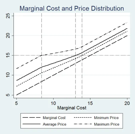
Figure 2: Prices after different realizations of the marginal cost (pr= 15,b= 1s=.5,k= 3)
model. In the stage game,pr is exogenous, but we will give it a dynamic interpretation making it equal to last period’s average price.
In this model, firms are myopic. They do not take into account that their pricing decision influ-ences consumers referinflu-ences in the future and, therefore, their demand. This hypothesis, although very restrictive, is necessary for my results.
Now, the no-search condition becomes:
k =
Z p
−∞
(v(p2, pr)−v(p, pr))f(p2)dp2 (13)
15
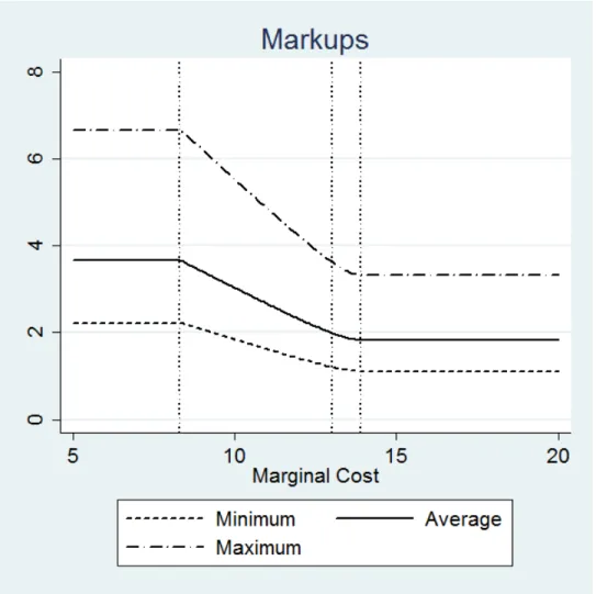
Figure 3: Markups after different realizations of the marginal cost (pr= 15,b= 1s=.5,k= 3)
different properties, as shown in figures 2 and 3. The general shape of the graph does not change with different parameters and there are no regions of indeterminacy or multiplicity.
In the first case, corresponding to the area left of the first vertical line in the figure, after a sufficiently strong fall in costs, competition forces prices down enough that all prices on support are lower than the reference price. This is the case if:
c≤pr−
2ks
1−s
1 +s
1−s −log
1 +s
1−s
−1
−1
=:c(pr, k, s, b) (14)
Then the equilibrium is identical to the baseline model, and characterized by equation 9. Since all prices are below the reference, no consumer is in the loss region, and search choices are un-changed.
c≥pr−
2ks
(1 +s)(1 +b)
1 +s
1−s −log
1 +s
1−s
−1
−1
=:c(pr, k, s, b) (15)
The equilibrium is characterized by:
a= k 1 +b
1 +s
1−s −log
1 +s
1−s
−1
−1
(16)
In this case, loss aversion has an effect identical to a reduction in the search cost, reducing the whole distribution of mark-ups. The qualitative characteristics of the equilibrium, however, are the same. In this region, marginal changes in cost are fully passed on to consumers.2
Finally, for realizations ofcbetween cand c, there are prices both higher and lower than the reference price on the support. The equilibrium is characterized by:
k=a
(1 +b)(1 +s) 1−s −log
1 +s
1−s
−blog
2sa
(1−s)(pr−c)
−1
− b(pr−c)(1 +s)
2s (17)
Which can be numerically solved for values ofk,s,b,candpr. I discuss existence and unicity of this condition in Appendix A.
In the baseline model and in the previous cases, a marginal change in cost has the effect of rising all prices by exactly the same amount. In this case, however, a marginal increase inc, ceteris paribus, has a different effect. Consider the consumer that faces the highest price on support. After a marginal increase in cost, if firms maintain the same mark-ups, both options the consumer has (searching or not) become less attractive, but loss aversion makes not searching marginally worse, as it is possible to find prices lower than the reference. This marginal consumer becomes more willing to pay the search cost, making the market more competitive. Thus, after a cost increase, prices will rise but mark-ups will go down, as will price dispersion (and vice versa, for a cost decrease).
Proposition 1 In the intermediate region, prices are convex inc.
17
I do not provide analytical proof of this proposition. It is, however, supported by simulation exercises described in Appendix B.
The convexity in the relationship between costs and price causes asymmetric adjustment i.e., price will rise more after a cost increase than it will fall after a cost decrease. Consider a marginal increase in cost. Utility from paying the highest price decreases faster than expected utility from searching. However, as all prices increase, there is a smaller chance of finding a price lower than the reference. Therefore, the utility from searching falls faster the higher prices are. This makes the markups fall with higher cost, but the fall is slower at higher prices.
Finally, callc∗
the cost that makesE[p] = pr. Note in figures 2 and 4 thatc
∗
is much closer to
cthen it is toc. This is an important general feature of the model.
Theorem 3
|c∗
−c|<|c∗
−c|
Proof in Appendix A.3.
This characteristic means that the largest possible effect of a positive cost shock on markups in any given period is bounded at a much smaller absolute value than that of a negative impact. See that, in figure 3, starting atc∗
, a cost increase, no matter how large can only compress the average markup to a little under 2, just barely under what it would be if cost did not change. A large cost decrease, however, can increase markups much more dramatically in one period.
Figure 4: Simulation of positive and negative cost shocks on price and markup distribution. (c = 13,∆c = 3,b = 1
19
4 Conclusion
Bibliography
Arbatskaya, M. and Baye, M. R. (2004). Are prices ’sticky’ online? Market structure effects and asymmetric responses to cost shocks in online mortgage markets. International Journal of In-dustrial Organization, 22(10):1443–1462,.
Benabou, R. and Gertner, R. (1993). Search with learning from prices: does increased inflationary uncertainty lead to higher markups? The Review of Economic Studies, 60(1):69–93.
Borenstein, S., Cameron, A. C., and Gilbert, R. (1997). Do gasoline prices respond asymmetrically to crude oil price changes. The Quarterly Journal of Economics, 112(1):305–339.
Boyd, M. S. and Brorsen, B. W. (1988). Price asymmetry in the U.S. pork marketing channel.
North Central Journal of Agricultural Economics, 10(1):103–109.
Burdett, K. and Judd, K. L. (1983). Equilibrium price dispersion. Econometrica, 51(4):955–969. Camerer, C., Babcock, L., Lowestein, G., and Thaler, R. (1997). Labor supply of New York City
cab drivers: one day at a time. Quarterly Journal of Economics, 112(2):407–441.
Chandra, A. and Tappata, M. (2011). Consumer search and dynamic price dispersion: an applica-tion to gasoline markets. The RAND Journal of Economics, 42(4):681–704.
Deltas, G. (2008). Retail Gasoline Price Dynamics and Local Market Power. The Journal of Industrial Economics, 56(3):613–628.
Farber, H. (2005). Is tomorrow another day? The labor supply of New York City cab drivers.
Journal of Political Economy, 113(1):46–82.
Fehr, E. and Goethe, L. (2007). Do workers work more if wages are high? Evidence from a ran-domized field experiment. The American Economic Review, 97(1):298–317.
Goodwin, B. K. and Holt, M. T. (1999). Price transmission and asymmetric adjustment in the U.S. beef sector. American Journal of Agricultural Economics, 81(3):630–637.
Hannan, T. H. and Berger, A. N. (1991). The rigidity of prices: evidence from the banking industry.
The American Economic Review, 81(4):938–945.
Hosken, D. S., McMillan, R. S., and Taylor, C. T. (2008). Retail gasoline pricing: What do we know? International Journal of Industrial Organization, 26(6):1425–1436.
Johnson, R. N. (2002). Search costs, lags and prices at the pump.Review of Industrial Organization, 20(1):33–50.
21
Karrenbrock, J. D. (1991). The behavior of retail gasoline prices: symmetric or not? Federal Reserve Bank of St. Louis Review, 73(4):19–29.
Lewis, M. S. (2011). Asymmetric price adjustment and consumer search: an examination of the retail gasoline market. Journal of Economics and Management Strategy, 20(2):409–449.
Neumark, D. and Sharpe, S. A. (1992). Market structure and the nature of price rigidity: evidence from the market for consumer deposits. The Quarterly Journal of Economics, 107(2):657–680. Peltzman, S. (2000). Prices rise faster than they fall.The Journal of Political Economy, 108(3):466–
502.
Rabin, M. (2000). Risk aversion and expected-utility theory: a calibration theorem. Econometrica, 68(5):1281–1292.
Tappata, M. (2009). Rockets and feathers: understanding asymmetric pricing. The RAND Journal of Economics, 40(4):673–687.
Varian, H. R. (1980). A model of sales. The American Economic Review, 70(4):651–659.
Verlinda, J. A. (2008). Do rockets rise faster and feathers fall slower in an atmosphere of local market power? Evidence from the retail gasoline market. The Journal of Industrial Economics, 56(3):581–612.
Ward, R. W. (1982). Asymmetry in retail, wholesale, and shipping point pricing for fresh vegeta-bles. American Journal of Agricultural Economics, 64(2):205–212.
Yang, H. and Ye, L. (2008). Search with learning: understanding asymmetric price adjustments.
A Intermediate equilibrium
A.1
Existence
We can write the equilibrium condition when the reference price is between the maximum and minimum prices as:
k+ b(pr−c)(1 +s)
2s =a
(1 +b)(1 +s) 1−s −log
1 +s
1−s
−1
−ablog
2sa
(1−s)(pr−c)
:=F(a) (18)
The right-hand size of this equation is increasing inafroma = 0until a maximum, and then is strictly decreasing. An equilibrium will exist if, and only if, this maximum is above the expression in the left-hand side.
Differentiating the right-hand side and equating to zero obtains:
F′
(a) = (1 +b)
1 +s
1−s −log
1 +s
1−s
−1
−blog
2sa
(1 +s)(pr−c)
= 0
log(a) = 1 +b
b
1 +s
1−s −log
1 +s
1−s
−1
+ log
(1 +s)(pr−c)
2s
ComputingF(a)at the equilibrium, first substituting onlylog(a):
a
(1 +b)(1 +s) 1−s −log
1 +s
1−s
−1
−a(1 +b)
1 +s
1−s −log
1 +s
1−s
−1
−ablog
(1 +s)(pr−c)
2s
−ablog
2s
(1 +s)(pr−c)
=ab
23
bexp
1 +b b
1 +s
1−s −log
1 +s
1−s
−1
+ log
(1 +s)(pr−c)
2s
≥k+ b(pr−c)(1 +s) 2s
b(pr−c)(1 +s) 2s
exp
1 +b b
1 +s
1−s −log
1 +s
1−s
−1 −1 ≥k
However, we are interested in this equilibrium only in the relevant region, the interval [c;c]. Therefore, compute this condition onˆc=λc+ (1−λ)c.
ˆ
c=pr−2ks
λ
1−s +
1−λ
(1 +b)(1 +s)
1 +s
1−s −log
1 +s
1−s
−1
−1
Substituting in the above condition:
b
1 +s
1−s −log
1 +s
1−s
−1
−1
λ(1 +s) 1−s +
1−λ
1 +b
e1+
b b (
1+s
1−s−log(
1+s
1−s)−1)−1 ≥1
λ1 +s
1−sb
1 +s
1−s −log
1 +s
1−s
−1 −1 e1+ b b ( 1+s
1−s−log(
1+s
1−s)−1)
+ (1−λ) b 1 +b
1 +s
1−s −log
1 +s
1−s
−1 −1 e1+ b b ( 1+s
1−s−log(
1+s
1−s)−1) ≥e
Calling 1+bb 1+1−ss−log
1+s
1−s
−1
=x,x >0the second term becomes:
ex x ≥e
It is easy to see that exx reaches a minimum ofeover the positive real numbers atx= 1. Similarly, callb−1 1+s
1−s−log
1+s
1−s
−1
=y,y >0the first term becomes:
ey y
1 +s
1−se
1+b ≥e
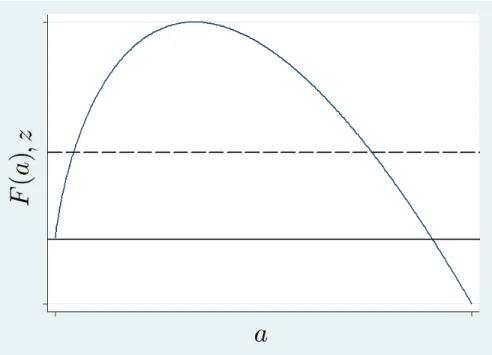
Figure 5: Equilibrium condition for the intermediate equilibrium: the curveF(a)equalsz, the dashed line
A.2
Unicity
In general, the condition for the intermediate equilibrium has two solutions. This is illustrated in figure 5. Callz the left-hand side of equation 18. FunctionF(a)equalsz either zero, one or two times. However, the crossing-from-above solution does not respect the conditionpr∈[p;p], and is not an equilibrium.
The intuition for this duality is the following: suppose the reference price is in the strategy sup-port and varya, shifting the whole price distribution. Remember this is the indifference condition between paying and searching for the consumer that faces the highest price. At low prices, the search cost is relatively high and dispersion is low, so it is better to buy. Asa rises the utility of buying falls faster than that of searching, due to loss aversion, until indifference is reached. Asa
25
A.3
Proof of Theorem 3
Letd(pr, k, s, b) =c
∗
−c+2c, such that, ifd(pr, k, s, b)>0, thenc
∗
is closer tocthan toc. Using equations 10, 11 and 12:
d(pr, k, s, b) = k
1 +s
1−s −log
1 +s
1−s
−1
−1
s
1−s + s
1 +s −log
1 +s
1−s
d(pr, k, s, b)∝
2s
1−s2 −log
1 +s
1−s
Note that this function is continuously differentiable if s ∈ [0; 1], has a root ins = 0 and its derivative with respect tosis:
4s2
(1−s2)2 >0
B Convexity Analysis Simulations
This section briefly describes the simulations that support proposition 1. The first step is creating arrays of parameterss,bandk. I use:
• s ∈[0.5; 0.99]1
• b ∈[0; 5]
• k ∈[1; 5]
I fixpr = 10, without loss of generality, because equation 17 depends only on the differencepr−c, and we will findcendogenously.
Next, compute c(pr, s, b, k)and c(pr, s, b, k) for each parameter triad using equations 14 and 15. For each parameter triad, generate an array of values betweencand cand numerically solve equation 17 for each value of the cost realization, choosing initial conditions carefully to avoid the excluded equilibrium. This gives functiona(pr, s, b, k, c). If the function is convex, the difference between the value of a at any pair of consecutive points in a cost array must be lesser than the difference for the preceding pair. Formally, for any three valuesc1 < c2 < c3:
[a(pr, s, b, k, c3)−a(pr, s, b, k, c2)]−[a(pr, s, b, k, c2)−a(pr, s, b, k, c1)]≥0
Therefore, I compute this difference at every successive pair in each array. Results indicate that the inequality always holds in the analysed region, corroborating the proposition.
1